Enhanced computation method of topological smoothing on shared memory parallel machines

(1)

R E S E A R C H

Open Access

Enhanced computation method of topological

smoothing on shared memory parallel machines

Ramzi Mahmoudi

*

and Mohamed Akil

Abstract

To prepare images for better segmentation, we need preprocessing applications, such as smoothing, to reduce noise. In this paper, we present an enhanced computation method for smoothing 2D object in binary case. Unlike existing approaches, proposed method provides a parallel computation and better memory management, while preserving the topology (number of connected components) of the original image by using homotopic transformations defined in the framework of digital topology. We introduce an adapted parallelization strategy called split, distribute and merge (SDM) strategy which allows efficient parallelization of a large class of topological operators. To achieve a good speedup and better memory allocation, we cared about task scheduling and managing. Distributed work during smoothing process is done by a variable number of threads. Tests on 2D grayscale image (512*512), using shared memory parallel machine (SMPM) with 8 CPU cores (2× Xeon E5405 running at frequency of 2 GHz), showed an enhancement of 5.2 with cache success rate of 70%.

1. Introduction

Smoothing filter is the method of choice for image prepro-cessing and pattern recognition. For example, the analysis or recognition of a shape is often perturbed by noise, thus the smoothing of object boundaries is a necessary prepro-cessing step. Also, when warping binary digital images, we obtain a crenellated result that must be smoothed for bet-ter visualization. The smoothing procedure can also be used to extract some shape characteristics: by making the difference between the original and the smoothed object, salient or carved parts can be detected and measured.

Smoothing shape has been extensively studied and many approaches have been proposed. The most popular one is the linear filtering by Laplacien smoothing for 2D-vector [1] and 3D mesh [2]. Other approach by morphological filtering can be applied directly to the shape [3] or to cur-vature plot of the object’s contour [4]. Unfortunately none of these operators preserve the topology (number of con-nected components) of the original image. In 2004, our team introduced a new method for smoothing 2D and 3D objects in binary images while preserving topology [5]. Objects are defined as sets of grid points, and topology preservation is ensured by the exclusive use of homotopic transformations defined in the framework of digital

topology [6]. Smoothness is obtained by the use of morphological openings and closings by metric discs or balls of increasing radius, in the manner of alternating sequential filters [7]. The authors’efforts have brought about two major issues such as preserving the topology and the multitude of objects in the scene to smooth out without worrying about memory management, latency or cadency of their filter. This paper describes an enhanced computation method of topological smoothing filter that assure better performance. We present also a new paralle-lization strategy, called Split Distribute and Merge (SD&M). Our strategy is designed specifically for topologi-cal operator’s parallelization on shared memory architec-tures. The new strategy is based upon the exclusive combination of two patterns: divide and conquer and event-based coordination.

This paper is organized as follows: in section 2, some basic notions of topological operators are summarized; the original smoothing filter is introduced. In section 3, paral-lelization strategy, that has been adopted, is introduced. We define the class of operators that our strategy may cover. Motivations for using shared memory parallel machines are also cited. Threads coordination and tasks scheduling are discussed. In section 4, the new parallel smoothing method is introduced and evaluations of accel-eration, efficiency and success rate of cache memory * Correspondence: [email protected]

IGM, Unité Mixte CNRS-UMLV-ESIEE UMR8049, University Paris-Est Cité Descartes, BP99, 93162 Noisy Le Grand, France

(2)

access are also presented and discussed. Finally, we con-clude with summary and future work in section 5.

2. Theoretical background

In this section, we recall some basic notions of digital topology [6] and mathematical morphology for binary images [8]. We define also the homotopic alternating sequential filters [5]. For the sake of simplicity, we restrict ourselves to the minimal set of notions that will be useful for our purpose. We start by introducing mor-phological operators based on structuring elements which are balls in the sense of Euclidean distance, in order to obtain the desired smoothing effect.

We denote byℤthe set of relative integers, and by E the discrete planeℤ2. A pointxÎE is defined by (x1,x2) withxiÎℤ. LetxÎE,rÎℤ, we denote byBr(x) the ball

of radiusrcentred onx, defined byBr(x) = {yÎE,d(x,y)

≤r}, whered is a distance on E. We denote byBr the

map which associates to eachxin E the ballBr(x). The

Euclidean distancedon E is defined by:d(x,y) = [A2-B2] 1/2

with A = (x1-y1) and B = (x2-y2).

An operator onE is a mapping fromP(E) intoP(E), whereP(E) denotes the set of all subsets ofE. Letrbe an integer, the dilation byBris the operatorδrdefined byδr

(X) =∪xÎXBr(x)∀XÎP(E). The ballBris termed as the

structuring element of the dilation. The erosion byBris

the operatorεrdefined by duality:εr= *δr.

Now, we introduce notion of simple point which is fun-damental for the definition of topological operators in discrete spaces. We give a definition of local characteriza-tion of simple points inE=ℤ2. Let consider two neigh-bourhoods relationsΓ4andΓ8defined for each pointxÎ Eby:

4(x) =y∈E;|y1−x1|+|y2−x2|≤1

,8(x) =y∈E; max|y1−x1|,|y2−x2|≤1

.

For general case, we define n∗(x) =n(x)\ {x} withn

Î{4, 8}. Thus yis said n-adjacent tox if y∈_n∗(x). We say also that two pointsxandy ofXare n-connected in X if there is a n-path between these two points. The equivalence classes for this relation are n-connected components ofX. A subsetX of Eis said to be n-con-nected if it consists of exactly one n-conn-con-nected compo-nent. The set of all n-connected components ofXwhich are n-adjacent to a point x is denoted byCn[x, X]. In

order to have a correspondence between the topology of X and the topology of X, we use n-adjacency for Xand n-adjacency for X, with (n,n) equal to (8; 4) or (4; 8).

Informally, a simple pointpof a discrete objectX is a point which is inessential to its topology. In other words, we can remove pfrom X without changing its topology. A pointxÎX is said simple if each n-compo-nent of X contains exactly one n-component of X\{x}

and if each n-component of X∪ {x} contains exactly one n-component of X. LetX⊂E andxÎE, two con-nectivity numbers defined as follows (#X = cardinality of X):T(x,X) =#Cn

x,∗ 8(x)∩X

; T(x,X) =#Cn

x,∗₈(x)∩X. The following properties allows us to locally charac-terize simple points [6,9] hence to implement efficiently topology preserving operators:

(x Î E) is simple for X ⊆ E ↔ T(x, X) = 1 and T(x,X) = 1.

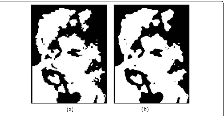
The homotopic alternating sequential filter is a com-position of homotopic cuttings and fillings by balls of increasing radius. It takes an original image X and a control image C as input, and smoothes X while respecting its topology and geometrical constraints implicitly represented by C. A simple illustration is given by Figure 1. Smoothed image (b) is obtained using HAS filter with a radius equal to five and four connect-edness (Γ4). More example can be found in [5].

Based on this filter, Authors [5] introduce a general smoothing procedure with a single parameter to control smoothing degree. LetC⊆X, rÎ Nand D⊆XwithX any finite subset of E. The homotopic alternating sequential filter (HASF) of order n, with constraint sets CandD, is defined as follows:

HASFC,D

n =HFDn ◦HCCn◦...HFD1 ◦HCC1

In the previous formula, HCC

n (i) refers to homotopic

cutting of X by Bn with constraint set C and HFDn(ii)

refers to homotopic filling of X byBnwith constraint

setD. These two homotopic operators can be defined as follows:

HCC_n(X)=∗H(Y,V)With

Y=H(X,εn(X)∪C)

V=(δn(Y)∩X) (i)

HFD

n (X)=H(Z,W)With

Z=∗H(X,δn(X)∩D)

W=(εn(Y)∪X) (ii)

We recall that H(Z,W) is an homotopic constrained thinning operator. It gives the ultimate skeleton of Z constrained byW. The ultimate skeleton is obtained by selecting simple point in increasing order of their dis-tance to the background thanks to a pre-computed Euclidian distance map [10]. We recall also that *H(Y, V) is an homotopic constrained thickening operator. It thickens the set of Y by iterative addition of points which are simple for Yand belong to the setV until stability.

(3)

3. Parallelization Strategy

In this section, we start by defining the class of topologi-cal operators. We also present our motivation to paralle-lize these algorithms on parallel shared memory machines. Then, we will introduce different steps of our approach after making a brief classification over existing strategies. We will focus especially on distribution phase and tasks scheduling over different processors. Schedul-ing and mergSchedul-ing algorithms are presented and discussed. To illustrate both algorithms, scenarios are also intro-duced and discussed.

3.1 Class of topological algorithms

In 1996, Bertrand and Couprie [11] introduced connectivity numbers for grayscale image. These numbers describe locally (in a neighborhood of 3 × 3) the topology of a point. According to this description any point can be character-ized following its topology. They also introduced some elementary operations able to modify gray level of a point without modifying image topology. These elementary operations of point characterization present a fundamental link between large class of topological operators including, mainly, skeletonization and crest restoring algorithms [12]. This class can also be extended, under condition, to homo-topic kernel and leveling kernel transformation [13], topo-logical watershed algorithm [14] and topotopo-logical smoothing algorithm [5] which is the subject of this article. All men-tioned algorithms get also many algorithmic structure simi-larities. In fact associated characterizations procedures evolve until stability which induce common recursion between different algorithms. The grey level of any point

can also be lowered or enhanced more than once. Finally, all mentioned algorithms get a pixel’s array as input and output data structure. It is important to mention that, to date, this class has not been efficiently parallelized like other classes as connected filter of morphological operator which recently has been parallelized in Wilkinson’s work [15]. Parallelization strategy proposed by Seinstra [16] for local operators and point to point operators can also be cited as example. For global operators, Meijster strategy [17] shows also consistence. Hence the need of a common parallelization strategy for topological operators that offers an adapted algorithm structure design space. Chosen algo-rithm structure patterns that will be used in the design must be suitable for SMP machines.

In reality, although the cost of communication (Memory-processor and inter-(Memory-processors) is high enough, shared memory architectures meet our needs for different reasons: (i) These architectures have the advantage of allowing immediate sharing of data with is very helpful in the conception of any parallelization strategy (ii) They are non-dedicated architecture using standard component (proces-sor, memory...) so economically reliable (iii) They also offer some flexibility of use in many application areas, particular image processing.

3.2 Split Distribute and Merge Strategy

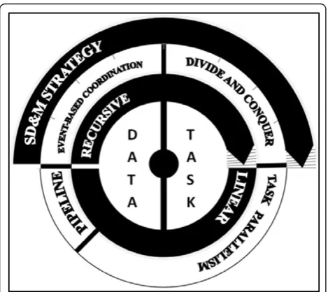
In practice, most effective parallel algorithm design might make use of multiple algorithm structures thus proposed strategy is a combination of the divide and conquer pat-tern and event-based coordination patpat-tern, see Figure 2. Hence the name that we have assigned: SD&M (Split

(a) (b)

(4)

Distribute and Merge) strategy. Not to be confused with mixed-parallelism approach (combining data-parallelism and task-parallelism), it is important to mention that our strategy (i) represents the last stitch in the decomposition chain of algorithm design patterns and it provides a fine-grained description of topological operators paralleliza-tion while mixed-parallelism strategy provides a coarse-grained description without specifying target algorithm. (ii) It covers only the case of recursive algorithms, while mixed-parallelization strategy is effective only in the lin-ear case. (iii) It is especially designed for shared memory architecture with uniform access.

3.2.1 Split phase

The Divide and Conquer pattern is applied first by recur-sively breaking down the problem into two or more sub-problems of the same type, until these become simple enough to be solved directly. Splitting the original problem take into account, in addition to the original algorithm’s characteristics (mainly topology preservation), the mechanisms by which data are generated, stored, trans-mitted over networks (processor-processor or memory-processor), and passed between different stages of computation.

3.2.2 Distribute phase

Work distribution is a fundamental step to assure a perfect exploitation of multi-cores architecture’s potential. We’ll start by recalling briefly some basic notion of distribution techniques then we introduce our minimal distribution approach that is particularly suitable for topological recur-sive algorithms where simple point characterization is necessary. Our approach is general and applicable to shared memory parallel machines. Critical cases are also introduced and discussed.

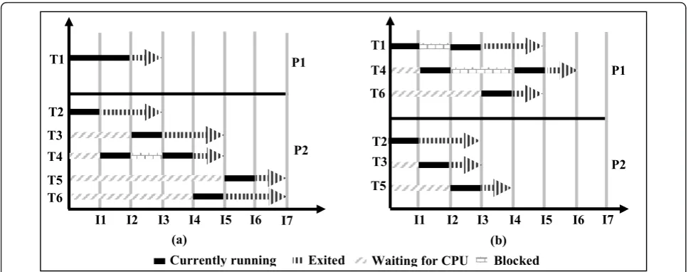
Indeed there are two main types of scheduler. There are those designed for real-time systems (RTS). In this case, the most commonly approaches used to schedule real-time task system are: Clock-Driven, Processor-Sharing and Priority-Driven. Further description of dif-ferent scheduling approaches can be found in [18-20]. According to [20] the Priority-Driven is far superior the other approaches. These schedulers must provide an operational RTS: completed work and delivered results on a timely basis. Other schedulers are designed for Non Real-time system. In this case, schedulers are not subject to the same constraints. Thus,“Symmetric Multiproces-sing”scheduler distributes tasks to minimize total execu-tion time without load balancing between processors, see Figure 3(a). On multi-core architectures, this can lead to high occupancy rate of one processor while the others are free.

We propose a novel tasks scheduling approach to pre-vent improper load distribution while improving total execution time, see Figure 3(b). In literature, there are several schedulers that provide a balanced distribution of tasks such as RSDL “Rotating Staircase Deadline”[21] which incorporates a foreground-background descending priority system (the staircase) with run-queue managing minor and major epochs (rotation and deadline). Other scheduler, as CFS“Completely Fair Scheduler” [22], shows consistence. It handles resource allocation for executing processes, and aims to maximize overall CPU utilization while maximizing interactive performance. These schedulers are based on tasks uniformity principle. Through the tasks homogeneity, better distribution can be achieved and total execution time reduced. Unfortu-nately, these schedulers are not available in all operating system versions especially for small system. Based on the same principle of tasks uniformity, we propose a new scheduling algorithm, simpler to implement and more adapted to topological algorithm implementation.

Let be a basic non-preemptive scheduler‘Basic-NPS’, T= {t1,t2,...,tk} is the set of all tasks,TT= {t1,t2, ...,ti} is

the set of tasks to process withTT⊂T,P= {p1,p2,...,pn}

is the set of all processors andPa= {p1,p2,...,pj} is the set

of available processors withPa⊂P.

Basic-NPS (Tx⇒Py) is able to schedule a set ofTxtasks

onPyprocessor. Let {p} be the maximum of processors

thatPywill contain. Then {p} can be defined as the

maxi-mum of available processors already defined by the setPa

and {p} = maxpj/pjÎPa. While ([Pa≠∅]∧[TT≠∅]) then

Tx⇒Py:TxÎTT;PyÎPa. In this scheduler, each

proces-sor will treat at maximum m= maxti/ti→pj≤max(|

T|

|P|) tasks withjÎ{1, 2,...,n}. Then, the worst case to process

T isK(T) = max

max

i TT→p1, ..., maxj<...<iTT→pk

. As

proof, let suppose that it exist a set L(T) as

(5)

. As‘Basic-NPS’manageL(T) andK(T), so we can intro-duce the following: |L(T)|≤mand |K(T)|≤m. Thus, if

( L(T)≥ K(T))then there exists at least one task {l}, withkÎK(T), such as: (A∧B∧C) withA= (lÎL(T)),B = (l∉K(T)), C = (l>k). This is impossible according to the definition ofK(T) which was defined as the worst case.

Algorithm 1 describes ‘Basic-NPS’ policy. The first step consists on asking operating system to determine the number of available processor. Depending on this number, algorithm will generate process. One active process will be assigned for each available processor. These new processes will belong to the SHED_FIFO class in order to ensure preemption and especially to avoid context switching. Process will only stop running if work is complete or less frequently when another pro-cess, belonging to the same class, with higher priority requesting processor. The global execution will stop if there no more task to process.

3.2.3 Merging phase

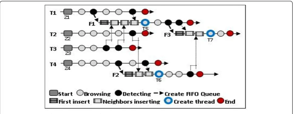
The key problem of each parallelization is merging obtained results. Normally this phase is done at the end of the process when all results are returned by all threads what usually means that only one output variable is declared and shared between all fighting threads. But as we mentioned in section 3.1, we are dealing with a dynamic evolution and if we take into account different steps of simple point detection then pixel characterizations, we can plan the following: The original shared data structure, con-taining all pixels, is divided intonresearch zones {z1,z2..., zn}. We associate one thread from the following list {T1,

T2,...,Tn} to each zone. Each thread can browse freely its zone and if it detects target pixel types, it lowers character-ized pixel and it pushes its eight neighbors in one of the available FIFO queues. A queue is said available if only one thread (owner) is using it. One queue cannot be shared by

more than two threads so if no queue is available, threads can create a new one and become owners.

Since two threads finished, they directly merge and a new thread is created and then same process is lunched again. New created thread will inherit queue shared between his parents. Thus it can restart research. It is also important to mention that there is no hierarchical order in thread mer-ging, only criteria is finishing time. We mention also that one neighbor cannot be inserted twice. It is a precaution in order to minimize consumed cache. More formal descrip-tion of merging techniques is given in by algorithm 2.

It is important to highlight similarity and difference that may exist between our merging algorithm and KPN [23]. In effect, both are deterministic and do not depend on execution order. But KPN algorithm may be executed in sequentially or in parallel with the same outcome while our merging algorithm is designed only for parallel execu-tion. KPN support recurrence and recursion while our merging algorithm support only recursion.

In large scale application, KPN showed consistence. Examples include Daedalus project [24] where generated KPN models are used to map process into FPGA architec-ture. Ambric architectures [25] implement also a KPN model using bounded buffers to create massively DMP Machines based on structural object programming model.

In a narrower framework limited to simple point char-acterization, the implementation of such a model will be very expensive and it would be better to find an easier and more specific algorithm.

In Figure 4, we give an illustration of the merging algo-rithm with four threads. The original shared data structure is divided into 4 research areas {z1,z2,z3,z4}. Threads {T1, T2,T3,T4} will start browsing different zones in parallel.T1 is the first to detect target point (constructible, destructi-ble...) so it lowers characterized pixel (inz1) and it pushes

I1 I2 I3 I4 I5 I6 P1

P2 T1

T2 T3

I1 I2 I3 I4 I5 I6

P1

P2 T4

T3 T5

Waiting for CPU T1

T6

T2

Blocked T4

T5 T6

Currently running Exited

I7

(a) (b)

I7

(6)

its eight (or four) neighbors in FIFO queueF1that it has created before continue browsing. Later,T3will detect new target point so it will lower characterized pixel (inz3) then push neighbors inF1before continue browsing.T3does not need to create new FIFO queue sinceF1is available.T1 andT3will repeat this procedure twice. Since they finish browsing, they merge and new threadT5is born.T5will start browsing onlyF1. Since it detect new target point so it will lower characterized pixel (inz5=z1+z3) then push neighbors inF3that it has created before continue brows-ing. SimilarlyT2andT4will generate the creation ofF2and T6. HereT6will eventually merge withT5to give birth to T7. Finally there will be a single threadT7which will brows F3without detection any target points.

We have introduced, in this section, three necessary steps to implement our parallelization strategy (SDM). It is important to mention that some similarity may exist between our split/merging phases and alpha-extension/ beta-reduction phases from structural perspective. Actu-ally both approaches intended to put in place more guar-antees that the parallelism will actually be met. But uses contexts are different. In effect, Jean Paul Sansonnet [26-28] team introduced alpha-extension (diffusion) and beta-reduction (merging) notions for stream manipulation in the framework of Declarative Data Parallel language definition and there techniques cannot be applied without a scalar function. While our proposal is restricted to topo-logical characterization in the framework of topotopo-logical operator’s parallelization and no scalar function is required during the application of these two phases.

4 Parallel smoothing filter

In this section we start by analyzing overall structure of original algorithm. Then we continue with the paralleliza-tion of Euclidean distance, thinning and thickening algo-rithm. We conclude by a performance analysis of the

entire smoothing topological operator. Obtained execu-tion time, efficiency, speedup and cache misses will be introduced and discussed.

As we have shown in Section 2, smoothing algorithm receives as input a binary image and maximum radius. It uses two procedures for homotopic opening and closing, see Figure 5(a) (b). The call is looped to ensure an ongoing relationship between input and output. The opening pro-cess is a consecutive execution of erosion, thinning, dilata-tion and thickening. While closure procedure ensures the same performance of the four consecutive functions with single difference: the erosion instead of dilatation. Thin-ning and thickeThin-ning ensure the topological control of ero-sion and dilatation. This control is based on researching and removing of all destructible points. When destructible point is deleted, its neighbors are reviewed to ensure that they are not destructible either.

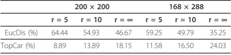
A preliminary assessment of first implementation code, see Table 1, shows that Euclidean distance computing (EucDis) takes more time than topological point character-ization (Topcar). For an image of (200*200), computation time of Euclidean Distance (E.D) with an infinite radius is 46.67% while point characterization of 2.4 million points occupies only 18.15%. If we limit radius between 5 and 10, computation time of (E.D) continues to increase. It can reach 64.44% of total time with a radius equal to 5. How-ever time for topological characterization is only 8.89% for 1 million points. These finding remain the same if we increase image size. Beyond (512*512), computing time of point characterization becomes considerable.

4.1 Euclidean distance computing

4.1.1 Study on Euclidian Distance algorithms

During previous evaluation, 4SED [10] algorithm was used for Euclidean distance computation. So we are looking for another algorithm that is faster, and

(7)

parallelizable. New algorithm must have an Euclidean distance computation error less than, or equal to, that produced by 4SED in order to maintain homotopic characteristics of the image. In literature, several algo-rithms for Euclidean distance computing exist. Lemire [29] and Shih [30] algorithms are bad candidates because Lemire’s algorithm does not use Euclidean cir-cle as structuring element. Then homotopic property will not be preserved. Shih’s algorithm has a strong data dependency which penalizes parallelization. In [31], Cuissenaire propose a first algorithm for Euclidian dis-tance computing, called PSN“Propagation Using a Sin-gle Neighborhood” that uses the following element structure:

d4(p) =

q∨qx−px

2

+qy−px

2 <1

(ia)

He also proposes a second algorithm, called PMN

“Propagation Using Multiple Neighborhood” that uses eight neighbors. In [32], he also proposes a third algo-rithm with o(n3/2) complexity, which offers an accurate computation of the Euclidean distance. Only drawback of this third algorithm is computation time which is very important and goes beyond the two algorithms

mentioned above. Even if computing error produced by PSN is greater than computing error produced by PMN, it is comparable to that produced by 4SED. Low data dependence and ability to operate on 3D images, makes PSN algorithm a potential candidate to replace 4SED.

Meijster [17] proposes an algorithm to compute exact Euclidean distance. Algorithm complexity iso(n) and it operates in two independent, but successive, steps. First step is based on looking over columns then computing distance between each point and existing objects. Second step includes same treatment looking over lines. It is important to note that strong independence between dif-ferent processing steps and computing error equal to zero makes Meijster algorithm another potential candi-date to replace 4SED. Algorithm is also able to operate on 3D images. Theory analysis of Meijster and Cuisse-naire algorithms can be found in Fabbri’s work [33].

In the following, we propose first analysis based on dif-ferent algorithms implementation in order to compare between them. We have implemented 4SED algorithm using a fixed size stack. This stack uses a FIFO queue and it has small size while 4SED algorithm does not need to store temporal image. Results are directly stored into the output image, we will retain this implementation because 4SED assessment serve only as reference for comparison. For PSN implementation, we used stacks with dynamic sizes. Memory is allocated using small blocks defined at stack creation. When an object is added to queue, algorithm will use available memory of last block. If no space is available, a new block is allocated automatically. Block size is proportional to image size (N × M/100). Finally we used a simple memory structure to implement Meijster algorithm. A simple matrix was used

Homotopic Alternating Sequential

Filter

Homotopic

Closing (b)

Homotopic

Opening (a)

Erosion

Thinning

Dilation

Thickening

Erosion

Thinning

Dilation

Thickening

Figure 5Overall structure of the original smoothing algorithm.

Table 1 Time execution rate of E.D and topological characterization functions

200 × 200 168 × 288

r = 5 r = 10 r =∞ r = 5 r = 10 r =∞

EucDis (%) 64.44 54.93 46.67 59.25 49.79 35.25

(8)

to compute distance between points and object of each column and three vectors were used to compute distance in each line. We recall that this comparison is done in order to select the best algorithm among three candidates.

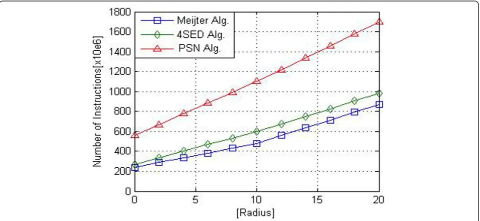
Figure 6 describes obtained results by different imple-mentations on single processor architecture P4. During this evaluation we used binary test image (200 × 200). We have also varied ball radius. We used Valgrind software to evaluate different designs. Callgrind tool returns the cost of implementing of each program by detecting IF (Instruc-tion Fetch). Results show that PSN algorithm is the most expensive in all cases (for any radius). Meijster algorithm is moderately faster than 4SED. The output images returned by Meijster algorithm hold the best visual quality while Euclidean distance computation error is almost zero thus our efforts will be brought on Meijster algorithm parallelization.

4.1.2 Parallelization of Meijster algorithm

We denote by I input image with m columns and n rows. We denote byBan object included inI. The idea is to compute, for each pointpÎ I∧p∉B, separating distance betweenpand the closest point b with b Î B and∀(0 ≤b≤m),b = (bx,by). This amount to compute

the following matrix:

dtpx,py

=EDT(p) withEDTp= minpy−bx

2

+Gpx,by

2

.

If we assume that minimum distance of an empty group Kis∞and ∀z Î K, we have (zy +∞) =∞ then

EDT(p) formula can be written as follow: ∀bx <n,∀by≤

m, EDT(p) = min(py-bx)2+G(px, by)2 with G(px, y) =

min|px-bx|:b= (bx,y).

Thus we can split the Euclidian distance transform procedure into two steps. The first step is to scan col-umns and compute EDT for each column y. Second step consists on repeating the same procedure for each line. In the following we start by detailing these two steps: In the first stepG(px,y) can be computed through

the two following sub functions:GT(px,y) = minpx-bx:b

= (bx,y), GB(px,y) = minbx-px: b= (bx,y) with ∀0 ≤bx

≤ n. To computeGT(px, y) andGB(px,y), we scan each

column y from top to bottom using the two following formula: GT(px,y) =GT(y, px-1)+1,GB(px,y) = GB(y,px

-1)+1. Thus sequential algorithm of the first step can be written as follows. The complexity order iso(n×m).

Let’s move to the second step. We start by defining f (p, y) = (py-y)2+G(px, y)2. Then we can defineEDT(p) =

min f(p-y), ∀0 ≤ y ≤ m. For each row u, we note that there is, for the same point p, the same value off(p,y) for different values of y, so we can introduce the con-cept of“region of column“.

LetS be the set ofy points such thatf(p,y) is minimal and unique. The formula of S, ∀0 ≤ y ≤ u, is Sp(u) =

min y: f(p, y)≤f(p,i). ∀0≤i ≤u∧u ≤m. LetT be the set of points with coordinate greater than, or equal to, horizontal coordinate of the intersection with a region: Tp(u) =Seppx(Sp(u−1),u) + 1.

Let Sep(i, u) be the separation between regions of i andu, defined by:

f(p,i)≤f(p,u)⇔(py−i)2₊_G(px,_i)2_≤_(py₋_u)2₊_G(px,_u)2_⇔_Sepp x(i,u) = (u2₋_i2₊_Dif_)/2(u₋_{1) =}_py_With_Dif_{= (G(px,}_u)2₋_G(px,_i)2_).

Thus lines will be processed, from left to right then from right to left. During the first term, from left to

(9)

right, two vectors S and T will be created. These two vectors will contain respectively all regions and all inter-sections. During the second treatment, from right to left, we computeffor each value ofS.fis also computed for each respective values of T. Algorithm 4 is asso-ciated to second step. For the first term, complexity order is q+2(m-u) whereas complexity order of the sec-ond term is onlym.

The independence of data processing between rows and columns is the key to apply of SDM parallelization strategy. In the first stage, column processing, we can define data interdependence by the following equation:

Gpx,y= minGT

px,y,GB

px,y⇔GT

px,y=

0 if(px,y)∈B GT

px,yelse

⇔GB

px,y= minGB

px+ 1,y,GT

px,y

It follows that values of each column y of G, depends only on lines: px,px+1 andpx-1. Similarly, at the second

stage, we can introduce the following interrelationship: Edt(p) =f(p, Sp(q)).

Then∀(0≤ y ≤u), (0≤i ≤u)Λ(u <m),Sp(u) = min

y:f(p,y)≤f(p,i). Thus, if (u=Tp(q)) soq= (q-1) which

imply the following: Tp(u) =Seppx(Sp(q),u) + 1.

According to this formalization, values off(p,i) and Sepx(i,u) are independent of modified data. So using two

vectorsSandT, a private variableqfor each line ensures complete independence in writing. We start applying the splitting step by sharing the columns and lines processing between multiple processors. A thread can process one or more columns and the number of threads used will depend on the number of processors. The results returned by all threads in this first stage will be merged in order to start lines processing. In the following we introduce the parallel version of Meisjter algorithm for both steps. Associated algorithm complexity iso((n × m)/

N). (n×m) refers to image size andNrefers to the num-ber of processors.

Proposed parallel version of Meijster algorithm was implemented in C using OpenMP directives. Speedup for numbers of threads equal to 1, 2, 4, 8, and 16 were determined. The efficiency measure Ψ (n) is given by the following formula withn the number of processors: Ψ(n) = seq. time/(n*para. time) (ii)

Times were performed on eight-core (2× Xeon E5405) shared memory parallel computer, on Intel Quad-core Xeon E5335, on Intel Core 2 Duo E8400 and Intel mono-processor Pentium 4 660. The minimum value of 5 timings was taken as most indicative of algorithm speed. More information about architectures character-istics are given in Section 4.

The measurements were done on 2D binary image (512*512). If we can get a satisfactory outcome for this standard, it will be the same for smaller size images. View cache size limits, larger image will not be tested. Figure 7 shows that number of instructions to compute Euclidian distance drops from an average of 9.5 × 108using 4SED algorithm down to 7.6 × 108ms with Meijster algorithm. Despite the passage from a sequential version running on single core to a parallel version running on 8 processors, acceleration is only multiplied by 1.6 as shown in Figure 8 (a). This can be explained by the choke point between col-umns processing and lines processing. Waiting time between these two treatments significantly penalizes accel-eration. Figure 8(b) shows that efficiency variation depends on the number of threads. It is also proportional to the number of processors. Moving to 3, 5 or 7 threads (odd number) decreases significantly the efficiency which reaches its maximum each time that the number of threads is equal the number of processors.

(10)

4.2 Thinning and thickening computing

Algorithms of thinning and thickening are almost the same. The only difference between them is the follow-ing: in thinning algorithm, destructible points are detected then their values are lowered. In thickening algorithm, constructible points, are detected then their values are increased. For parallelization, we will apply the same techniques introduced in [34]. We propose a similar version using two loops. Target points are initi-ally detected then their value lowered or enhanced according to appropriate treatment. The set of their eight (or four) neighbors are copied into a “buffer” and rechecked. This treatment is repeated until stability. In the following, we present an adapted version of Coup-rie’s thinning algorithm.

Unfortunately direct application of introduced parallel processing is not possible with the set of all points. Some points, called critical points, cannot be eliminated in parallel because initial topology of the image may be broken. Figure 9 illustrates this case: Critical points of

an input image (a) are identified in (b). If these points are deleted in one iteration (c) topology necessary is broken (d).

To resolve this problem, we propose that research areas assigned to each thread must be composed of at least six lines (of the image). Each thread will use two buffers to treat each three lines thus four buffers are used to treat six lines as shown in Figure 9(e).

Through this organization threads can start running in parallel on Z11, Z21and Z31. Once processing is com-pleted threads can restart running on Z12, Z22and Z32. In some cases, a neighbor of a destructible point is detected on the border of a contiguous area. To prevent that such neighbor escape to recheck, it must be injected to buffer of the right thread. Let’s suppose that a pointpÎZ2is considered as destructible by T2, so its value will be low-ered and its four neighbors {v1,v2, v3, v4} should be rechecked. Neighbors {v1,v2,v4} belong to Z2so they will be push in T2 buffers. The neighbor {v3} belongs to Z3so it will stack T3 buffers.

(a) (b)

Figure 8(a) Performance evaluation (b) Efficiency evaluation [Meisjter Algorithm].

X

0 0 0 0 0

(a)

X

0 0 0 0 0

0

0 0 0

0 (b)

0 0 0 0 0

X

(c) 0 0 x0 0 0

(d)

Z11

Z12

Z21

Z22

Z31

Z32

3 Lines

Critical frontiers

(11)

Performance evaluation of introduced adapted version of Couprie’s algorithm is shown in Figure 10. On eight cores architecture, acceleration does not exceed 3.4. Such moderate result can be explained by critical bor-ders processing. Regarding efficiency, the best perfor-mance is achieved when the number of thread is equal to the number of processors. If this equality is not ensured, the efficiency decreases. The problem threads’ add number still persists.

The next step is to combine the parallel version of Meijster algorithm and the adapted version of Couprie algorithm to build the parallel processing of topological smoothing.

4.3 Global analyses

In this section, we present a global evaluation of the parallel smoothing operator. We start by presenting per-formance evaluations in terms of acceleration and effi-ciency. Then, we evaluate cache memory consumption.

4.3.1 Execution time

We implemented two versions of the proposed parallel topological smoothing algorithm, the first one using

‘Symmetric Multiprocessing’scheduler and the second one using ‘basic-NPS’ scheduler. Wall-clock execution times for numbers of threads equal to 1, 2, 4, 8, and 16 were determined. The minimum value of 2 timings was taken as most indicative of algorithm speed. The mea-surements were done on 2D binary image (512*512). Results of the second implementation on the eight-core are shown in Figure 11.

We note that number of instructions drops from an average of 1879 × 108FI with a single thread down to 1652 × 108ms with 8 threads. As expected, the speed-up for the second implementation using‘basic-NPS’scheduler is higher than for the one using“Symmetric Multiproces-sing”scheduler, thanks to balanced distribution of tasks.

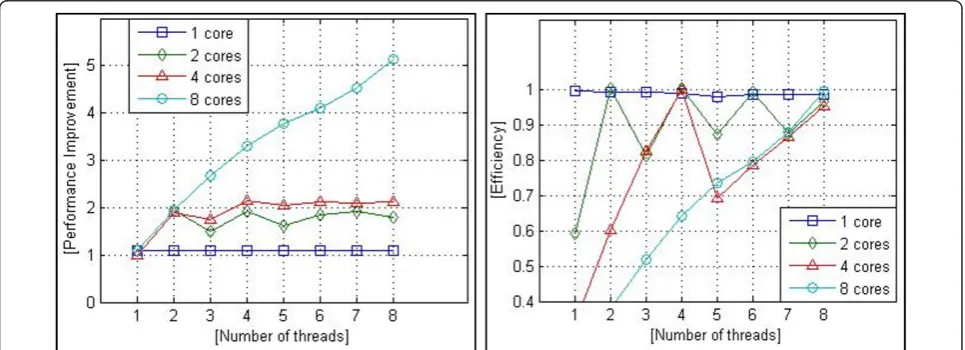
A remarkable result about speedup is also shown in Figure 12(a). In fact, speed-up increases as we increase the number of threads beyond the number of processors in our machine (eight cores). In the first implementation, using“Symmetric Multiprocessing”scheduler, the speedup at 8 threads is 1.9 ± 0.01. However, for the second imple-mentation, using our scheduler, the speedup has increased to 5.2 ± 0.01. Another common result between different architecture is stability of execution time on each n-core machine since the code uses n or more threads.

For better readability of our results, we tested also efficiency of our algorithm on various architectures (see Figure 12(b)) using the ψ(n) formula introduced earlier. For parallel time ratio we used best obtained time with 8 threads (’basic-NPS’scheduler).

4.3.2 Cache Memory Evaluation

As memory access is a principal bottleneck in current-day computer architectures, a key enabler for high perfor-mance is masking the memory overhead. If we starts from basic theory that two classic cache design parameters dra-matically influence the cache performance: the block size and the cache associativity. So the simplest way to reduce the miss rate is to increase the block size even it increases the miss penalty. The second solution is to decrease asso-ciatively in order to decrease hit time thus to retrieve a block in an associative cache, the block must be searched inside of an entire set since there is more than one place where the block can be stored.

Unfortunately, we are dealing with non-reconfigurable architectures with caches whose associativity and block size are predefined by the manufacturer. Nowadays, new approaches to reduce cache miss are developed such as taking advantage of locality of references to memory or using aggressive multithreading so that whenever a thread is stalled, waiting for data, the system can efficiently switch to execute another thread. Despite their power, the

(a) (b)

(12)

application of both approaches remains limited. In fact, applications of locality approach still experimental even with Larrabee technology introduced by Intel. And the aggressive multithreading approach has been specially designed for graphics processing engines, which manage thousands of in-flight threads concurrently. So it is not recommended for general SMP machines with limited number of processors and threads. With all these limita-tions, the most intuitive solution is to rely on the schedul-ing. Thanks to our basic-NPS scheduler, we have balanced the charges then prevent context switching thus we mini-mize caches misses.

In the following we present our experimental analysis. We consider a commonly used Intel processor configura-tion (More details are given by table 2). Number of pro-cessor varies from one to eight. The frequency varies between 1,73 GHz and 3,4 GHz. The L1 caches have at least a 32-byte block size, while capacity vary between 16

Kbytes and 32 Kbytes, and for the associativity, only eight ways is considered. The L2 caches have at least a 64-byte block size, while capacities vary between 512 Kbytes and 6 Mbytes, and the associativity varies between two and twenty four ways.

The scheduler relies on our basic-NPS scheduling policy. As a result of this experiment, see Figure 13(A-1), we found that three performance regions are clearly evident: In the leftmost region, as long as the cache capacity can effectively serve the growing number of threads, increasing the number of threads improves performance, as more processors are utilized. This area is generally identified as cache-efficiency zone. At some point, the cache becomes too small for the growing stream of access requests, so memory latency is no longer masked by the cache and instruction cache misses reduce more moderately. As the number of available threads again increases, the multi-thread efficiency zone (on the right) is reached, where

Figure 11Number of instructions & tasks distribution using‘Basic-NPS’.

(13)

adding more threads improves performance up to the maximal performance of the machine, or up to the band-width wall. Balanced workloads offer higher locality and better exploit the cache and hence expand the cache effi-ciency zone to the right and up. An outstanding example is given by table 3 which summarizes number of L1 instruction misses on Intel Dual Core T1400 architecture using SMP scheduling policy and Basic-NPS scheduling policy. We note that number of instruction misses drops from an average of 18844 L1 Instr. misses (using SMP) with two threads down to 6030 L1 Instr. misses (using Basic-NPS) usually with two threads. Here success rate is largely above the average of 50%. The same rate will be practically maintained when increasing the number of threads (Figure 14).

Moreover, the shape of the performance curve depends on how fast the cache hit rate degrades as a function of the number of threads. Any success access to L1 will elim-inate an attempt to access to L2 thus performance curve, Figure 15, will evaluate in the same way. By reducing the number of cache miss from instruction cache, processor or thread of execution has not to wait (stall) until the instruction is fetched from main memory which immedi-ately impact execution time.

Figures 14(A) and 16(A-1) show so much load balancing and implicitly context switching between processes can affect performance in terms of reading data from caches. However, improvement in writing data, see Figure 14(B) and Figure 16(B-1), in two caches remains modest. When there are more computation instructions per memory

Table 2 Hardware configuration

Intel P4

Intel Dual Core T1400

Intel C2 Quad Q9550

Intel Xeon E5405

Number of processor 1 2 4 2 × 4

SMT Yes Yes Yes Yes

Frequency 3,4 GHz 1,73 GHz 2,83 GHz 2,00 GHz

L1 Instruction Cache Size 16 Kb 32 Ko 32 Ko 32 Ko

Asso. 8-way 8-way 8-way 8-way

Block size 32 byte 32 byte 32 byte 32 byte

L1 Data Cache

Size 16 Kb 32 Ko 32 Ko 32 Ko

L2 Cache

Size 2 Mb 512 Kb 6 Mb 6 Mb

RAM size 1 Gb 2 Gb 2 Gb 8 Gb

(14)

access, performance climbs more steeply with additional threads. This is because as more instructions are available for each memory access, fewer threads are needed to fill the stall time resulting from waiting for memory.

5 Conclusion

Topological characteristics are fundamental attributes of an object. In many applications, it is mandatory to pre-serve or control the topology of an image. Nevertheless, the design of transformations which preserve both topolo-gical and geometrical features of images is not an obvious task, especially for parallel processing.

In this paper, we have presented a new parallel com-putation method for topological smoothing through combining parallel computation of Euclidean Distance Transform using Meijster algorithm and parallel Thin-ning-Thickening processes using an adapted version of Couprie’s algorithm.

We have also presented a new parallelization strategy called SDM (Split Distribute and Merge). Proposed strategy is partially based on divide and conquers principle asso-ciated to event-based coordination techniques. Further than smoothing operator, SDM Strategy can be applied for a large class of topological operators as we shown in section 3.1. In addition to identified conditions during splitting step, we introduced an adapted scheduler called basic-NPS (Basic - Non Preemptive Scheduler) able to distribute in balanced way a set of active tasks on available processors. Finally we introduced an adapted merging policy designed especially for dynamic system evolving until stability.

Parallel topological operator computation poses many challenges, ranging from parallelization strategies to implementation techniques. We tackle these challenges using successive refinement, starting with highly local operators, which process only by characterizing points and then deleting target pixels, and gradually moving to more complex topological operators with non-local behavior. In future work, we will study parallel computation of the topological watershed [14].

Algorithm 1. Scheduling policy

1.T: Set of all tasks 2.P: Set of all processors 3. While (T≠∅) repeat: 4. NT= Nbr_active_tasks();

5. NP= Nbr_ available_processors();

6. If (NP≠0) then

7. If (NT<NP) then

8. For each processorNpi:

9. Generate-new-process (NTi);

10. Identify-class (NTi, SCHED_FIFO);

11. Endfor

12. Else:NDT= Desable_tasks (NP-NT);

13. Insert_desabled_tasks (NDT, T);

14. For each processor NPi:

15. Generate-new-process (NTi);

16. Identify-class (NTi, SCHED_FIFO);

17. Endfor 18. EndIf 19. EndIf

Table 3 L1 - Instructions Misses (Symmetric Multiprocessing scheduler vs.Basic-NPS scheduler)

Number of threads 2 3 4 5 6 7 8

Instruction L1 misses

SMP Scheduler

18844 19476 18638 19726 20058 20324 18946

Basic-NPS scheduler 6030 6262 6035 6437 7202 7804 7085

(15)

20. EndWhile

Algorithm 2. Merging technique

1. Z: Set of research zones 2. T: Set of threads

3. FIFO_Q: Set of available FIFO queues 4. PT: Target pixel type;PD: Detected pixel

5. For all zones (ZiÎZ) do:

6. Parallel_browsing (Ti,Zi);

7. EndFor

8. For each thread (TiÎ T) do:

9. If (pixel_caract(Ti,PT)==True) then

10. modify_value(PD);

11. If ((FIFO_Q≠∅) then 12. usedstatus(FIFO_Qj, true);

13. insert_neighbors(Ti, PD,FIFO_Qj);

14. Else: add_new_fifo (FIFO_Q) 15. usedstatus(FIFO_Qj+1, False); Figure 15Instruction - L2 misses (B): zoom on (A).

(B-1) (B-2) (A-2) (A-1)

(16)

16. insert_neighbors(Ti, PD,FIFO_Qj+1); 17. EndIf;

18. EndIf; 19. EndFor;

Algorithm 3. Meijster original version [1st Step]

1. Data: m:colums, n:lines, b:image 2. ForallyÎ [0..m-1] do

3. If (0,y)ÎBtheng[0..y] = 0 4. elseg[0..y] =∞

5. endif 6. /* GT*/

7. for (x= 1) to (n-1) do 8. if [x,y]ÎBtheng[x..y] = 0 9. elseg[x,y] =g[x+1,y]+1 10. endif

11. endfor 12. /* GB*/

13. for (x=n-2) downto (0) do 14. ifg[x+1,y] <g[x,y] then 15. g[x,y] =g[x+1,y]+1 16. endif

17. endfor 18. endforall

Algorithm 4: Meijster original version [2nd Step]

1. Data: b:image, g: G_Table, m: columns, n:lines 2. ForallxÎ[0..n-1] do

3. q= 0 4. s[0] = 0 5. t[0] = 0 6. /* First part */

7. for (u= 1) to (m-1) do

8. A= (q≥0)Λ[f((x,t[q]),s[q])] 9. B=f((x,t[q]),u)

10. while (A>B) thenq¬(q+1) 11. end while

12. if (q < 0) then (q¬ 0) 13. (s[0]¬u)

14. elsew¬Sep(s[q],u,x)+1 15. if (w<m) thenq ¬(q+1) 16. s[q]¬u

17. t[q]¬w

18. endif

19. endif 20. endfor

21. /* Second part */ 22. for (u=m-1) to (0) do 23. Edt[x,u] =f((x,u),s[q]) 24. if (u=t[q]) thenq¬ (q-1) 25. endif

26. Endfor 27. End forall

Algorithm 5. Meijster parallel version [1st step]

1. For (y=t,y<m,y =y+tmax) do 2. If (0,y)ÎBtheng[0,y]¬ 0 3. elseg[0,y]¬∞

4. endif 5. /* GT*/

6. for (x= 1) to (n-1) do

7. if [x,y]Î Btheng[x,y]¬ 0 8. elseg[x,y]¬g[x+1,y]+1 9. endif

10. Endfor 11. /* GB*/

12. for (x=n-2) downto (0) do 13. if (g[x+1,y] <g[x,y]) then 14. g[x,y]¬ g[x+1,y]+1 15. endif

16. Endfor 17. Endforall

Algorithm 6. Meijster parallel version [2nd Step]

1. For (x=t,x<n,x=x+tmax) do 2. q= 0;s[0] = 0;

3. t[0] = 0; 4. /* First part */

5. for (u= 1) to (m-1) do

6. A¬(q≥0)Λ[f((x,t[q]),s[q])] 7. B¬f((x,t[q]),u)

8. while (A>B) doq¬(q+1) 9. end while

10. if (q < 0) then (q¬ 0) 11. (s[0]¬u)

12. elsew¬Sep(s[q],u,x)+1 13. if (w<m) thenq ¬(q+1) 14. s[q]¬u

15. t[q]¬w

16. endif

17. endif 18. Endfor

19. /* Second part */

20. for (u=m-1) downto (0) do 21. Edt[x, u]¬f((x,u),s[q]) 22. if (u=t[q]) thenq¬ (q-1) 23. endif

24. Endfor 25. End forall

Algorithm 7. Adapted version of thinning algorithm

1. while (input[x] is destructible) do 2. push(x,stack1)

(17)

6. While (stack1≠∅)∧(maxiter> 0) do

7. While(stack1≠∅)do 8. x¬ pop(stack1)

9. if (output[x] is destructible) then 10. output[x]¬reduce_pt(x) 11. push(x,stack2)

12. endif 13. end while

14. While (stack2≠∅))do 15. x¬pop(stack2) 16. v¬neighbors(x) 17. i¬0

18. While (i< 8) do 19. if (v[i]∉stack1) then 20. push(v[i],stack1)

21. endif

22. endwhile 23. endwhile

24. maxiter¬ maxiter -1

25. Endwhile

Competing interests

The authors declare that they have no competing interests.

Received: 1 March 2011 Accepted: 27 October 2011 Published: 27 October 2011

References

1. Taubin G:Curve and surface smoothing without shrinkage.Proceedings of ICCV’95, 852-8571999.

2. X Liu, Bao H, Shum H-Y, Peng Q:A novel volume constrained smoothing method for meshes.Graphical Models2002,64:169-182.

3. Asano A, Yamashita T, Yokozeki S:Active contour model based on mathematical morphology.ICPR1998,98:1455-1457.

4. Leymarie F, Levine MD:Curvature morphology.Proceedings of Vision Interface1989, 102-109.

5. Couprie M, Bertrand G:Topology preserving alternating sequential filter for smoothing 2D and 3D objects.J Electron Imaging2004,13:720-730. 6. Yung Kong T, Rosenfeld A:Digital topology: introduction and survey.

Comput Vision Graphics Image Process1989,48:357-393.

7. Sternberg SR:Grayscale morphology.Comput Vision Graphics Image Understanding1986,35:333-355.

8. Serra J:Image Analysis and Mathematical Morphology.InTheoretical Advances. Volume II.Academic Press, New York; 1988, Chap. 10. 9. Bertrand G:Simple points topological numbers and geodesic neighbourhoods in cubic grids.Pattern Recognition Letters1994,

15:1003-1011.

10. Danielson PE:Euclidean distance mapping.Computer Graphics and Image Processing1980,14:227-248.

11. Bertrand G, Everat JC, Couprie M:Topological approach to image segmentation.SPIE Vision Geometry V1996,2826:65-76.

12. Couprie M, Bezerra FN, Bertrand G:Topological operators for greyscale image processing.Journal of Electronic Imaging2001,10:1003-1015. 13. Bertrand G, Everat JC, Couprie M:Image segmentation through operators

based on topology.Journal of Electronic Imaging1997,6:395-405. 14. Bertrand G:On topological watersheds.J Math Imaging Vision2005,

22:217-230.

15. Wilkinson MHF, Gao H, Hesselink WH, Jonker J, Meijster A:Concurrent computation of attribute filters on shared memory parallel machines.

Trans Pattern Anal Mach Intell2007, 1800-1813.

16. Seinstra FJ, Koelma D, Geusebroek JM:A software architecture for user transparent parallel image processing.International Euro-Par conference 2001,2150:653-662.

17. Meijster A, Roerdink JBTM, Hesselink WH:A general algorithm for computing distance transforms in linear time.Mathematical Morphology and its Applications to Image and Signal ProcessingKluwer Academic Publishers, Dordrecht; 2000, 331-340.

18. Natarajan S, ed:Imprecise and Approximate ComputationKluwer, Boston; 1995.

19. Van Tilborg AM, Koob GM, eds:Foundations of Real-Time Computing: Scheduling and Resources Management, Kluwer, Boston1991. 20. Leung J, Zhao H:Real-time scheduling analysis report.Department of

Computer Science New Jersey Institute of Technology2005. 21. Kolivas C:RSDL completely fair starvation free 64 interactive cpu

scheduler.lwn.net2007.

22. Molnar I:Modular scheduler core and completely fair scheduler.lwn.net 2007.

23. Kahn G:The semantics of a simple language for parallel programming.

Proceedings of the IFIP Congress 74North-Holland Publishing Co., Amsterdam; 1974.

24. Nikolov H, Thompson M, Stefanov T, Pimentel AD, Polstra S, Bose R, Zissulescu C, Deprettere EF, Daedalus :Toward Composable Multimedia MP-SoC Design, invited paper.Proceedings of the ACM/IEEE International Design Automation Conference(DAC‘08), Anaheim, USA; 2008, 574-579. 25. Halfhill T:Ambric’s new parallel processor.Microprocessor Report2006. 26. Giavitto J-L, Sansonnet J-P:Introduction à 8 1/2 Rapport interne.LRI Orsay

1994.

27. Giavitto J-L, Sansonnet J-P:8 1/2: data-parallélisme et data-flow.

Techniques et Sciences Informatiques1993,12(5).

28. Mahiout A, Giavitto J-L, Sansonnet J-P:Distribution and scheduling data-parallel dataflow programs on massively data-parallel architectures.SMS-TPE

‘94: Software for Multiprocessors and SupercomputersOffice of Naval Research USA & Russian Basic Research Foundation, Moscow; 1994. 29. Lemire D:Streaming maximum-minimum filter using no more than three

comparisons per element.Nordic J Comput2006,13(4):328-339. 30. Shih FY, Wu Y:Fast Euclidean distance transformation in two scans using

a 3 × 3 neighborhood.Comput Vis Image Understanding2004,94:195-205. 31. Cuisenaire O, Macq B:Fast Euclidean distance transformation by

propagation using multiple neighborhoods.CVIU1999,76(2):163-172. 32. Cuisenaire O, Macq B:Fast and exact signed Euclidean distance

transformation with linear complexity.IEEE International Conference on Acoustics, Speech and Signal Processing (ICASSP99)1999, 3293-3296. 33. FABBRI R, COSTA LF, TORELLI JC, BRUNO OM:2D Euclidean distance

transform algorithms: A comparative survey.ACM Computing Surveys 2008,40.

34. Mahmoudi R, Akil M, Matas P:Parallel image thinning through topological operators on shared memory parallel machines. Signals.Systems and Computers Conference2009, 723-730.

doi:10.1186/1687-5281-2011-16

Cite this article as:Mahmoudi and Akil:Enhanced computation method

of topological smoothing on shared memory parallel machines.EURASIP

Journal on Image and Video Processing20112011:16.