METHODOLOGY
Unsupervised machine learning applied
to scanning precession electron diffraction data
Ben H. Martineau
1*, Duncan N. Johnstone
1, Antonius T. J. van Helvoort
3, Paul A. Midgley
1and Alexander S. Eggeman
2Abstract
Scanning precession electron diffraction involves the acquisition of a two-dimensional precession electron diffrac-tion pattern at every probe posidiffrac-tion in a two-dimensional scan. The data typically comprise many more diffracdiffrac-tion patterns than the number of distinct microstructural volume elements (e.g. crystals) in the region sampled. A dimen-sionality reduction, ideally to one representative diffraction pattern per distinct element, may then be sought. Further, some diffraction patterns will contain contributions from multiple crystals sampled along the beam path, which may be unmixed by harnessing this oversampling. Here, we report on the application of unsupervised machine learning methods to achieve both dimensionality reduction and signal unmixing. Potential artefacts are discussed and preces-sion electron diffraction is demonstrated to improve results by reducing the impact of bending and dynamical diffrac-tion so that the data better approximate the case in which each crystal yields a given diffracdiffrac-tion pattern.
Keywords: Multivariate analysis, Non-negative matrix factorisation, Data clustering, Scanning electron diffraction, Precession electron diffraction
© The Author(s) 2019. This article is distributed under the terms of the Creative Commons Attribution 4.0 International License (http://creat iveco mmons .org/licen ses/by/4.0/), which permits unrestricted use, distribution, and reproduction in any medium, provided you give appropriate credit to the original author(s) and the source, provide a link to the Creative Commons license, and indicate if changes were made.
Introduction
Scanning transmission electron microscopy (STEM) investigations increasingly combine the measurement of multiple analytical signals as a function of probe position with post-facto computational analysis [1]. In a scan, the number of local signal measurements is usually much greater than the number of significantly distinct micro-structural elements and this redundancy may be har-nessed during analysis, for example by averaging signals over like regions to improve signal to noise. Unsuper-vised machine learning techniques automatically exploit data redundancy to find patterns with minimal prior con-straints [2]. In analytical electron microscopy, such meth-ods have been applied to learn representative signals corresponding to separate microstructural elements (e.g. crystal phases) and to unmix signals comprising contri-butions from multiple microstructural elements sampled along the beam path [3–10]. These studies have primarily
applied linear matrix decompositions such as independ-ent componindepend-ent analysis (ICA) and non-negative matrix factorisation (NMF).
Scanning precession electron diffraction (SPED) ena-bles nanoscale investigation of local crystallography [11, 12] by recording electron diffraction patterns as the elec-tron beam is scanned across the sample with a step size on the order of nanometres. The incorporation of dou-ble conical rocking of the beam, also known as preces-sion [13], achieves integration through a reciprocal space volume for each reflection. Precession has been found to convey a number of advantages for interpretation and analysis of the resultant diffraction patterns, in particu-lar the suppression of intensity variation due to dynami-cal scattering [14–16]. The resultant four-dimensional dataset, comprising two real and two reciprocal dimen-sions (4D-SPED), can be analysed in numerous ways. For example, the intensity of a sub-set of pixels in each dif-fraction pattern can be integrated (or summed) as a func-tion of probe posifunc-tion, to form so-called virtual bright field (VBF) or virtual dark field (VDF) images [17, 18]. VBF/VDF analysis has been used to provide insight into
Open Access
*Correspondence: [email protected]
1 Department of Materials Science and Metallurgy, University
local crystallographic variations such as phase [17], strain [19] and orientation [20]. In another approach, the col-lected diffraction patterns are compared against a library of precomputed templates, providing a visualisation of the microstructure and orientation information, a pro-cess known as template or pattern matching [11]. These analyses do not utilise the aforementioned redundancy present in data and may require significant effort on the part of the researcher. Here, we explore the application of unsupervised machine learning methods to achieve dimensionality reduction and signal unmixing.
Methods
Materials
GaAs (cubic, F43m) nanowires containing type I twin ( 3 ) [21] boundaries were taken as a model system for
this work. The long axis of these nanowires is approxi-mately parallel to the [111] crystallographic direction as a result of growth by molecular beam epitaxy [22] on (111). In cross section, these nanowires have an approximately hexagonal geometry with a vertex-to-vertex distance of 120–150 nm. Viewed near to the [110] zone axis, the twin
boundary normal is approximately perpendicular to the incident beam direction.
SPED experiments
Scanning precession electron diffraction was performed on a Philips CM300 FEGTEM operating at 300 kV with the scan and simultaneous double rocking of the electron beam controlled using a NanoMegas Digistar external scan generator. A convergent probe with convergence semi-angle of ∼1.5 mrad and precession angles of 0, 9
and 35 mrad was used to perform scans with a step size of 10 nm using the ASTAR software package. The resolu-tion was thus dominated by the step size. PED patterns were recorded using a Stingray CCD camera to capture the image on the fluorescent binocular viewing screen.
It is generally inappropriate to manipulate raw data before applying multivariate methods such as decompo-sition or clustering, which cannot be considered objec-tive if subjecobjec-tive prior alterations have been made. In this work, the only data manipulation applied before machine learning is to align the central beams of each diffraction pattern. Geometric distortions introduced from the angle between the camera and the viewing screen were cor-rected by applying an opposite distortion to the data after
the application of machine learning methods.
Multislice simulations
A twinned bi-crystal model was constructed with the normal to the [111] twin boundary inclined at an angle of 55◦ to the incident beam direction so that the two crystals overlapped in projection. In this geometry, both
crystals are oriented close to 511 zone axes with coher-ent matching of the {066¯ } and {282¯ } planes in these zones.
Three precession angles were simulated using the Tur-boSlice package [23]: 0, 10 and 20 mrad, with 200 distinct azimuthal positions about the optic axis to ensure appro-priate integration in the resultant simulated patterns [24]. The crystal model used in the simulation comprised 9 unique layers each 0.404 nm thick. 15 layers were used leading to a total thickness of 54.6 nm. These 512×512 -pixel patterns with 16-bit dynamic range were convolved with a 4-pixel Gaussian kernel to approximate a point spread function.
Linear matrix decomposition
Latent linear models describe data by the linear combi-nation of latent variables that are learned from the data rather than measured—more pragmatically, the repeated features in the data can be well approximated using a small number of basis vectors. With appropriate con-straints, the basis vectors may be interpreted as physical signals. To achieve this, a data matrix, X , can be approxi-mated as the matrix product of a matrix of basis vectors
W (components), and corresponding coefficients Z ( load-ings). The error in the approximation, or reconstruction error, may be expressed as an objective function to be minimised in a least squares scheme:
where ||A||F is the Frobenius norm1 of matrix A . More
complex objective functions, for example incorporat-ing sparsity promotincorporat-ing weightincorporat-ing factors [25], may be defined. We note that the decomposition is not nec-essarily performed by directly computing this error minimisation.
Three linear decompositions were used here: singular value decomposition (SVD) [2, 26], independent compo-nent analysis (ICA) [27], and non-negative matrix factor-isation (NMF) [25, 28]. These decompositions were used as implemented in HyperSpy [29], which itself draws on the algorithms implemented in the open-source package scikit-learn [30].
The singular value decomposition is closely related to the better-known principal component analysis, in which the vectors comprising W are orthonormal. The optimal
solution to rank L is then obtained when W is estimated
by eigenvectors (principal components) corresponding to the L largest eigenvalues of the empirical covariance matrix2. The optimal low-dimensional representation of
(1) ||X−WZ||2F
2 The empirical covariance matrix, = 1
N N
i=1xixiT 1 The Frobenius norm is defined as ||A||
F=
m i=1 n j=1 a2
the data is given by zi =WTxi , which is an orthogonal projection of the data on to the corresponding subspace and maximises the statistical variance of the projected data. This optimal reconstruction may be obtained via
truncated SVD of the data matrix—the factors for PCA and SVD are equivalent, though the loadings may differ by independent scaling factors [31].
Unmixing measured signals to determine source sig-nals a priori is known as blind source separation (BSS) [32]. SVD typically yields components that do not corre-spond well with the original sources due to its orthogo-nality constraint. ICA solves this problem by maximising the independence of the components, instead of the vari-ance, and is applied to data previously projected by SVD using the widespread FastICA algorithm [27]. NMF [25, 28] may also be used for BSS and imposes W≥0, Z≥0 .
To impose these constraints, the algorithm computes a coordinate descent numerical minimisation of Eq. 1. Such an approach does not guarantee convergence to a global minimum and the results are sensitive to ini-tialisation. The implementation used here initialises the optimisation using a non-negative double singular value decomposition (NNDSVD), which is based on two SVD processes, one approximating the data matrix, the other approximating positive sections of the resulting partial SVD factors [33]. This algorithm gives a well-defined non-negative starting point suitable for obtaining a sparse factorisation. Finally, the product WZ is invariant
under the transformation W→W , Z→−1Z , where
is a diagonal matrix. This fact is used to scale the loadings to a maximum value of 1.
Data clustering
Clustering points in space may be achieved using numer-ous methods. One of the best known is k-means, in which the positions of several cluster prototypes (centroids) are iteratively updated according to the mean of the nearest data points [34]. The clusters thus found are considered to be “hard”—each datum can only belong to a single cluster. Here, we apply fuzzy c-means [35] clustering, which has the significant advantage that data points may be members of multiple clusters allowing for an interpre-tation based on mixing of multiple cluster centres. For example, a measured diffraction pattern that is an equal mixture of the two basis patterns lies precisely between the two cluster centres and will have a membership of 0.5 to each. We also employ the Gustafson–Kessel variation for c-means, which allows the clusters to adopt elliptical, rather than spherical, shapes [36].
Cluster analysis in spaces of dimension greater than about 10 is unreliable [37, 38] as with increasing dimen-sion “long” distances become less distinct from “short”. The relevant dimension of the collected diffraction
patterns is the size of the image, on the order of 104 . A dimensionality reduction is, therefore, performed first, using SVD, and clustering is applied in the space of load-ing coefficients [34]. The cluster centres found in this low-dimensional space can be re-projected into the data space of diffraction patterns to produce a result equiva-lent to a weighted mean of the measured patterns within the cluster. The spatial occurrence of each basis pattern may then be visualised by plotting the membership val-ues associated with each cluster as a function of probe position to form a membership map.
Results
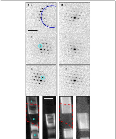
SPED data were acquired with precession angles of 0, 9 and 35 mrad from a GaAs nanowire oriented near to a [110] zone axis such that the twin boundary normal was approximately perpendicular to the incident beam direc-tion, as shown in Fig. 1. The bending of this nanowire is evident in the data acquired without precession (Fig. 1a) as at position iii the diffraction pattern is near the zone axis, whereas at position i a Laue circle is clearly visible. The radius of this Laue circle is ∼24 mrad , which
pro-vides an estimate of the bending angle across the field of view. When a precession angle of 35 mrad (i.e. larger than the bending angle) was used, all measured patterns appear close to zone axis (Fig. 1b) due to the reciprocal space integration resulting from the double conical rock-ing geometry. The effect of this integration is also seen in the contrast of the virtual dark-field image, which shows numerous bend contours without precession and less complex variation in intensity with precession. We surmise that precession leads to the data better approxi-mating the situation where there is a single diffraction pattern associated with each microstructural element, which here is essentially the two twinned crystal orien-tations and the vacuum surrounding the sample. The region of interest also contains a small portion of carbon support film, which is just visible in the virtual dark-field images as a small variation in intensity. The position of the carbon film has been indicated in the figure.
Fig. 1 SPED data from a GaAs nanowire and virtual dark-field images formed by plotting the intensity within the disks marked around {111}
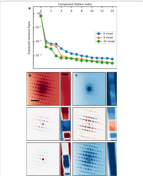
a log scale. This demonstrates that the use of precession reduces the number of components required to describe the data, consistent with the intuitive understanding of the effect of reciprocal space integration achieved using precession. The 4th component, significant in the 9 mrad data, arises because the top and bottom of the nanowire are sufficiently differently oriented, as a result of bend-ing, to be distinguished by the algorithm. We, therefore, continue our analysis focusing attention on data acquired with relatively large precession angles.
Component patterns and corresponding loading maps obtained by SVD and ICA analysis of 35 mrad SPED data are shown in Fig. 2b, c, respectively. In either analysis, each feature clearly describes some significant variation in the diffraction peak intensities, although it is worth noting that SVD requires two components to describe the two twins in the wire where ICA needs only one. Both descriptions of the data are mathematically sensible and physical insight can be obtained from the differences between diffraction patterns that are highlighted by neg-ative values in the SVD and ICA component patterns, but neither method produces patterns that can be directly associated with crystal structure. To make use of more conventional diffraction pattern analysis, we seek decom-position constraints that yield learned components which more closely resemble physical diffraction patterns. To this end, we apply NMF and fuzzy clustering.
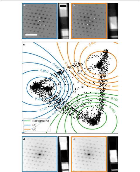
The data were decomposed to three component pat-terns using NMF, of which, by inspection, one corre-sponded to the background and two correcorre-sponded to the two twinned crystal orientations—the latter shown in Fig. 3a, b. The choice of three components was guided by the intrinsic dimensionality indicated by the SVD analysis and it was further verified that a plot of the NMF reconstruction error (Eq. 1) as a function of increasing number of components showed a similar regime change to the SVD scree plot (see “Availability of data and mate-rials” section at the end of the main text). In the NMF component patterns, white spots are visible, representing intensity lower than background level. We describe these as a pseudo-subtractive contribution of intensity from those locations.
In Fig. 3c, SVD loadings for the scan data are shown as a scatter plot, where the axes correspond to the SVD factors. Because the SVD and PCA factors are equiva-lent, this projection represents the maximum possible variation in the data, and so the maximum discrimina-tion. The loadings associated with each measured pat-tern are approximately distributed about a triangle in this space. Fuzzy clustering was applied to three SVD com-ponents, and the learned memberships are overlaid as contours. Three clusters describe the distribution of the loadings well, and the cluster centres correspond to the
background and the twinned crystals as shown in Fig. 3d, e. Both the NMF factors and c-means centers represent the same orientations, but the pseudo-subtractive arte-facts in the NMF factors are not present in the cluster centers.
The scatter plot in Fig. 3c also shows that two of the clusters comprise two smaller subclusters. Membership maps for these subclusters reveal that the splitting is due to the underlying carbon film with the subcluster nearer to the background cluster in each case corresponding to the region where the film is present. In the member-ship maps, there are bright lines along the boundaries between the nanowire and the vacuum, due to overlap between clusters.
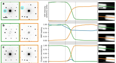
The unmixing of diffraction signals from overlapping crystals was investigated. SPED data with a precession angle of 18 mrad were acquired from a nanowire tilted away from the [110] zone axis by ∼30◦ , such that two
microstructural elements overlapped in projection. The overlap of the two crystals was assessed using virtual dark-field imaging, NMF loading maps, and fuzzy clus-tering membership maps (Fig. 4). The region in which the crystals overlap can be identified by all these meth-ods. The VDF result can be considered a reference and is obtained with minimal processing but requires man-ual specification of appropriate diffracting conditions for image formation. The NMF and fuzzy clustering approaches are semi-automatic. There is good agree-ment between the VDF images and NMF loading maps. The boundary appears slightly narrower in the cluster-ing membership map. The NMF loadcluster-ing correspondcluster-ing to the background component decreases along the pro-file, which may be related to the underlying carbon film, whilst the cluster membership for the background con-tains a spurious peak in the overlap region. Finally, the direct beam intensity is much lower in the NMF compo-nent patterns than in the true source signals. Our results indicate that either machine learning method is superior to conventional linear decomposition for the analysis of SPED datasets, but some unintuitive and potentially mis-leading features are present in the learning results.
Discussion
signal unmixing although we note that neither approach is well suited to situations where there are continuous changes in crystal structure. By contrast, SVD and ICA provide effective means of dimensionality reduction but the components are not readily interpreted using analo-gous methods to conventional electron diffraction analy-sis, owing to the presence of many negative values. The SVD and ICA results do nevertheless tend to highlight physically important differences in the diffraction signal across the region of interest. The massive data reduc-tion from many thousands of measured diffracreduc-tion pat-terns to a handful of learned component patpat-terns is very useful, as is the unmixing achieved. Artefacts in the learning results were however identified, particularly when applied to achieve signal unmixing, and these are explored further here.
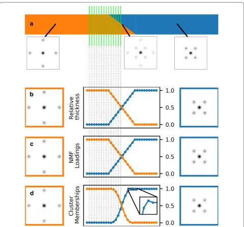
To illustrate artefacts resulting from learning meth-ods, model SPED datasets were constructed based on line scans across inclined boundaries in hypothetical bicrystals. Models (Figs. 5 and 6) were designed to high-light features of two-dimensional diffraction-like signals rather than to reflect the physics of diffraction. These were, therefore, constructed with the strength of the sig-nal directly proportiosig-nal to thickness of the hypothetical
crystal at each point, with no noise, and Gaussian peak profiles.
observations are consistent with the results reported in association with Fig. 4.
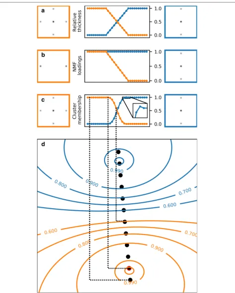
A common challenge for signal separation arises when the source signals contain coincident peaks from distinct microstructural elements, as would be the case in SPED data when crystallographic orientation rela-tionships exist between crystals. A model SPED data-set corresponding to this case was constructed and decomposed using NMF and fuzzy clustering (Fig. 6).
In this case, the NMF decomposition yields a tor containing all the common reflections and a fac-tor containing the reflections unique to only one end member. Whilst this is interpretable, it is not physi-cal, although it should be noted that this is an extreme example where there is no unique information in one of the source patterns. Nevertheless, it should be expected Fig. 5 Construction and decomposition of an idealised model SPED dataset system comprising non-overlapping two-dimensional signals. a
Fig. 6 Non-independent components. a Expected result for an artificial dataset with two ‘phases’ with overlapping peaks. b NMF decomposition. c
that the intensity of shared peaks is likely to be unreli-able in the learned factors and this was the case for the direct beam in learned component patterns shown in Fig. 4. As a result, components learned through NMF should not be analysed quantitatively3. The weighted average cluster centres resemble the true end members much more closely than the NMF components. The pure phases have a membership of around 99%, rather than 100%, due to the cluster centre being offset from the pure cluster by the mixed data, as shown in Fig. 6d. The observation that memberships extend across all the data (albeit sometimes with vanishingly small values) explains the rise in intensity of the background com-ponent in Fig. 4c in the interface region. Such interface regions do not evenly split their membership between their two true constituent clusters, meaning that some membership is attributed to the third cluster, causing a small increase in the membership locally. These issues
may potentially be addressed using extensions to the algorithm developed by Rousseeuw et al. [41] or using alternative geometric decompositions such as vertex component analysis [42].
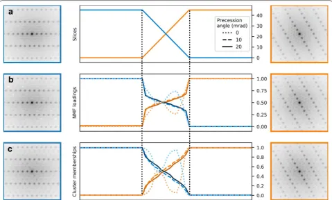
Precession was found empirically to improve machine learning decomposition as discussed above (Fig. 2), so long as the precession angle is large enough. This was attributed primarily to integration through bending of the nanowire. Precession may also result in a more monotonic variation of diffracted intensity with thick-ness [15] as a result of integration through the Bragg condition. It was, therefore, suggested that precession may improve the approximation that signals from two overlapping crystals may be considered to be combined linearly. To explore this, a multislice simulation of a line scan across a bi-crystal was performed and decomposed using both NMF and fuzzy clustering (Fig. 7). With-out precession, both the NMF loadings and the cluster memberships do not increase monotonically with thick-ness but rather vary significantly in a manner reminis-cent of diffracted intensity modulation with thickness due to dynamical scattering. Both the loading profile and the membership profile reach subsidiary minima Fig. 7 Unsupervised learning applied to SPED data simulated using dynamical multislice calculations a Original data with a 20 mrad precession angle. b NMF decomposition, in which the loadings have been re-scaled as in Fig. 5. The factors show pseudo-subtractive features, typical of NMF.
c Cluster analysis. The high proportion of data points from the boundary means there is information shared between the cluster centres. Without precession, neither method can reproduce the original data structure
3 This problem may be mitigated by enforcing a sum-to-one constraint on the
when the corresponding component is just thicker than half the thickness of the simulation, which corresponds to a thickness of approximately 100 nm and is consist-ent with the 220¯ extinction length for GaAs of 114 nm.
This suggests that the decomposition of the diffraction patterns is highly influenced by a few strong reflections; hence, the variation of the 220¯ reflections with
thick-ness is overwhelming the other structural information encoded in the patterns. The removal of this effect, an essential function of applying precession, is seen: with 10 or 20 mrad precession this intensity modulation is sup-pressed and the loading or membership maps obtained show a monotonic increase across the inclined boundary. The cluster centres again show intensity corresponding to the opposite end member due to the weighted averaging. Precession is, therefore, beneficial for the application of unsupervised learning algorithms both in reducing signal variations arising from bending, which is a common arte-fact of specimen preparation, and reducing the impact of dynamical effects on signal mixing.
Noise and background are both significant in determin-ing the performance of unsupervised learndetermin-ing algorithms. Extensive exploration of these parameters is beyond the scope of this work but we note that the various direct electron detectors that have recently been developed and that are likely to play a significant role in future SPED studies have very different noise properties. Therefore, understanding the optimal noise performance for unsu-pervised learning may become an important considera-tion. We also note that the pseudo-subtractive features evident in the NMF decomposition results of Fig. 3 may become more significant in this case and the robustness of fuzzy clustering to this may prove advantageous.
Conclusions
Unsupervised machine learning methods, particularly non-negative matrix factorisation and fuzzy clustering, have been demonstrated here to be capable of learning the sig-nificant microstructural features within SPED data. NMF may be considered a true linear unmixing whereas fuzzy clustering, when applied to learn representative patterns, is essentially an automated way of performing a weighted averaging with the weighting learned from the data. The former can struggle to separate coincident signals (includ-ing signal shared with a background or noise) whereas the latter implicitly leaves some mixing when a large fraction of measurements are mixed. In both cases, precession elec-tron diffraction patterns are more amenable to unsuper-vised learning than the static beam equivalents. This is due to the integration through the Bragg condition, resulting from rocking the beam, causing diffracted beam intensities
to vary more monotonically with thickness and the inte-gration through small orientation changes due to out of plane bending. This work has, therefore, demonstrated that unsupervised machine learning methods, when applied to SPED data, are capable of reducing the data to the most salient structural features and unmixing signals. The scope for machine learning to reveal nanoscale crystallography will expand rapidly in the coming years with the applica-tion of more advanced methods.
Abbreviations
BSS: blind source separation; FEGTEM: field-emission gun transmission electron microscope; ICA: independent component analysis; NNDSVD: non-negative double singular value decomposition; NMF: non-non-negative matrix factorisation; PED: precession electron diffraction; PCA: principal component analysis; SPED: scanning precession electron diffraction; STEM: scanning trans-mission electron microscopy; SVD: singular value decomposition; VBF: virtual bright field; VDF: virtual dark field.
Authors’ contributions
BHM, DNJ, ASE, and PAM proposed the investigation. DNJ, ASE, and ATJvH performed the SPED experiments, ASE provided the multislice simulations, and BHM implemented the c-means algorithm. The data analysis was under-taken by BHM and DNJ who also prepared the manuscript, with oversight and critical contributions from ASE, ATJvH, and PAM. All authors read and approved the final manuscript.
Author details
1 Department of Materials Science and Metallurgy, University of Cambridge, 27
Charles Babbage Road, Cambridge CB3 0FS, UK. 2 The School of Materials, The
University of Manchester, Oxford Road, Manchester M13 9PL, UK. 3
Depart-ment of Physics, Norwegian University of Science and Technology, Hogskoler-ing 5, 7491 Trondheim, Norway.
Acknowlegements
Prof. Weman and Fimland of IES at NTNU are acknowledged for supplying the nanowire samples.
Competing interests
The authors declare that they have no competing interests.
Availability of data and materials
Data used in this work has been made freely available to download at https :// doi.org/10.17863 /CAM.26432 .
The Python 3 code to perform the analysis has also been made available, at https ://doi.org/10.17863 /CAM.26444 .
Funding
The authors acknowledge financial support from: The Royal Society (Grant RG140453; UF130286); the Seventh Framework Programme of the European Commission: ESTEEM2, contract number 312483; the European Research Council under the European Union’s Seventh Framework Programme (FP7/2007-2013)/ERC grant agreement 291522-3DIMAGE; the University of Cambridge and the Cambridge NanoDTC; the EPSRC (Grant no. EP/ R008779/1).
Publisher’s Note
Springer Nature remains neutral with regard to jurisdictional claims in pub-lished maps and institutional affiliations.
References
1. Thomas, J.M., Leary, R.K., Eggeman, A.S., Midgley, P.A.: The rapidly chang-ing face of electron microscopy. Chem. Phys. Lett. 631, 103–113 (2015). https ://doi.org/10.1016/j.cplet t.2015.04.048
2. Murphy, K.P.: Machine Learning: A Probabilistic Perspective. Adaptive Computation and Machine Learning. MIT Press, Boston (2012) 3. de la Peña, F., Berger, M.H., Hochepied, J.F., Dynys, F., Stephan, O., Walls,
M.: Mapping titanium and tin oxide phases using EELS: an application of independent component analysis. Ultramicroscopy 111(2), 169–176 (2011). https ://doi.org/10.1016/J.ULTRA MIC.2010.10.001
4. Nicoletti, O., de la Peña, F., Leary, R.K., Holland, D.J., Ducati, C., Midgley, P.A.: Three-dimensional imaging of localized surface plasmon resonances of metal nanoparticles. Nature 502(7469), 80–84 (2013). https ://doi. org/10.1038/natur e1246 9
5. Rossouw, D., Burdet, P., de la Peña, F., Ducati, C., Knappett, B.R., Wheatley, A.E.H., Midgley, P.A.: Multicomponent signal unmixing from nanohet-erostructures: overcoming the traditional challenges of nanoscale X-ray analysis via machine learning. Nano Lett. 15(4), 2716–2720 (2015). https ://doi.org/10.1021/acs.nanol ett.5b004 49
6. Rossouw, D., Krakow, R., Saghi, Z., Yeoh, C.S., Burdet, P., Leary, R.K., de la Peña, F., Ducati, C., Rae, C.M., Midgley, P.A.: Blind source separation aided characterization of the γ ’ strengthening phase in an advanced nickel-based superalloy by spectroscopic 4D electron microscopy. Acta Mater. 107, 229–238 (2016). https ://doi.org/10.1016/j.actam at.2016.01.042 7. Rossouw, D., Knappett, B.R., Wheatley, A.E.H., Midgley, P.A.: A new method
for determining the composition of core-shell nanoparticles via dual-EDX+EELS spectrum imaging. Particle Particle Syst. Charact. 33(10), 749–755 (2016). https ://doi.org/10.1002/ppsc.20160 0096
8. Shiga, M., Tatsumi, K., Muto, S., Tsuda, K., Yamamoto, Y., Mori, T., Tanji, T.: Sparse modeling of EELS and EDX spectral imaging data by nonnega-tive matrix factorization. Ultramicroscopy 170, 43–59 (2016). https ://doi. org/10.1016/J.ULTRA MIC.2016.08.006
9. Eggeman, A.S., Krakow, R., Midgley, Pa: Scanning precession electron tomography for three-dimensional nanoscale orientation imaging and crystallographic analysis. Nat. Commun. 6, 7267 (2015). https ://doi. org/10.1038/ncomm s8267
10. Sunde, J.K., Marioara, C.D., Van Helvoort, A.T.J., Holmestad, R.: The evolu-tion of precipitate crystal structures in an Al-Mg-Si(-Cu) alloy studied by a combined HAADF-STEM and SPED approach. Mater. Charact. 142, 458–469 (2018). Mater . Chara ct10.1016/j.match ar.2018.05.031
11. Rauch, E.F., Veron, M.: Coupled microstructural observations and local tex-ture measurements with an automated crystallographic orientation map-ping tool attached to a TEM. Materialwissenschaft und Werkstofftechnik 36(10), 552–556 (2005). https ://doi.org/10.1002/mawe.20050 0923 12. Rauch, E.F., Portillo, J., Nicolopoulos, S., Bultreys, D., Rouvimov, S., Moeck, P.:
Automated nanocrystal orientation and phase mapping in the transmis-sion electron microscope on the basis of precestransmis-sion electron diffraction. Zeitschrift für Kristallographie 225(2–3), 103–109 (2010). https ://doi. org/10.1524/zkri.2010.1205
13. Vincent, R., Midgley, P.: Double conical beam-rocking system for measure-ment of integrated electron diffraction intensities. Ultramicroscopy 53(3), 271–282 (1994). https ://doi.org/10.1016/0304-3991(94)90039 -6 14. White, T., Eggeman, A., Midgley, P.: Is precession electron diffraction
kine-matical? Part I: “Phase-scrambling” multislice simulations. Ultramicroscopy 110(7), 763–770 (2010). https ://doi.org/10.1016/J.ULTRA MIC.2009.10.013 15. Eggeman, A.S., White, T.A., Midgley, P.A.: Is precession electron
diffrac-tion kinematical? Part II. A practical method to determine the optimum precession angle. Ultramicroscopy 110(7), 771–777 (2010). https ://doi. org/10.1016/j.ultra mic.2009.10.012
16. Sinkler, W., Marks, L.D.: Characteristics of precession electron diffraction intensities from dynamical simulations. Zeitschrift für Kristallographie 225(2–3), 47–55 (2010). https ://doi.org/10.1524/zkri.2010.1199 17. Rauch, E.F., Véron, M.: Virtual dark-field images reconstructed from
electron diffraction patterns. Eur. Phys. J. Appl. Phys. 66(1), 10,701 (2014). https ://doi.org/10.1051/epjap /20141 30556
18. Gammer, C., Burak Ozdol, V., Liebscher, C.H., Minor, A.M.: Diffraction con-trast imaging using virtual apertures. Ultramicroscopy 155, 1–10 (2015). https ://doi.org/10.1016/J.ULTRA MIC.2015.03.015
19. Rouviere, J.L., Béché, A., Martin, Y., Denneulin, T., Cooper, D.: Improved strain precision with high spatial resolution using nanobeam precession electron diffraction. Appl. Phys. Lett. 103(24), 241913 (2013). https ://doi. org/10.1063/1.48291 54
20. Moeck, P., Rouvimov, S., Rauch, E.F., Véron, M., Kirmse, H., Häusler, I., Neumann, W., Bultreys, D., Maniette, Y., Nicolopoulos, S.: High spatial resolution semi-automatic crystallite orientation and phase mapping of nanocrystals in transmission electron microscopes. Crys. Res. Technol. 46(6), 589–606 (2011). https ://doi.org/10.1002/crat.20100 0676 21. Kelly, A., Groves, G., Kidd, P.: Crystallography and Crystal Defects. Wiley,
Chichester (2000)
22. Munshi, A.M., Dheeraj, D.L., Fauske, V.T., Kim, D.C., Huh, J., Reinertsen, J.F., Ahtapodov, L., Lee, K.D., Heidari, B., van Helvoort, A.T.J., Fimland, B.O., Weman, H.: Position-controlled uniform GaAs nanowires on silicon using nanoimprint lithography. Nano Lett. 14(2), 960–966 (2014). https ://doi. org/10.1021/nl404 376m
23. Eggeman, A., London, A., Midgley, P.: Ultrafast electron diffraction pattern simulations using gpu technology. Applications to lattice vibrations. Ultramicroscopy 134, 44–47 (2013). https ://doi.org/10.1016/j.ultra mic.2013.05.013
24. Palatinus, L., Jacob, D., Cuvillier, P., Klementová, M., Sinkler, W., Marks, L.D.: IUCr: structure refinement from precession electron diffraction data. Acta Crystallogr. Sect. A Found. Crystallogr. 69(2), 171–188 (2013). https ://doi. org/10.1107/S0108 76731 20494 6X
25. Hoyer, P.O.: Non-negative matrix factorization with sparseness constraints. J. Mach. Learn. Res. 5, 1457–1469 (2004)
26. Jolliffe, I.: Principal component analysis. In: International Encyclopedia of Statistical Science, pp. 1094–1096. Springer , Berlin (2011)
27. Hyvärinen, A., Karhunen, J., Oja, E.: Independent Component Analysis. Wiley, New York (2001)
28. Lee, D.D., Seung, H.S.: Learning the parts of objects by non-negative matrix factorization. Nature 401(6755), 788–91 (1999). https ://doi. org/10.1038/44565
29. de la Pena, F., Ostasevicius, T., Tonaas Fauske, V., Burdet, P., Jokubauskas, P., Nord, M., Sarahan, M., Prestat, E., Johnstone, D.N., Taillon, J., Jan Caron, J., Furnival, T., MacArthur, K.E., Eljarrat, A., Mazzucco, S., Migunov, V., Aarholt, T., Walls, M., Winkler, F., Donval, G., Martineau, B., Garmannslund, A., Zago-nel, L.F., Iyengar, I.: Electron Microscopy (Big and Small) Data Analysis With the Open Source Software Package HyperSpy. Microsc. Microanal. 23(S1), 214–215 (2017). https ://doi.org/10.1017/S1431 92761 70017 51
30. Pedregosa, F., Varoquaux, G., Gramfort, A., Michel, V., Thirion, B., Grisel, O., Blondel, M., Prettenhofer, P., Weiss, R., Dubourg, V., Vanderplas, J., Passos, A., Cournapeau, D., Brucher, M., Perrot, M., Duchesnay, É.: Scikit-learn: machine learning in python. J. Mach. Learn. Res. 12(Oct), 2825–2830 (2011)
31. Shlens, J.: A tutorial on principal component analysis. CoRR (2014). arXiv :abs/1404.1100
32. Bishop, C.: Pattern Recognition and Machine Learning. Information Sci-ence and Statistics. Springer, New York (2006)
33. Boutsidis, C., Gallopoulos, E.: Svd based initialization: a head start for non-negative matrix factorization. Pattern Recogn. 41(4), 1350–1362 (2008). https ://doi.org/10.1016/j.patco g.2007.09.010
34. Everitt, B., Landau, S., Leese, M.: Clust. Anal. Wiley, Chichester (2009) 35. Bezdek, J.C., Ehrlich, R., Full, W.: FCM: the fuzzy c-means clustering
algorithm. Comput. Geosci. 10(2–3), 191–203 (1984). https ://doi. org/10.1016/0098-3004(84)90020 -7
36. Gustafson, D., Kessel, W.: Fuzzy clustering with a fuzzy covariance matrix. In: 1978 IEEE conference on decision and control including the 17th symposium on adaptive processes, pp. 761–766. IEEE, San Diego (1978). https ://doi.org/10.1109/CDC.1978.26802 8
37. Marimont, R.B., Shapiro, M.B.: Nearest neighbour searches and the curse of dimensionality. IMA J. Appl. Math. 24(1), 59–70 (1979). https ://doi. org/10.1093/imama t/24.1.59
38. Aggarwal, C.C., Hinneburg, A., Keim, D.A.: On the surprising behavior of distance metric in high-dimensional space (2002)
39. Rencher, A.: Methods of Multivariate Analysis. Wiley Series in Probability and Statistics. Wiley, Hoboken (2002)
unmixing: universal framework, domain examples, and a community-wide platform. Adv. Struct. Chem. Imaging 4(1), 6 (2018). https ://doi. org/10.1186/s4067 9-018-0055-8
41. Rousseeuw, P.J., Trauwaertb, E., Kaufman, L.: Fuzzy clustering with high contrast. J. Comput. Appl. Math. 0427(95), 8–9 (1995)