Chrono: a parallel multi-physics library for rigid-body, ﬂexible-body, and ﬂuid dynamics

(1)

Mech. Sci., 4, 49–64, 2013 www.mech-sci.net/4/49/2013/ doi:10.5194/ms-4-49-2013

©Author(s) 2013. CC Attribution 3.0 License.

Mechanical

Sciences

Open Access

Chrono: a parallel multi-physics library for rigid-body,

flexible-body, and fluid dynamics

H. Mazhar1_{, T. Heyn}1_{, A. Pazouki}1_{, D. Melanz}1_{, A. Seidl}1_{, A. Bartholomew}1_{, A. Tasora}2_{, and D. Negrut}1 1_{Simulation Based Engineering Lab, Department of Mechanical Engineering, University of Wisconsin,}

Madison, WI, 53706, USA

2_{Department of Industrial Engineering, University of Parma, V.G.Usberti 181}_/_{A, 43100, Parma, Italy}

Correspondence to: D. Negrut ([email protected])

Received: 16 November 2012 – Accepted: 26 January 2013 – Published: 12 February 2013

Abstract. The last decade witnessed a manifest shift in the microprocessor industry towards chip designs that promote parallel computing. Until recently the privilege of a select group of large research centers, Teraflop computing is becoming a commodity owing to inexpensive GPU cards and multi to many-core x86 processors. This paradigm shift towards large scale parallel computing has been leveraged inChrono, a freely available C++multi-physics simulation package.Chronois made up of a collection of loosely coupled components that facilitate different aspects of multi-physics modeling, simulation, and visualization. This contribution pro-vides an overview ofChrono::Engine,Chrono::Flex,Chrono::Fluid, andChrono::Render, which are modules that can capitalize on the processing power of hundreds of parallel processors. Problems that can be tackled inChronoinclude but are not limited to granular material dynamics, tangled large flexible structures with self contact, particulate flows, and tracked vehicle mobility. The paper presents an overview of each of these modules and illustrates through several examples the potential of this multi-physics library.

1 Introduction

Over the last decade there has been a manifest trend in the hardware industry to increase flop rates by increasing the number of cores available on a processor. To a very large extent, the tide that propelled sequential computing for sev-eral decades is subsiding. The frequency at which cores are operated today has at best plateaued; in many cases, it went down in an attempt to tame power dissipation and overheat-ing. Instruction level parallelism advances that ensured re-spectable gains through pipelining and out of order execu-tion have largely fulfilled their potential. The bright spot in this evolving hardware landscape has been the growing im-petus behind parallel computing hardware. If anything has held steady over the last four decades, it has been the pace at which transistors are packed per unit area in computer chips. This trend allows today chip designs that draw on 22 nm fea-ture length. Intel’s road map calls for 14 nm technology in 2014, 10 nm in 2016, 7 nm in 2018, and 5 nm in 2020. In other words, the number of transistors per unit area will

con-tinue to double every two years for the current decade. This will translate into immediate access to commodity chips that host multiple compute cores. Given the stagnation in proces-sor operating frequency, an ever growing gap between CPU speed and memory speed, and the waning of instruction level parallelism gains, it becomes apparent that the only way we can continue to enjoy reduced simulation times or ability to rely on refined models is to fall back on parallel comput-ing. There are two major directions in which parallel com-puting has evolved. The x86 architecture has defined a so-lution that evolved as a steady and predictable process in which the number of cores on a chip increased over time: AMD produces today 16 core chips, while Intel has 12 core processors. Leveraging these chips requires a low entry point that calls for programming against relatively mature libraries such as OpenMP, MPI, pthreads, cilk, TBB, etc. At mem-ory bandwidths of 75 GB s−1_{and flop rates of 0.3 TFlop s}−1_,

this has traditionally represented the conservative choice for entering the parallel computing arena. With the release of CUDA 1.0 in 2006, NVIDIA offered a second alternative

(2)

50 H. Mazhar et al.: Chrono: a parallel multi-physics library for rigid-body, flexible-body, and fluid dynamics

to leveraging parallel computing by programming the ubiq-uitous video cards available on millions of desktops world-wide. This path to parallel computing is less conventional as it requires one to get familiar with the hardware layout and memory hierarchy associated with GPUs. Today, an Nvidia GPU has close to seven billion transistors. Priced at about $6000, an Nvidia Kepler K20x delivers a memory bandwidth of 250 GB s−1_{and 1.3 TFlop s}−1_{by virtue of using more than}

2800 Scalar Processors. It is used side by side with a regular CPU processor, which means that heterogeneous computing, on the CPU and GPU, can lead to substantial speed gains. In this framework, the GPU plays the role of an accelerator by boosting the floating point performance of the CPU. A sim-ilar setup is offered now by Intel; i.e., CPU plus accelerator, owing to its recent release of the Knights Corner architec-ture. A Knights Corner chip has about 60 cores, can deliver up to 320 GB s−1 _{and 1 TFlop s}−1_{, and uses the x86}

instruc-tion set architecture, which translates into an easier adopinstruc-tion path provided one is familiar with OpenMP or MPI.

It becomes apparent that in the immediate future, any in-crease in simulation speed or model complexity in Compu-tational Science will be fueled by parallel computing. This paper outlines an ongoing effort in the area of computational mutlibody dynamics that is motivated by this belief. It starts with a description of a core simulation engine that aims at simulation of many-body dynamics problems with friction and contact.Chrono::Engine handles both rigid and flexible bodies and draws on MPI and/or GPU computing. It then discussesChrono::Fluid, a GPU parallel simulation tool that aims at fluid-solid interaction problems, which is singled out as an application area that has been largely ignored until re-cently due to an excessive computational burden incurred by the simulation of systems of practical relevance. Finally, the papers outlines a rendering pipeline that is used for postpro-cessing of big data.Chrono::Render is capable of using 320 cores and is built around Pixar’s RenderMan. All these com-ponents combine to produceChrono, a multi-physics simu-lation environment that is designed to take advantage of com-modity parallel computing made available by many-core and GPU architectures.

2 Chrono::Engine

TheChrono::Engine software is a general-purpose simulator for three dimensional multi-body problems (Tasora and An-itescu, 2011). Specifically, the code is designed to support the simulation of very large systems such as those encountered in granular dynamics, where the number of interacting elements can be in the millions. Target applications include tracked vehicles operating on granular terrain (Heyn, 2009) or the Mars Rover operating on discrete granular soil. In these ap-plications, it is desirable to model the granular terrain as a collection of many thousands or millions of discrete bodies interacting through contact, impact, and friction. Note that

such systems also include mechanisms composed of rigid bodies and mechanical joints. These challenges require an ef-ficient and robust simulation tool, which has been developed in theChronosimulation package.Chrono::Engine was ini-tially developed leveraging the Differential Variational In-equality (DVI) formulation as an efficient method to deal with problems that encompass many frictional contacts – a typical bottleneck for other types of formulations (Anitescu and Tasora, 2010; Tasora and Anitescu, 2010). This approach enforces non-penetration between rigid bodies through con-straints, leading to a cone-constrained quadratic optimiza-tion problem which must be solved at each time step (Ne-grut et al., 2012).Chrono::Engine has since been extended to support the Discrete Element Method (DEM) formula-tion for handling the fricformula-tional contacts present in granu-lar dynamics problems (Cundall, 1971; Cundall and Strack, 1979). This formulation computes contact forces by penaliz-ing small interpenetrations of collidpenaliz-ing rigid bodies. Various contact force models can be used depending on the applica-tion (Mindlin and Deresiewicz, 1953; Kruggel-Emden et al., 2007).

The remainder of this section describes the features of

Chrono::Engine, starting with the structure of the code. Next, several sub-sections describe the use of GPU computing in the collision detection task, the use of MPI for distributed so-lution of large systems, and validation work which has been done to assess the accuracy of the simulation tool.

2.1 Code structure of Chrono::Engine

The core ofChrono::Engine is built around the concept of middleware, namely a layer of classes and functions that can be used by third-party developers to create complex mechan-ical simulation software with little effort (Tasora et al., 2007). Because of this, graphical user interfaces and end-user tools are not the main focus of theChrono::Engine core project; it is assumed that programs with graphical interfaces are built on top of such middleware, or should be considered as addi-tional, or opaddi-tional, modules.

Given the complexity of the project, approaching half a million lines of code, the software is organized in classes and namespaces as recommended by the Object Oriented Programming paradigm, targeting modularity, en-capsulation, reusability and polymorphism. The libraries of

Chrono::Engine are thread safe, fully re-entrant, and include more than six hundred C++ classes. Objects from these classes can be instantiated and used to define models and simulations that run in third party software, for instance ve-hicle simulators, CAD tools, virtual reality applications, or robot simulators.

Chrono::Engine is completely platform-independent, hence libraries are available for Windows, Linux and Mac OSx, for both 32 bit and 64 bit versions. Moreover, we fol-lowed a modular approach, splitting the libraries in mod-ules that can be dynamically loaded only if necessary, thus

(3)

H. Mazhar et al.: Chrono: a parallel multi-physics library for rigid-body, flexible-body, and fluid dynamics 51

minimizing issues of dependency from other libraries and reducing memory footprint. For instance, we developed li-braries for MATLAB interoperability, for real-time visualiza-tion through OpenGL, for interfacing with post-processing tools, etc. (see Fig. 1).

Classes and objects have been tested and profiled for fast execution, in order to achieve real-time performance when possible. Modern programming techniques have been adopted, like metaprogramming, class templating, class fac-tories, memory leak trackers and persistent-transient data mapping. C++operator overloading has been used to provide a compact algebra to manage quaternions, static and moving coordinate systems, and OS-agnostic classes are used for log-ging, streaming/checkpointing and exception handling.

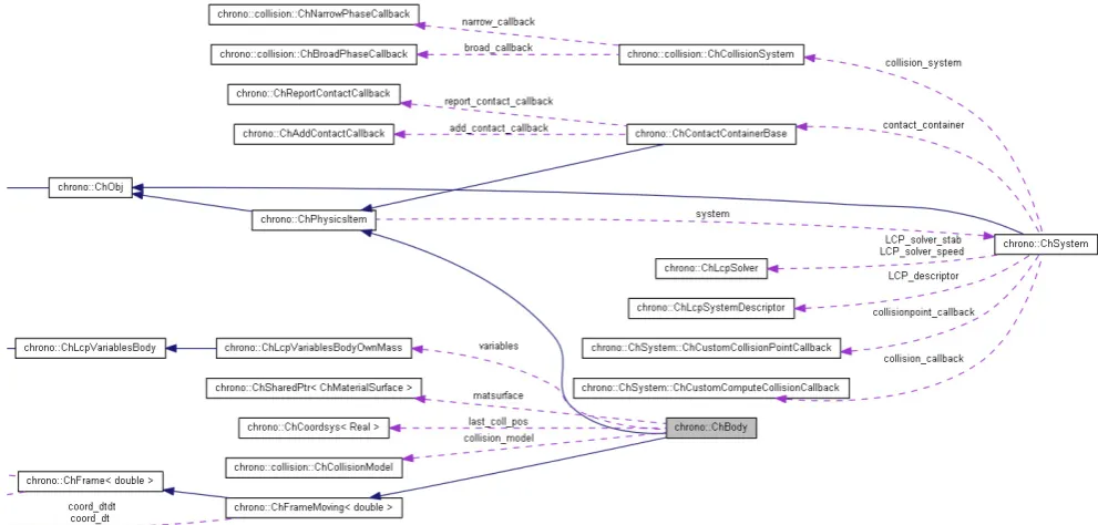
We embraced an intense object-oriented approach, there-fore most C++ objects that define parts of the multi-body model are inherited from a base class called

ChPhysicsItem, which defines the essential interfaces for all items that have some degrees of freedom. For example, specialized classes that inherit theChPhysicsItem are the

ChBodyclass, which is used for 3-D rigid bodies as shown in Fig. 2,ChShaft, which is used for 1-D concentrated pa-rameter models of power trains,ChLinkLockRevolutethat is a joint between rigid bodies, and so on. A set of more than thirty mechanical constraints are part of this class hierarchy. Furthermore, the architecture is open to further definition of new specialized classes for user-customized parts and joints. An object ofChSystemclass stores a list of all moving parts and performs the simulation.

EachChPhysicsItem-inheriting class can encapsulate a variable number of ChLcpVariableobjects and/or a vari-able number ofChLcpConstraintobjects, that are fed to the solver for Cone Complementarity Problems (CCP) at each time step of the DVI integration; this helps the devel-opment of black-box CCP solvers that are independent from the data structures of the physical layer. Also, these data structures represent the sparse data for the model descrip-tion, which is completely matrix- and vector-free for the sake of a small memory footprint and fast linear algebra. Specifi-cally, tthe system matrices for mass, Jacobians, etc. are never explicitly assembled. The objects of most of the above men-tioned classes are managed by smart (shared) pointers with automatic deletion.

This relieves the programmer from the burden of taking care of object’s lifetime, given that the relationships between objects can be quite complex as illustrated in Fig. 3. A large portion of the C++classes are available also as Python mod-ules; this enables the use of most simulation features in a scripted environment. Since novice users are more comfort-able with Python than with C++, the Python interface proved to be optimal for teaching purposes. The Python interface was produced using the SWIG utility, a process that auto-matically generates the code for the Python wrapper.

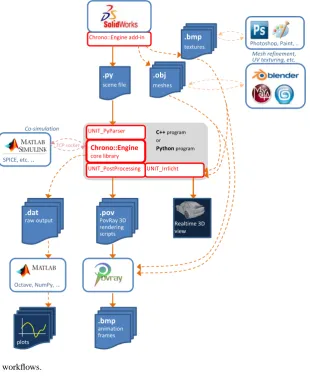
The software architecture has been designed to accommo-date an expandable system for handling assets (meshes,

tex-tures, CAD models), with multiple paths from pre-processing to post-processing. To this end, we also provide a C# add-in for a parametric 3-D CAD package (SolidWorks) that can be used to export models intoChrono::Engine without pro-gramming efforts (see Fig. 4).

2.2 Collision detection in Chrono::Engine

This section describes the collision detection algorithm de-signed and implemented for the Chrono::Engine package. Recall that problems of interest are focused on granular dy-namics, such as sand flowing inside an hourglass, a rover running over sandy terrain, an excavator/frontloader dig-ging/loading granular material, etc. In this context, the col-lision detection task is performed on a rather small collec-tion of rigid and/or deformable bodies of complex geome-try (hourglass wall, wheel, track shoe, excavator blade, dip-per), and a very large number of bodies (millions to billions) that make up the granular material. On this scale, the colli-sion detection task, particularly when dealing with the gran-ular material, fits perfectly the Single Instruction Multiple Data (SIMD) computation paradigm. Specifically, the same sequence of instructions needs to be applied to every indi-vidual body and/or contact in the granular material. There-fore, a collision detection algorithm capable of leveraging the SIMD computational power of commodity Graphics Pro-cessing Units (GPUs) was developed and implemented to re-move collision detection as the bottleneck in large granular dynamics simulations.

The parallel collision detection algorithm is separated into two phases, broadphase, and narrowphase. The broadphase algorithm quickly determines a list of potential contact pairs while the narrowphase algorithm determines actual contact information. A brief outline of the parallel collision detection algorithm is presented below, for more details see (Mazhar et al., 2011; Pazouki et al., 2012, 2010).

2.2.1 Broad-Phase algorithm

The Broad-Phase algorithm is used to compute whether two bodies might be in contact at a given time. The purpose of the broad-phase algorithm is not to find actual contact infor-mation, but rather to determine if a contact could potentially occur based on the Axis Aligned Bounding Boxes of the bod-ies involved.

An Axis Aligned Bounding Box (AABB) is a special case of a bounding box that is always aligned to the global refer-ence frame, simplifying collision detection as the bounding box cannot rotate. Because of this, the volume enclosed by the bounding box will always be equal to or greater than the volume of the shape it encloses. AABB generation is simple and can be easily paralellized on a per object basis. See Fig. 5 for an example of AABB computation for a cylinder in 3-D space.

(4)

Mazhar et al.:

Chrono

: A Parallel Multi-Physics Library for Rigid-Body, Flexible-Body, and Fluid Dynamics

3

OpenGL

unit_IRRLICHT Chrono Engine

unit_POSTPROCESS unit_MATLAB

MATLAB

Operating System Irrlicht

unit_OPENGL

unit_CASCADE unit_PYTHON

Python v3

OpenCASCADE unit_MPI unit_GPU

CUDA MPICH2

Chrono libraries

Example C++ program 'A' Example C++ program 'B' Example Python program

Examples of use

External dependencies

Figure 1

: UML graph of dependencies between module libraries.

tion through OpenGL, for interfacing with post-processing

tools, etc. (see Figure 1).

Classes and objects have been tested and profiled for fast

ex-ecution, in order to achieve real-time performance when

pos-sible. Modern programming techniques have been adopted,

like metaprogramming, class templating, class factories,

memory leak trackers and persistent-transient data mapping.

C

++

operator overloading has been used to provide a

com-pact algebra to manage quaternions, static and moving

coor-dinate systems, and OS-agnostic classes are used for logging,

streaming

/

checkpointing and exception handling.

We embraced an intense object-oriented approach, therefore

most C

++

objects that define parts of the multi-body model

are inherited from a base class called

ChPhysicsItem

,

which defines the essential interfaces for all items that have

some degrees of freedom. For example, specialized classes

that inherit the

ChPhysicsItem

are the

ChBody

class, which

is used for 3D rigid bodies as shown in Fig.2,

ChShaft

,

which is used for 1D concentrated parameter models of

power trains,

ChLinkLockRevolute

that is a joint between

rigid bodies, and so on. A set of more than thirty

mechani-cal constraints are part of this class hierarchy. Furthermore,

the architecture is open to further definition of new

special-ized classes for user-customspecial-ized parts and joints. An object

of

ChSystem

class stores a list of all moving parts and

per-forms the simulation.

Each

ChPhysicsItem

-inheriting class can encapsulate a

variable number of

ChLcpVariable

objects and

/

or a

vari-able number of

ChLcpConstraint

objects, that are fed to

the solver for Cone Complementarity Problems (CCP) at

each time step of the DVI integration; this helps the

devel-opment of black-box CCP solvers that are independent from

the data structures of the physical layer. Also, these data

structures represent the sparse data for the model description,

which is completely matrix- and vector-free for the sake of a

small memory footprint and fast linear algebra. Specifically,

Figure 2

: Class ineritance diagram for objects of

ChBody

type.

tthe system matrices for mass, Jacobians, etc. are never

ex-plicitly assembled. The objects of most of the above

men-tioned classes are managed by smart (shared) pointers with

automatic deletion.

This relieves the programmer from the burden of taking care

of object’s lifetime, given that the relationships between

ob-jects can be quite complex as illustrated in Fig.3. A large

por-tion of the C

++

classes are available also as Python modules;

this enables the use of most simulation features in a scripted

environment. Since novice users are more comfortable with

Python than with C

++

, the Python interface proved to be

op-timal for teaching purposes. The Python interface was

pro-duced using the SWIG utility, a process that automatically

generates the code for the Python wrapper.

The software architecture has been designed to accommodate

an expandable system for handling assets (meshes, textures,

CAD models), with multiple paths from pre-processing to

post-processing. To this end, we also provide a C# add-in for

a parametric 3D CAD package (SolidWorks) that can be used

to export models into

Chrono

::Engine without programming

e

ff

orts (see Fig.4).

2.2

Collision Detection in

Chrono

::Engine

This section describes the collision detection algorithm

de-signed and implemented for the

Chrono

::Engine package.

Recall that problems of interest are focused on granular

dy-namics, such as sand flowing inside an hourglass, a rover

running over sandy terrain, an excavator

/

frontloader

dig-ging

/

loading granular material, etc. In this context, the

col-lision detection task is performed on a rather small

collec-tion of rigid and

/

or deformable bodies of complex

geome-try (hourglass wall, wheel, track shoe, excavator blade,

dip-per), and a very large number of bodies (millions to billions)

that make up the granular material. On this scale, the

colli-sion detection task, particularly when dealing with the

gran-Figure 1.UML graph of dependencies between module libraries.

Figure 2.Class ineritance diagram for objects ofChBodytype.

2.2.2 Spatial Subdivision algorithm

A high-level overview of the GPU-based collision detection is as follows. The collision detection process starts by identi-fying the intersections between AABBs and bins (see Fig. 6 for a visual representation of a bin). The AABB-bin pairs are subsequently sorted by bin id. Next, each bin’s starting in-dex is determined so that the bins’ AABBs can be traversed sequentially. All AABBs touching a bin are subsequently checked against each other for collisions.

2.2.3 Narrow-Phase algorithm

Once potential contacts have been determined from the broad-phase collision detection stage, the Narrow-Phase al-gorithm needs to process each possible contact and determine if it actually occurs. To this end an algorithm capable of de-termining contacts between convex geometries was imple-mented on the GPU. This algorithm, called “XenoCollide” (Snethen, 2007), is based upon Minkowski Portal Refinement (MPR) (Snethen, 2008).

(5)

4 Mazhar et al.:Chrono: A Parallel Multi-Physics Library for Rigid-Body, Flexible-Body, and Fluid Dynamics

Figure 3: Collaboration graph between classes: example forChBodyandChSystem.

ular material, fits perfectly the Single Instruction Multiple Data (SIMD) computation paradigm. Specifically, the same sequence of instructions needs to be applied to every indi-vidual body and/or contact in the granular material. There-fore, a collision detection algorithm capable of leveraging the SIMD computational power of commodity Graphics Pro-cessing Units (GPUs) was developed and implemented to re-move collision detection as the bottleneck in large granular dynamics simulations.

The parallel collision detection algorithm is separated into two phases, broadphase, and narrowphase. The broadphase algorithm quickly determines a list of potential contact pairs while the narrowphase algorithm determines actual contact information. A brief outline of the parallel collision detection algorithm is presented below, for more details see (Mazhar et al., 2011; Pazouki et al., 2012, 2010).

2.2.1 Broad-Phase Algorithm

The Broad-Phase algorithm is used to compute whether two bodies might be in contact at a given time. The purpose of the broad-phase algorithm is not to find actual contact infor-mation, but rather to determine if a contact could potentially occur based on the Axis Aligned Bounding Boxes of the bod-ies involved.

An Axis Aligned Bounding Box (AABB) is a special case of a bounding box that is always aligned to the global refer-ence frame, simplifying collision detection as the bounding box cannot rotate. Because of this, the volume enclosed by the bounding box will always be equal to or greater than the

Chrono::Engine

core library UNIT_PyParser

UNIT_PostProcessing UNIT_Irrlicht

C++program or

Pythonprogram

.py

scene file

.obj

meshes

.pov

PovRay 3D rendering scripts

.bmp

animation frames

.dat

raw output

Octave, NumPy, ..

Chrono::Engine add-in

plots

SPICE, etc. .. Co-simulation

TCP socket

Mesh refinement, UV texturing, etc.

Realtime 3D view

Photoshop, Paint, ..

.bmp

textures

Figure 4: Network of asset workflows.

volume of the shape it encloses. AABB generation is sim-ple and can be easily paralellized on a per object basis. See Fig. 5 for an example of AABB computation for a cylinder in 3D space.

Mech. Sci. www.mech-sci.net

Figure 3.Collaboration graph between classes: example forChBodyandChSystem.

2.3 Using MPI for distributed Chrono

Chronohas been further extended to allow the use of CPU parallelism for certain problems. To efficiently simulate large systems, a domain decomposition approach has been devel-oped to allow the use of many-core compute clusters. In this approach, we divide the simulation domain into a number of sub-domains in a lattice structure. Each sub-domain manages the simulation of all bodies contained therein. Note that bod-ies may span the boundary between adjacent sub-domains. In this case, the body is considered shared and its dynamics may be influenced by the participating sub-domains. The im-plementation leverages the MPI standard (Gropp et al., 1999) to implement the necessary communication and synchroniza-tion between sub-domains.

This approach enables the simulation of large systems in two ways. First, it relies on the power of parallel comput-ing since one computer core can be assigned to each MPI process (and therefore to each sub-domain). These processes can execute in parallel, constrained only by the required com-munication and synchronization. Second, it allows access to the larger memory pool available on distributed memory ar-chitectures. Whereas a single node or GPU card may have about 6 GB of memory, a distributed memory cluster may have on the order of 1 TB of memory, enabling the simula-tion of vastly larger problems.

Note that the domain decomposition approach currently uses the discrete element method to resolve friction and con-tact forces between elements in the system. The approach also supports constraints between bodies in the simulation by considering an assembly of constrained rigid bodies as a

unit which must always be kept together. Therefore, if any body in a chain of constrained bodies is contained in a given sub-domain, all bodies in the chain are considered by that sub-domain and used to correctly solve the constraint equa-tions.

2.3.1 Sub-division and set-up

A pre-processing step is used to discretize the simulation domain into a specified number of sub-domains, set up the communication conduits between processes, and initialize the sub-domains as appropriate. The sub-division is based on a cubic lattice with support for arbitrary sized divisions. The sub-domain boundaries are aligned with the global carte-sian coordinate system, and their locations are user-specified. Separate MPI processes are mapped to each sub-domain. Note that at this time, the sub-division is static and does not change during the simulation. Therefore, the user should be careful to set up the discretization to maintain the best possi-ble load balancing.

In terms of communication, each sub-domain in the grid can communicate with all other sub-domains. These commu-nication pathways are set up and initialized during the pre-processing step and persist throughout the simulation.

Note that this implementation relies heavily on inheri-tance and the class-based structure of Chrono. For exam-ple, ChSystem is extended to ChSystemMPI by including the code to perform communication and synchronize the sub-domains.

(6)

4

Mazhar et al.:

Chrono

Figure 3

: Collaboration graph between classes: example for

ChBody

and

ChSystem

.

ular material, fits perfectly the Single Instruction Multiple

Data (SIMD) computation paradigm. Specifically, the same

sequence of instructions needs to be applied to every

indi-vidual body and

/

or contact in the granular material.

There-fore, a collision detection algorithm capable of leveraging

the SIMD computational power of commodity Graphics

Pro-cessing Units (GPUs) was developed and implemented to

re-move collision detection as the bottleneck in large granular

dynamics simulations.

The parallel collision detection algorithm is separated into

two phases, broadphase, and narrowphase. The broadphase

algorithm quickly determines a list of potential contact pairs

while the narrowphase algorithm determines actual contact

information. A brief outline of the parallel collision detection

algorithm is presented below, for more details see (Mazhar

et al., 2011; Pazouki et al., 2012, 2010).

2.2.1

Broad-Phase Algorithm

The Broad-Phase algorithm is used to compute whether two

bodies might be in contact at a given time. The purpose of

the broad-phase algorithm is not to find actual contact

infor-mation, but rather to determine if a contact could potentially

occur based on the Axis Aligned Bounding Boxes of the

bod-ies involved.

An Axis Aligned Bounding Box (AABB) is a special case

of a bounding box that is always aligned to the global

refer-ence frame, simplifying collision detection as the bounding

box cannot rotate. Because of this, the volume enclosed by

the bounding box will always be equal to or greater than the

Chrono::Engine

core library UNIT_PyParser

UNIT_PostProcessing UNIT_Irrlicht

C++program or

Pythonprogram

.py

scene file

.obj

meshes

.pov

PovRay 3D rendering scripts

.bmp

animation frames

.dat

raw output

Octave, NumPy, ..

Chrono::Engine add-in

plots SPICE, etc. ..

Co-simulation

TCP socket

Mesh refinement, UV texturing, etc.

Realtime 3D view

Photoshop, Paint, .. .bmp

textures

Figure 4

: Network of asset workflows.

volume of the shape it encloses. AABB generation is

sim-ple and can be easily paralellized on a per object basis. See

Fig. 5 for an example of AABB computation for a cylinder

in 3D space.

Mech. Sci.

www.mech-sci.net

Figure 4.Network of asset workflows.

Figure 5.Example of AABB generation for 3-D cylinder.

2.3.2 Simulation and communication

Each sub-domain is now represented by aChSystemMPI ob-ject and an associated MPI process. For example, assume a simulation is discretized into a set S of m sub-domains. In this case, let S ={A,B,C,D} and m=4, and map an MPI

Mazhar et al.:

Chrono

5

Minimum Point

Maximum Point

Figure 5

: Example of AABB generation for 3D cylinder.

3-Dimensional Grid

Bin

Figure 6

: Example of 3D space divided into bins.

2.2.2

Spatial Subdivision Algorithm

A high-level overview of the GPU-based collision detection

is as follows. The collision detection process starts by

identi-fying the intersections between AABBs and bins (see Fig. 6

for a visual representation of a bin). The AABB-bin pairs are

subsequently sorted by bin id. Next, each bin’s starting

in-dex is determined so that the bins’ AABBs can be traversed

sequentially. All AABBs touching a bin are subsequently

checked against each other for collisions.

2.2.3

Narrow-Phase Algorithm

Once potential contacts have been determined from the

broad-phase collision detection stage, the Narrow-Phase

al-gorithm needs to process each possible contact and

deter-mine if it actually occurs. To this end an algorithm

capa-ble of determining contacts between convex geometries was

implemented on the GPU. This algorithm, called

“XenoCol-lide” (Snethen, 2007), is based upon Minkowski Portal

Re-finement (MPR) (Snethen, 2008).

2.3

Using MPI for distributed

Chrono

has been further extended to allow the use of CPU

parallelism for certain problems. To e

ffi

ciently simulate large

systems, a domain decomposition approach has been

devel-oped to allow the use of many-core compute clusters. In this

approach, we divide the simulation domain into a number of

sub-domains in a lattice structure. Each sub-domain manages

the simulation of all bodies contained therein. Note that

bod-ies may span the boundary between adjacent sub-domains.

In this case, the body is considered shared and its dynamics

may be influenced by the participating sub-domains. The

im-plementation leverages the MPI standard (Gropp et al., 1999)

to implement the necessary communication and

synchroniza-tion between sub-domains.

This approach enables the simulation of large systems in two

ways. First, it relies on the power of parallel computing since

one computer core can be assigned to each MPI process (and

therefore to each sub-domain). These processes can execute

in parallel, constrained only by the required communication

and synchronization. Second, it allows access to the larger

memory pool available on distributed memory architectures.

Whereas a single node or GPU card may have about 6 GB of

memory, a distributed memory cluster may have on the order

of 1TB of memory, enabling the simulation of vastly larger

problems.

Note that the domain decomposition approach currently uses

the discrete element method to resolve friction and contact

forces between elements in the system. The approach also

supports constraints between bodies in the simulation by

considering an assembly of constrained rigid bodies as a unit

which must always be kept together. Therefore, if any body

in a chain of constrained bodies is contained in a given

domain, all bodies in the chain are considered by that

sub-domain and used to correctly solve the constraint equations.

2.3.1

Sub-division and Set-up

A pre-processing step is used to discretize the simulation

domain into a specified number of sub-domains, set up the

communication conduits between processes, and initialize

the sub-domains as appropriate. The sub-division is based

on a cubic lattice with support for arbitrary sized divisions.

The sub-domain boundaries are aligned with the global

carte-sian coordinate system, and their locations are user-specified.

Separate MPI processes are mapped to each sub-domain.

Note that at this time, the sub-division is static and does not

change during the simulation. Therefore, the user should be

careful to set up the discretization to maintain the best

possi-ble load balancing.

In terms of communication, each sub-domain in the grid can

communicate with all other sub-domains. These

commu-nication pathways are set up and initialized during the

pre-processing step and persist throughout the simulation.

Note that this implementation relies heavily on inheritance

and the class-based structure of

Chrono

.

For example,

ChSystem

is extended to

ChSystemMPI

by including the

code to perform communication and synchronize the

sub-domains.

Figure 6.Example of 3-D space divided into bins.

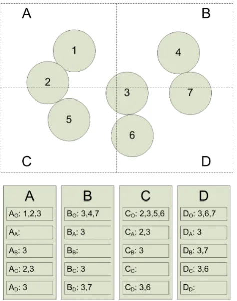
rank to each sub-domain so that A is mapped to MPI rank 0, B→1, C→2, and D→3. Each sub-domain maintains at all times m+1 lists of objects. The first list contains all objects which are even partially contained in the associated sub-domain. These are the objects which must be considered

(7)

6

Mazhar et al.:

Chrono

2.3.2 Simulation and Communication

Each sub-domain is now represented by a

ChSystemMPI

ob-ject and an associated MPI process. For example, assume

a simulation is discretized into a set

S

of

m

sub-domains.

In this case, let

S

=

{

A

,

B

,

C

,

D

}

and

m

=

4, and map an MPI

rank to each sub-domain so that

A

is mapped to MPI rank

0,

B

→

1,

C

→

2, and

D

→

3. Each sub-domain maintains

at all times

m

+

1 lists of objects. The first list contains all

objects which are even partially contained in the associated

sub-domain. These are the objects which must be considered

when computing contact forces, for example. The next

m

lists contain bodies which are shared with other sub-domains.

In our example, sub-domain

B

maintains the lists

B

O

,

B

A

,

B

,

B

C

, and

B

D

.

B

O

is the list of all objects that intersect (touch)

sub-domain

B

, while

B

A

is the list of objects which are in

sub-domain

A

and

B

. Note that sub-domain

A

has a list

A

B

which should contain the same objects as

B

A

. Further, list

B

is not used but is created for the sake of generality. All

lists are maintained in order sorted by object ID number (see

Fig.7).

Figure 7: (TOP) Sample 2D simulation domain with four

sub-domains and seven objects. (BOTTOM) Corresponding object lists for each sub-domain.

The domains are now ready for time-stepping. Each

sub-domain

X

performs collision detection among all objects in

list

X

O

and computes the associated collision forces based on

the DEM force model. Then, sub-domain

X

computes the

net force on each object in list

X

O

, taking into account the

contact forces, gravitational forces, and applied forces.

Next, mid-step communication occurs.

Sub-domain

X

should send to each sub-domain

Y

the net force on each body

in list

X

Y

. Similarly,

X

should receive from each

Y

the net

force on each body in list

X

Y

. Finally,

X

should compute the

total force on each body in list

X

O

. Note that

X

may receive

force contributions for a given body from any or all of the

other sub-domains in the system.

At this point, each sub-domain

X

has the true net force on

each body in its list

X

O

. Each sub-domain can advance the

state of its bodies in time by one time step by computing the

new accelerations, velocities, and positions of all objects in

the sub-domain given their mass

/

inertia properties and the set

of applied forces. We perform an end-of-step communication

to synchronize object states among domains. All

sub-domains which share a given body should compute its new

state identically, but due to the potential for round-o

ff

error

we synchronize the state from the master sub-domain (where

the center-of-mass is located) to all others. The final stage

is to process the

m

+

1 lists in each sub-domain, as objects

may enter or leave a given sub-domain or be shared between

a di

ff

erent set of sub-domains, necessitating updates of the

contents of the lists.

2.3.3 Example Simulation

In this example we simulate a Mars Rover type wheeled

ve-hicle operating on granular terrain. The veve-hicle is composed

of a chassis and six wheels connected via revolute joints.

The wheels are driven with a constant angular velocity of

π

rad

/

sec. The granular terrain is composed of 2,016,000

spherical particles. The simulation is divided into 64

sub-domains and uses a time step of 10

−5

sec. This small time

step is necessary due to the use of the DEM approach to

com-pute contact forces - a sti

ff

force model is used to achieve

small normal interpenetration, requiring a small step size to

maintain stability. A snapshot from the simulation can be

seen in Fig.8. In the figure, note that the wheels of the rover

are checkered blue and white. This signifies that the master

copy of the rover assembly is in the blue sub-domain and the

rover spans into adjacent sub-domains. In Fig. 8, the rover

has settled into the granular terrain and is starting to move

forward. The rear wheels displace more granular material

than the front wheels because the center of mass of the rover

is closer to the rear of the vehicle.

2.4 Validation and Demonstration of Technology

This section describes a validation e

ff

ort in which

experi-mental results were compared to simulation results obtained

from

Chrono

::Engine. To this end, a test rig was designed

Mech. Sci.

www.mech-sci.net

Figure 7. (Top) Sample 2-D simulation domain with four sub-domains and seven objects. (Bottom) Corresponding object lists for each sub-domain.

when computing contact forces, for example. The next m lists contain bodies which are shared with other sub-domains.

In our example, sub-domain B maintains the lists BO, BA,

BB, BC, and BD. BO is the list of all objects that intersect

(touch) sub-domain B, while BA is the list of objects which

are in sub-domain A and B. Note that sub-domain A has a list

ABwhich should contain the same objects as BA. Further, list

BB is not used but is created for the sake of generality. All

lists are maintained in order sorted by object ID number (see Fig. 7).

The sub-domains are now ready for time-stepping. Each sub-domain X performs collision detection among all objects in list XOand computes the associated collision forces based

on the DEM force model. Then, sub-domain X computes the net force on each object in list XO, taking into account the

contact forces, gravitational forces, and applied forces. Next, mid-step communication occurs. Sub-domain X should send to each sub-domain Y the net force on each body in list XY. Similarly, X should receive from each Y the net

force on each body in list XY. Finally, X should compute the

total force on each body in list XO. Note that X may receive

force contributions for a given body from any or all of the other sub-domains in the system.

At this point, each sub-domain X has the true net force on each body in its list XO. Each sub-domain can advance

the state of its bodies in time by one time step by computing the new accelerations, velocities, and positions of all objects in the sub-domain given their mass/inertia properties and the set of applied forces. We perform an end-of-step communi-cation to synchronize object states among sub-domains. All sub-domains which share a given body should compute its new state identically, but due to the potential for round-off error we synchronize the state from the master sub-domain (where the center-of-mass is located) to all others. The fi-nal stage is to process the m+1 lists in each sub-domain, as objects may enter or leave a given sub-domain or be shared between a different set of sub-domains, necessitating updates of the contents of the lists.

2.3.3 Example simulation

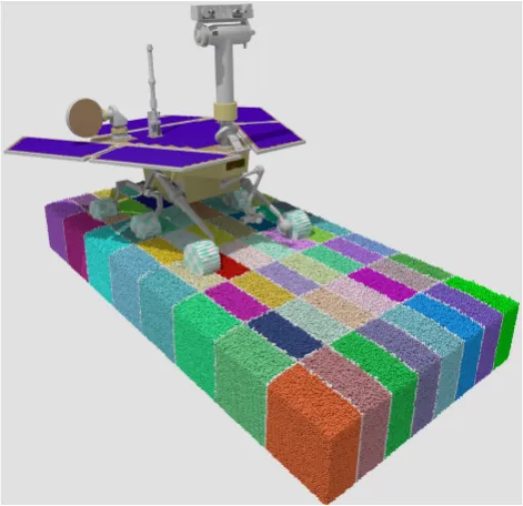
In this example we simulate a Mars Rover type wheeled vehicle operating on granular terrain. The vehicle is com-posed of a chassis and six wheels connected via revolute joints. The wheels are driven with a constant angular velocity of πrad s−1_{. The granular terrain is composed of 2 016 000}

spherical particles. The simulation is divided into 64 sub-domains and uses a time step of 10−5s. This small time step is necessary due to the use of the DEM approach to compute contact forces – a stiffforce model is used to achieve small normal interpenetration, requiring a small step size to main-tain stability. A snapshot from the simulation can be seen in Fig. 8. In the figure, note that the wheels of the rover are checkered blue and white. This signifies that the master copy of the rover assembly is in the blue sub-domain and the rover spans into adjacent sub-domains. In Fig. 8, the rover has set-tled into the granular terrain and is starting to move forward. The rear wheels displace more granular material than the front wheels because the center of mass of the rover is closer to the rear of the vehicle.

2.4 Validation and demonstration of technology

This section describes a validation effort in which experi-mental results were compared to simulation results obtained fromChrono::Engine. To this end, a test rig was designed and fabricated to measure the rate at which granular material flowed out of a slit due to gravity.Chrono::Engine was used to set up a corresponding simulation to match the experimen-tal results. For more detail, see Melanz et al. (2010).

2.4.1 Experimental model

The experimental set-up consisted of a fixed base, a mov-able wall (angled at 45◦_{), a translational stage, a linear}

tuator, and a scale (see schematic in Fig. 9). The linear ac-tuator was capable of quickly opening a precise gap, out of which the granular material would flow due to gravity. The

(8)

Mazhar et al.:

Chrono

7

Figure 8

: Snapshot of Mars Rover simulation with 2,016,000

ter-rain particles using 64 domains. Bodies are colored by

sub-domain, with shared bodies (those which span sub-domain

bound-aries) colored white.

and fabricated to measure the rate at which granular material

flowed out of a slit due to gravity.

Chrono

::Engine was used

to set up a corresponding simulation to match the

experimen-tal results. For more detail, see (Melanz et al., 2010).

2.4.1

Experimental Model

The experimental set-up consisted of a fixed base, a movable

wall (angled at 45

◦

), a translational stage, a linear actuator,

and a scale (see schematic in Fig. 9). The linear actuator

was capable of quickly opening a precise gap, out of which

the granular material would flow due to gravity. The scale

recorded the mass of collected granular material as a function

of time. The granular material consisted of approximately

40,000 uniform glass disruptor beads with diameter of 500

microns. Experiments were performed for gap sizes of 1.5

mm, 2 mm, 2.5 mm, and 3 mm. At least 5 experiments were

performed for each gap size.

2.4.2

Simulation Model

Chrono

::Engine was used to build a model representing the

experimental set up described above.

In the model, the

trough was represented by four rectangular boxes of finite

dimensions. The motion of the box representing the angled

side was captured from the data sheet of the translational

stage. The granular material was modeled as perfect,

identi-cal spheres with the same mass and coe

ffi

cient of friction.

The load cell measured the outflow through the gap. In the

simulation, the scale was modeled by counting the number

of spheres below a certain height. The number of spheres

Figure 9

: Schematic of validation experiment. A linear actuator

and translational stage moved the left angled side a fixed amount,

opening a precise gap from which the particles flowed. The mass

flow rate was measured by the scale. Schematic not to scale.

multiplied by the mass and gravity yielded the weight which

was compared with experimental results. A plane was used

to contain the spheres after they had been counted.

In order to save computational time, the simulation was split

into two parts: one representing the process of filling the

trough and the other the opening and measuring process.

In this way, the trough was filled with randomly positioned

spheres which were allowed to settle. Once the kinetic

en-ergy of the system was below 0.001 Joules and had reached

a relatively constant value, the x-, y- , and z-position of each

sphere was saved to a file.

The same initial conditions from the settling simulation were

used to perform all of the necessary simulations. At the

be-ginning of each simulation the position data set of the spheres

was loaded into the model and the spheres were created at the

same positions they appeared in the filling process. The

mo-tion was applied to the translating side to achieve the desired

gap size, and the material began to flow.

The simulations setup consisted of 39,000 rigid body spheres

with a radius of 2

.

5

×

10

−4

m and a mass of 1

.

631

×

10

−7

kg.

The following parameters were set for this simulation. A

time step of 10

−4

[s] with 500 CCP iterations, and a tolerance

of 10

−7

for the maximum velocity correction. Simulations

were generally run for 8 seconds. SI units were used for all

parameters.

2.4.3

Procedure Used to Select the Friction Coefficient

The friction coe

ffi

cient of a certain material is not a constant

value. It can depend on various environmental influences

such as humidity, surface quality, temperature etc. The

fric-www.mech-sci.net

Mech. Sci.

Figure 8.Snapshot of Mars Rover simulation with 2 016 000 terrain particles using 64 sub-domains. Bodies are colored by sub-domain, with shared bodies (those which span sub-domain boundaries) col-ored white.

Mazhar et al.:Chrono: A Parallel Multi-Physics Library for Rigid-Body, Flexible-Body, and Fluid Dynamics 7

Figure 8: Snapshot of Mars Rover simulation with 2,016,000 ter-rain particles using 64 domains. Bodies are colored by sub-domain, with shared bodies (those which span sub-domain bound-aries) colored white.

and fabricated to measure the rate at which granular material flowed out of a slit due to gravity.Chrono::Engine was used to set up a corresponding simulation to match the experimen-tal results. For more detail, see (Melanz et al., 2010).

2.4.1 Experimental Model

The experimental set-up consisted of a fixed base, a movable wall (angled at 45◦), a translational stage, a linear actuator, and a scale (see schematic in Fig. 9). The linear actuator was capable of quickly opening a precise gap, out of which the granular material would flow due to gravity. The scale recorded the mass of collected granular material as a function of time. The granular material consisted of approximately 40,000 uniform glass disruptor beads with diameter of 500 microns. Experiments were performed for gap sizes of 1.5 mm, 2 mm, 2.5 mm, and 3 mm. At least 5 experiments were performed for each gap size.

2.4.2 Simulation Model

Chrono::Engine was used to build a model representing the

experimental set up described above. In the model, the trough was represented by four rectangular boxes of finite dimensions. The motion of the box representing the angled side was captured from the data sheet of the translational stage. The granular material was modeled as perfect, identi-cal spheres with the same mass and coefficient of friction. The load cell measured the outflow through the gap. In the simulation, the scale was modeled by counting the number of spheres below a certain height. The number of spheres

Figure 9: Schematic of validation experiment. A linear actuator and translational stage moved the left angled side a fixed amount, opening a precise gap from which the particles flowed. The mass flow rate was measured by the scale. Schematic not to scale.

multiplied by the mass and gravity yielded the weight which was compared with experimental results. A plane was used to contain the spheres after they had been counted.

In order to save computational time, the simulation was split into two parts: one representing the process of filling the trough and the other the opening and measuring process. In this way, the trough was filled with randomly positioned spheres which were allowed to settle. Once the kinetic en-ergy of the system was below 0.001 Joules and had reached a relatively constant value, the x-, y- , and z-position of each sphere was saved to a file.

The same initial conditions from the settling simulation were used to perform all of the necessary simulations. At the be-ginning of each simulation the position data set of the spheres was loaded into the model and the spheres were created at the same positions they appeared in the filling process. The mo-tion was applied to the translating side to achieve the desired gap size, and the material began to flow.

The simulations setup consisted of 39,000 rigid body spheres with a radius of 2.5×10−4_{m and a mass of 1}_.₆₃₁_×₁₀−7_kg.

The following parameters were set for this simulation. A time step of 10−4_{[s] with 500 CCP iterations, and a tolerance}

of 10−7 for the maximum velocity correction. Simulations were generally run for 8 seconds. SI units were used for all parameters.

2.4.3 Procedure Used to Select the Friction Coefficient

The friction coefficient of a certain material is not a constant value. It can depend on various environmental influences such as humidity, surface quality, temperature etc. The

fric-www.mech-sci.net Mech. Sci.

Figure 9.Schematic of validation experiment. A linear actuator and translational stage moved the left angled side a fixed amount, open-ing a precise gap from which the particles flowed. The mass flow rate was measured by the scale. Schematic not to scale.

scale recorded the mass of collected granular material as a function of time. The granular material consisted of approx-imately 40 000 uniform glass disruptor beads with diameter of 500 microns. Experiments were performed for gap sizes of 1.5 mm, 2 mm, 2.5 mm, and 3 mm. At least 5 experiments were performed for each gap size.

2.4.2 Simulation model

Chrono::Engine was used to build a model representing the experimental set up described above. In the model, the trough was represented by four rectangular boxes of finite dimen-sions. The motion of the box representing the angled side was captured from the data sheet of the translational stage. The granular material was modeled as perfect, identical spheres with the same mass and coefficient of friction.

The load cell measured the outflow through the gap. In the simulation, the scale was modeled by counting the number of spheres below a certain height. The number of spheres multiplied by the mass and gravity yielded the weight which was compared with experimental results. A plane was used to contain the spheres after they had been counted.

In order to save computational time, the simulation was split into two parts: one representing the process of filling the trough and the other the opening and measuring process. In this way, the trough was filled with randomly positioned spheres which were allowed to settle. Once the kinetic en-ergy of the system was below 0.001 Joules and had reached a relatively constant value, the x-, y- , and z-position of each sphere was saved to a file.

The same initial conditions from the settling simulation were used to perform all of the necessary simulations. At the beginning of each simulation the position data set of the spheres was loaded into the model and the spheres were cre-ated at the same positions they appeared in the filling process. The motion was applied to the translating side to achieve the desired gap size, and the material began to flow.

The simulations setup consisted of 39 000 rigid body spheres with a radius of 2.5×10−4m and a mass of 1.631×

10−7_{kg. The following parameters were set for this}

simula-tion. A time step of 10−4_{s with 500 CCP iterations, and a}

tolerance of 10−7_{for the maximum velocity correction.}

Sim-ulations were generally run for 8 s. SI units were used for all parameters.

2.4.3 Procedure used to select the friction coefficient

The friction coefficient of a certain material is not a con-stant value. It can depend on various environmental influ-ences such as humidity, surface quality, temperature etc. The friction coefficient of glass was an unknown in the validation process and needed to be determined before further obser-vations could be done. To achieve this, one experiment at a gap size of 1.5 mm was performed and multiple simulations with the same setup and different friction coefficients were performed. The simulation results were compared to the ex-perimental test results to determine which friction coefficient resulted in the best match, see Fig. 10. It was determined that

µ=0.15 most closely matched the experimental results. This value was used for all subsequent simulations.

(9)

8

Mazhar et al.:

Chrono

Figure 10

: Selection of

µ

Figure 11

: Weight vs time for a gap size of 3 mm.

tion coe

ffi

cient of glass was an unknown in the validation

process and needed to be determined before further

obser-vations could be done. To achieve this, one experiment at a

gap size of 1.5 mm was performed and multiple simulations

with the same setup and di

ff

erent friction coe

ffi

cients were

performed. The simulation results were compared to the

ex-perimental test results to determine which friction coe

ffi

cient

resulted in the best match, see Fig. 10. It was determined that

µ

=

0

.

15 most closely matched the experimental results. This

value was used for all subsequent simulations.

2.4.4

Results

The weight of the collected granular material is plotted

ver-sus time for various gap sizes in Fig. 11 through Fig. 14 using

the friction coe

ffi

cient determined in Fig. 10. For each

ex-periment, the result from the simulation in

Chrono

::Engine,

shown by the solid line, is overlaid on top of the standard

de-viation of the experimental runs, shown by the dashed line.

Note that the simulated result lies within a single standard

deviation of the experimental data.

Figure 12

: Weight vs time for a gap size of 2.5 mm.

Figure 13

3

Chrono::Flex

The

Chrono

::Flex software is a general-purpose simulator

for three dimensional flexible multi-body problems and

pro-vides a suite of flexible body support. The features included

in this module are multiple element types, the ability to

con-nect these elements with a variety of bilateral constraints,

multiple solvers, and contact with friction.

Additionally,

Chrono

::Flex leverages the GPU to accelerate solution of

large problems.

3.1

Element Types

Chrono

::Flex includes two element types implemented

us-ing the Absolute Nodal Coordinate Formulation (ANCF)

Berzeri et al. (2001); von Dombrowski (2002). The

gradient-deficient beam element and the gradient-gradient-deficient plate

ele-ment are described below.

3.1.1

Gradient-Deficient Beam Elements

This implementation uses gradient deficient ANCF beam

ele-ments to model slender beams, examples of which are shown

in Figure 15. These are two node elements with one position

vector and only one gradient vector used as nodal

coordi-nates. Each node thus has 6 coordinates: three components

Mech. Sci.

www.mech-sci.net

Figure 10.Selection ofµ.

8

Mazhar et al.:

Chrono

Figure 10

: Selection of

µ

Figure 11

tion coe

ffi

obser-vations could be done. To achieve this, one experiment at a

with the same setup and di

ff

erent friction coe

ffi

cients were

ffi

cient

µ

=

0

.

value was used for all subsequent simulations.

2.4.4

Results

the friction coe

ffi

Chrono

::Engine,

deviation of the experimental data.

Figure 12

Figure 13

: Weight vs time for a gap size of 2 mm.

3

Chrono::Flex

The

Chrono

in this module are multiple element types, the ability to

con-nect these elements with a variety of bilateral constraints,

Additionally,

Chrono

large problems.

3.1

Element Types

Chrono

us-ing the Absolute Nodal Coordinate Formulation (ANCF)

Berzeri et al. (2001); von Dombrowski (2002). The

3.1.1

in Figure 15. These are two node elements with one position

Mech. Sci.

www.mech-sci.net

Figure 11.Weight vs. time for a gap size of 3 mm.

2.4.4 Results

The weight of the collected granular material is plotted ver-sus time for various gap sizes in Fig. 11 through Fig. 14 using the friction coefficient determined in Fig. 10. For each ex-periment, the result from the simulation inChrono::Engine, shown by the solid line, is overlaid on top of the standard de-viation of the experimental runs, shown by the dashed line. Note that the simulated result lies within a single standard deviation of the experimental data.

3 Chrono::Flex

The Chrono::Flex software is a general-purpose simula-tor for three dimensional flexible multi-body problems and provides a suite of flexible body support. The features in-cluded in this module are multiple element types, the abil-ity to connect these elements with a variety of bilateral con-straints, multiple solvers, and contact with friction.

Addition-8

Mazhar et al.:

Chrono

Figure 10

: Selection of

µ

Figure 11

tion coe

ffi

obser-vations could be done. To achieve this, one experiment at a

with the same setup and di

ff

erent friction coe

ffi

cients were

ffi

cient

µ

=

0

.

value was used for all subsequent simulations.

2.4.4

Results

the friction coe

ffi

Chrono

::Engine,

deviation of the experimental data.

Figure 12

Figure 13

3

Chrono::Flex

The

Chrono

in this module are multiple element types, the ability to

con-nect these elements with a variety of bilateral constraints,

Additionally,

Chrono

large problems.

3.1

Element Types

Chrono

us-ing the Absolute Nodal Coordinate Formulation (ANCF)

Berzeri et al. (2001); von Dombrowski (2002). The

3.1.1

in Figure 15. These are two node elements with one position

Mech. Sci.

www.mech-sci.net

Figure 12.Weight vs. time for a gap size of 2.5 mm.

8

Mazhar et al.:

Chrono

Figure 10

: Selection of

µ

Figure 11

tion coe

ffi

obser-vations could be done. To achieve this, one experiment at a

with the same setup and di

ff

erent friction coe

ffi

cients were

ffi

cient

µ

=

0

.

value was used for all subsequent simulations.

2.4.4

Results

the friction coe

ffi

Chrono

::Engine,

deviation of the experimental data.

Figure 12

Figure 13

: Weight vs time for a gap size of 2 mm.

3

Chrono::Flex

The

Chrono

in this module are multiple element types, the ability to

con-nect these elements with a variety of bilateral constraints,

Additionally,

Chrono

large problems.

3.1

Element Types

Chrono

us-ing the Absolute Nodal Coordinate Formulation (ANCF)

Berzeri et al. (2001); von Dombrowski (2002). The

3.1.1

in Figure 15. These are two node elements with one position

Mech. Sci.

www.mech-sci.net

Figure 13.Weight vs. time for a gap size of 2 mm.

ally,Chrono::Flex leverages the GPU to accelerate solution of large problems.

3.1 Element types

Chrono::Flex includes two element types implemented us-ing the Absolute Nodal Coordinate Formulation (ANCF) (Berzeri et al., 2001; von Dombrowski, 2002). The gradient-deficient beam element and the gradient-gradient-deficient plate ele-ment are described below.

3.1.1 Gradient-deficient beam elements

This implementation uses gradient deficient ANCF beam ele-ments to model slender beams, examples of which are shown in Fig. 15. These are two node elements with one position vector and only one gradient vector used as nodal coordi-nates. Each node thus has 6 coordinates: three components of the global position vector of the node and three compo-nents of the position vector gradient at the node. This formu-lation displays no shear locking problems for thin and stiff beams and is computationally more efficient compared to the original ANCF due to the reduced number of nodal coordi-nates (Gerstmayr and Shabana, 2006). The gradient deficient

(10)

Figure 14.Weight vs. time for a gap size of 1.5 mm. This was the test case that was used for calibration.

Figure 15. Two models with friction and contact using Chrono::Flex beam elements: a ball sitting on grass-like beams and a ball hitting a net.

ANCF beam element does not describe a rotation of the beam about its own axis so the torsional effects cannot be modeled.

3.1.2 Gradient-deficient plate elements

Much like beams, numerical difficulties are encountered in the fully parameterized plate element when the system has very thin and stiffcomponents (Dufva and Shabana, 2005). The high frequencies that are induced along the thin direction of the element require an extremely small time step, resulting in longer simulation times. In the case where the aspect ratio (length divided by thickness) of the element is high, plane stress assumptions can be made that allow a reduced-order element to be accurate. Specifically, Kirchhoff’s plate theory, which does not account for shear deformation, is used and results in an element with 36 degrees of freedom, or nodal coordinates, are shown in Fig. 16.

3.2 Kinematic constraints

Several types of mechanical joints are modeled in

Chrono::Flex. A spherical joint (Shabana, 2005) between two nodes of an