Block-Based Adaptive Vector Lifting Schemes for Multichannel Image Coding

Volume 2007, Article ID 13421,10pages doi:10.1155/2007/13421

Research Article

Block-Based Adaptive Vector Lifting Schemes for

Multichannel Image Coding

Amel Benazza-Benyahia,1_{Jean-Christophe Pesquet,}2_{Jamel Hattay,}1_{and Hela Masmoudi}3, 4

1_{Unit´e de Recherche en Imagerie Satellitaire et ses Applications (URISA), Ecole Sup´erieure des Communications}

(SUP’COM), Tunis 2083, Tunisia

2_{Institut Gaspard Monge and CNRS-UMR 8049, Universit´e de Marne la Vall´ee, 77454 Marne la Vall´ee C´edex 2, France} 3_{Department of Electrical and Computer Engineering, George Washington University, Washington, DC 20052, USA}

4_{US Food and Drug Administration, Center of Devices and Radiological Health, Division of Imaging and Applied Mathematics,}

Rockville, MD 20852, USA

Received 28 August 2006; Revised 29 December 2006; Accepted 2 January 2007

Recommended by E. Fowler

We are interested in lossless and progressive coding of multispectral images. To this respect, nonseparable vector lifting schemes are used in order to exploit simultaneously the spatial and the interchannel similarities. The involved operators are adapted to the image contents thanks to block-based procedures grounded on an entropy optimization criterion. A vector encoding technique derived from EZW allows us to further improve the efficiency of the proposed approach. Simulation tests performed on remote sensing images show that a significant gain in terms of bit rate is achieved by the resulting adaptive coding method with respect to the non-adaptive one.

Copyright © 2007 Amel Benazza-Benyahia et al. This is an open access article distributed under the Creative Commons Attribution License, which permits unrestricted use, distribution, and reproduction in any medium, provided the original work is properly cited.

1. INTRODUCTION

The interest in multispectral imaging has been increasing in many fields such as agriculture and environmental sciences. In this context, each earth portion is observed by several

sen-sors operating at different wavelengths. By gathering all the

spectral responses of the scene, a multicomponent image is obtained. The spectral information is valuable for many ap-plications. For instance, it allows pixel identification of ma-terials in geology and the classification of vegetation type in agriculture. In addition, the long-term storage of such images is highly desirable in many applications. However, it con-stitutes a real bottleneck in managing multispectral image databases. For instance, in the Landsat 7 Enhanced Thematic Mapper Plus system, the 8-band multispectral scanning ra-diometer generates 3.8 Gbits per scene with a data rate of 150 Mbps. Similarly, the Earth Orbiter I (EO-I) instrument works at a data bit rate of 500 Mbps. The amount of data will continue to become larger with the increase of the num-ber of spectral bands, the enhancement of the spatial reso-lution, and the improvement of the radiometry accuracy re-quiring finer quantization steps. It is expected that the next

Landsat generation will work at a data rate of several Gbps. Hence, compression becomes mandatory when dealing with multichannel images. Several methods for data reduction are available, the choice strongly depend on the underlying

ap-plication requirements [1]. Generally, on-board compression

techniques are lossy because the acquisition data rates exceed the downlink capacities. However, ground coding methods are often lossless so as to avoid distortions that could dam-age the estimated values of the physical parameters corre-sponding to the sensed area. Besides, scalability during the browsing procedure constitutes a crucial feature for ground information systems. Indeed, a coarse version of the image is firstly sent to the user to make a decision about whether to abort the decoding if the data are considered of little in-terest or to continue the decoding process and refine the visual quality by sending additional information. The chal-lenge for such progressive decoding procedure is to design a compact multiresolution representation. Lifting schemes

(LS) have proved to be efficient tools for this purpose [2,3].

Generally, the 2D LS is handled in a separable way. Recent works have however introduced nonseparable quincunx

generation of coders following nonrectangularly subsampled

filterbanks [5–7]. These schemes are motivated by the

emer-gence of quincunx sampling image acquisition and display

devices such as in the SPOT5 satellite system [8]. Besides,

nonseparable decompositions offer the advantage of a “true”

two-dimensional processing of the images presenting more degrees of freedom than the separable ones. A key issue of such multiresolution decompositions (both LS and QLS) is the design of the involved decomposition operators. Indeed, the performance can be improved when the intrinsic spatial properties of the input image are accounted for. A possible adaptation approach consists in designing space-varying fil-ter banks based on conventional adaptive linear mean square

algorithms [9–11]. Another solution is to adaptively choose

the operators thanks to a nonlinear decision rule using the

local gradient information [12–15]. In a similar way,

Taub-man proposed to adapt the vertical operators for reducing the edge artifacts especially encountered in compound

doc-uments [16]. Boulgouris et al. have computed the optimal

predictors of an LS in the case of specific wide-sense station-ary fields by considering an a priori autocovariance model of

the input image [17]. More recently, adaptive QLS have been

built without requiring any prior statistical model [8] and, in

[18], a 2D orientation estimator has been used to generate an

edge adaptive predictor for the LS. However, all the reported works about adaptive LS or QLS have only considered mono-component images. In the case of multimono-component images, it is often implicitly suggested to decompose separately each component. Obviously, an approach that takes into account the spectral similarities in addition to the spatial ones should

be more efficient than the componentwise approach. A

pos-sible solution as proposed in Part 2 of the JPEG2000

stan-dard [19] is to apply a reversible transform operating on the

multiple components before their spatial multiresolution de-composition. In our previous work, we have introduced the

concept ofvectorlifting schemes (VLS) that decompose

si-multaneouslyall the spectral components in a separable

man-ner [20] or in a nonseparable way (QVLS) [21]. In this paper,

we consider blockwise adaptation procedures departing from the aforementioned adaptive approaches. Indeed, most of the existing works propose a pointwise adaptation of the opera-tors, which may be costly in terms of bit rate.

More precisely, we propose to firstly segment the image into nonoverlapping blocks which are further classified into

several regions corresponding to different statistical features.

The QVLS operators are then optimally computed for each region. The originality of our approach relies on the opti-mization of a criterion that operates directly on the entropy, which can be viewed as a sparsity measure for the multireso-lution representation.

This paper is organized as follows. InSection 2, we

pro-vide preliminaries about QVLS. The issue of the adaptation

of the QVLS operators is addressed inSection 3. The

objec-tive of this section is to design efficient adaptive

multireso-lution decompositions by modifying the basic structure of the QVLS. The choice of an appropriate encoding technique

is also discussed in this part. InSection 4, experimental

re-sults are presented showing the good performance of the

x o x o x o x o o x o x o x o x x o x o x o x o o x o x o x o x x o x o x o x o o x o x o x o x

Figure 1: Quincunx sampling grid: the polyphase components

x(0b)(m,n) correspond to the “x” pixels whereas the polyphase com-ponentsx(0b)(m,n) correspond to the “o” pixels.

proposed approach. A comparison of the fixed and variable block size strategies is also performed. Finally, some

conclud-ing remarks are given inSection 5.

2. VECTOR QUINCUNX LIFTING SCHEMES

2.1. The lifting principle

In a generic LS, the input image is firstly split into two sets

S1andS2of spatial samples. Because of the local correlation,

a predictor (P) allows to predict theS1samples from theS2

ones and to replace them by their prediction errors. Finally,

theS2samples are smoothed using the residual coefficients

thanks to an update (U) operator. The updated coefficients

correspond to a coarse version of the input signal and, a mul-tiresolution representation is then obtained by recursively re-peating this decomposition to the updated approximation

coefficients. The main advantage of the LS is its reversibility

regardless of the choice of the P and U operators. Indeed, the inverse transform is simply obtained by reversing the order of the operators (U-P) and substituting a minus (resp., plus) sign by a plus (resp., minus) one. Thus, the LS can be con-sidered as an appealing tool for exact and progressive coding. Generally, the LS is applied to images in a separable manner as for instance in the 5/3 wavelet transform retained for the JPEG2000 standard.

2.2. Quincunx lifting scheme

More general LS can be obtained with nonseparable

decom-positions giving rise to the so-called QLS [4]. In this case,

theS1andS2sets, respectively, correspond to the two

quin-cunx polyphase componentsx(j/b2)(m,n) andx(j/b2)(m,n) of the

approximationa(j/b2)(m,n) of thebth band at resolution j/2

(with j∈N):

x(j/b2)(m,n)=a(j/b2)(m−n,m+n),

x(j/b2)(m,n)=a(j/b2)(m−n+ 1,m+n),

(1)

where (m,n) denotes the current pixel. The initialization

is performed at resolution j = 0 by taking the polyphase

components of the original image x(n,m) when this one

has been rectangularly sampled (seeFigure 1). We have then

a0(n,m) = x(n,m). If the quincunx subsampled version of

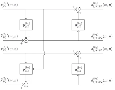
x(b1)

j/2(m,n) ₊ +

+ a(b1)

(j+1)/2(m,n)

p(b1)

j/2 u(j/b21)

x(b1)

j/2(m,n) − + +

d(b1) (j+1)/2(m,n) x(b2)

j/2(m,n) ₊ +

+ a(b2)

(j+1)/2(m,n)

p(b2)

j/2 u(j/b22)

x(b2)

j/2(m,n) − + +

d(b2) (j+1)/2(m,n)

Figure2: An example of a decomposition vector lifting scheme in

the case of a two-channel image.

resolutionj=1/2 by settinga(1b/)2(n,m)=x(b)(m−n,m+n).

In the P step, the prediction errorsd((bj+1)) /2(m,n) are

com-puted:

d((bj+1)) /2(m,n)=x (b)

j/2(m,n)−

x(_j/b₂)(m,n)p(_j/b₂), (2)

where · is a rounding operator, x(_j/b2)(m,n) is a vector

containing some a(j/b2)(m,n) samples, and, p (b)

j/2 is a vector

of prediction weights of the same size. The approximation

a((bj+1)) /2(m,n) ofa (b)

j/2(m,n) is an updated version ofx (b)

j/2(m,n)

using some of thed((bj+1)) /2(m,n) samples regrouped into the

vectord(_j/b2)(m,n):

a((bj+1)) /2(m,n)=x (b)

j/2(m,n) +

d(_j/b2)(m,n)u(j/b)2

, (3)

whereu(_j/b2)is the associated update weight vector. The

result-ing approximation can be further decomposed so as to get a multiresolution representation of the initial image. Unlike classical separable multiresolution analyses where the input signal is decimated by a factor 4 to generate the approxima-tion signal, the number of pixels is divided by 2 at each (half-) resolution level of the nonseparable quincunx analysis.

2.3. Vector quincunx lifting scheme

The QLS can be extended to a QVLS in order to exploit the interchannel redundancies in addition to the spatial ones. More precisely, thed(j/b2)(m,n) anda

(b)

j/2(m,n) coefficients are

now obtained by using coefficients of the considered band

bandalso coefficients of theotherchannels. Obviously, the

QVLS represents a versatile framework, the QLS being a special case. Besides, the QVLS is quite flexible in terms of selection of the prediction mask and component ordering.

Figure 2shows the corresponding analysis structures. As an example of particular interest, we will consider the simple QVLS whose P operator relies on the following neighbors of

the coefficienta(j/b2)(m−n+ 1,m+n):

x(b1)

j/2(m,n)=

⎛ ⎜ ⎜ ⎜ ⎜ ⎜ ⎜ ⎝

a(b1)

j/2(m−n,m+n) a(b1)

j/2(m−n+ 1,m+n−1) a(b1)

j/2(m−n+ 1,m+n+ 1) a(b1)

j/2(m−n+ 2,m+n)

⎞ ⎟ ⎟ ⎟ ⎟ ⎟ ⎟ ⎠ ,

∀i >1, x(bi)

j/2(m,n)=

⎛ ⎜ ⎜ ⎜ ⎜ ⎜ ⎜ ⎜ ⎜ ⎜ ⎜ ⎜ ⎜ ⎜ ⎜ ⎜ ⎜ ⎜ ⎜ ⎜ ⎝

a(bi)

j/2(m−n,m+n) a(bi)

j/2(m−n+ 1,m+n−1) a(bi)

j/2(m−n+ 1,m+n+ 1) a(bi)

j/2(m−n+ 2,m+n)

a(bi−1)

j/2 (m−n+ 1,m+n)

.. .

a(b1)

j/2(m−n+ 1,m+n)

⎞ ⎟ ⎟ ⎟ ⎟ ⎟ ⎟ ⎟ ⎟ ⎟ ⎟ ⎟ ⎟ ⎟ ⎟ ⎟ ⎟ ⎟ ⎟ ⎟ ⎠ , (4)

where (b1,. . .,bB) is a given permutation of the channel

in-dices (1,. . .,B). Thus, the componentb1, which is chosen as a

reference channel, is coded by making use of a purely spatial

predictor. Then, the remaining componentsbi(fori >1) are

predicted both from neighboring samples of the same

com-ponentbi(spatial mode)andfrom the samples of the

previ-ous componentsbk(fork < i) located at the same position.

The final step corresponds to the following update, which is similarly performed for all the channels:

d(bi)

j/2(m,n)=

⎛ ⎜ ⎜ ⎜ ⎜ ⎜ ⎜ ⎝

d(bi)

j/2(m−1,n+ 1) d(bi)

j/2(m,n) d(bi)

j/2(m−1,n) d(bi)

j/2(m,n+ 1)

⎞ ⎟ ⎟ ⎟ ⎟ ⎟ ⎟ ⎠ . (5)

Note that such a decomposition structure requires to set

4B+ (B−1)B/2 parameters for the prediction weights and

4Bparameters for the update weights. It is worth

mention-ing that the update filter feeds the cross-channel information

back to the approximation coefficients since the detail

coef-ficients contain information from other channels. This may appear as an undesirable situation that may lead to some

leakage effects. However, due to the strong correlation

be-tween the channels, the detail coefficients of theBchannels

have a similar frequency content and no quality degradation was observed in practice.

3. ADAPTATION PROCEDURES

3.1. Entropy criterion

The compression ability of a QVLS-based representation de-pends on the appropriate choice of the P and U operators. In

general, the mean entropyHJ is a suitable measure of

com-pactness of theJ-stage multiresolution representation. This

algorithm is defined as the average of the entropiesH_J(b)of

theBchannel data:

HJ 1

B

B

b=1

H(b)

J . (6)

Likewise,H_J(b)is calculated as a weighted average of the

en-tropies of the approximation and the detail subbands:

H(b)

J

_J

j=1

2−j_H(b)

d,j/2

+ 2−J_H(b)

a,J/2, (7)

whereH_d(b_,j/)₂(resp.,H_a(_,b_J/)₂) denotes the entropy of the detail

(resp., approximation) coefficients of thebth channel, at

res-olution level j/2.

3.2. Optimization criteria

As mentioned inSection 1, the main contribution of this

pa-per is the introduction of some adaptivity rules in the QVLS

schemes. More precisely, the parameter vectorsp(_j/b₂)are

mod-ified according to the local activity of each subband. For this purpose, we have envisaged block-based approaches which start by partitioning each subband of each spectral

compo-nent into blocks. Then, for a given channel b, appropriate

classification procedures are applied in order to cluster the blocks which can use the same P and U operators within a given classc∈ {1,. . .,C(j/b2)}. It is worth pointing out that the

partition is very flexible as it depends on the considered spec-tral channel. In other words, the block segmentation yields

different maps from a channel to another. In this context, the

entropyH_d(b_,j/)₂is expressed as follows:

H(b)

d,j/2=

C(j/b2)

c=1 π(j/b2,c)H

(b,c)

d,j/2, (8)

whereH_d(b_,j/,c₂)denotes the entropy of the detail coefficients of

thebth channel within classcand, the weighting factorπ(j/b2,c)

corresponds to the probability that a detail sampled(j/b2)falls

into classc. Two problems are subsequently addressed: (i) the

optimization of the QVLS operators, (ii) the choice of the block segmentation method.

3.3. Optimization of the predictors

We now explain how a specific statistical modeling of the

detail coefficients within a classc can be exploited to effi

-ciently optimize the prediction weights. Indeed, the detail co-efficientsd((bj+1)) /2are often viewed as realizations of a

contin-uous zero mean random variableXwhose probability

den-sity functionfis given by a generalized Gaussian distribution

(GGD) [22,23]:

∀x∈R, fx;α((bj+1),c)/2,β (b,c) (j+1)/2

= β

(b,c) (j+1)/2

2α((bj,+1)c)/2Γ

1/β((bj,+1)c)/2

e−(|x|/α((jb,+1)c)/2)

β((bj,+1)c)/2

,

(9)

whereΓ(z)₀+∞tz−1_e−t_dt,α(b,c)

(j+1)/2>0 is the scale

parame-ter, andβ((bj+1),c)/2>0 is the shape parameter. These parameters

can be easily estimated from the empirical moments of the

data samples [24]. The GGD model allows to express the

dif-ferential entropyH(α((bj,+1)c)/2,β (b,c)

(j+1)/2) as follows:

Hα((bj,+1)c)/2,β (b,c) (j+1)/2

=log

₂

α((bj,+1)c)/2Γ

1/β((bj+1),c)/2

β((bj+1),c)/2

+ 1

β((bj+1),c)/2 .

(10)

It is worth noting that the proposed lifting structure

gener-ates integer-valued coefficients that can be viewed as

quan-tized versions of the continuous random variableX with a

quantization step q = 1. According to high rate

quantiza-tion theory [25], the differential entropyH(α((bj+1),c)/2,β (b,c) (j+1)/2)

provides a good estimate ofH_d(b_,j/,c)₂. In practice, the following

empirical estimator of the detail coefficients entropy is

em-ployed:

H_d,K(b,c)

j/2

α((bj+1),c)/2,β (b,c) (j+1)/2

= − 1

K(j/b2,c)

K(j/b2,c)

k=1

logfx(j/b2,c)(k)−

x(_j/b2,c)(k)

p(_j/b,2c)

,

(11)

wherex(j/b2,c)(1),. . .,x(j/b2,c)(Kj/(b2,c)) andx(j/b2,c)(1),. . .,x(j/b,2c)(K(j/b2,c))

areKj/(b2,c) ∈ N∗ realizations ofx (b)

j/2 andx (b)

j/2 classified inc.

As we aim at designing the most compact representation,

the objective is to compute the predictor p(_j/b2,c) that

mini-mizesHJ. From (6), (7), and (8), it can be deduced that the

optimal parameter vector also minimizesH_d(b_,j/)₂ and

there-fore,H(α((bj,+1)c)/2,β (b,c)

(j+1)/2), which is consistently estimated by

H_d,K(b,c) (j+1)/2(α

(b,c) (j+1)/2,β

(b,c)

(j+1)/2). This leads to the maximization of

Lp(_j/b,2c);α((bj+1),c)/2,β (b,c) (j+1)/2

= K(j/b2,c)

k=1

logfx(j/b2,c)(k)−

x(_j/b2,c)(k)

p(_j/b2,c)

.

(12)

Thus, the maximum likelihood estimator of p(_j/b₂,c) must be

determined. From (9), we deduce that the optimal predictor

minimizes the followingβ((bj+1),c)/2_criterion:

β((bj,+1)c)/2

p(_j/b2,c);α (b,c) (j+1)/2,β

(b,c) (j+1)/2

K(j/b2,c)

k=1

x(j/b2,c)(k)−

xj/2(k)(b,c)

p(_j/b2,c)

β((bj+1),c)/2

.

Hence, thanks to the GGD model, it is possible to design a

predictor in each classcthat ensures the compactness of the

representation in terms of the resulting detail subband en-tropy. However, it has been observed that the considered sta-tistical model is not always adequate for the approximation subbands which makes impossible to derive a closed form ex-pression for the approximation subband entropy. Related to this fact, several alternatives can be envisaged for the selec-tion of the update operator. For instance, it can be adapted to the contents of the image so as to minimize the

reconstruc-tion error [8]. It is worth noticing that, in this case, the

un-derlying criterion is the variance of the reconstruction error and not the entropy. A simpler alternative that we have re-tained in our experiments consists in choosing the same up-date operator for all the channels, resolution levels, and clus-ters. Indeed, in our experiments, it has been observed that the decrease of the entropy is mainly due to the optimization of the predictor operators.

3.4. Fixed-size block segmentation

The second ingredient of our adaptive approach is the block segmentation procedure. We have envisaged two alternatives.

The first one consists in iteratively classifyingfixedsize blocks

as follows [8].

INIT

The block size s(j/b)2×t(j/b2) and the number of regions C(j/b2)

are fixed by the user. Then, the approximation a(j/b)2 is

par-titioned into nonoverlapping blocks that are classified into

C(j/b2)regions. It should be pointed out that the classification

of the approximation subband has been preferred to that of

the detail subbands at a given resolution level j. Indeed, it is

expected that homogenous regions (in the spatial domain) share a common predictor, and such homogeneous regions are more easily detected from the approximation subbands than from the detail ones. For instance, a possible classifica-tion map can be obtained by clustering the blocks according to their mean values.

PREDICT

In each classc, the GGD parametersα((bj+1),c)/2and,β (b,c) (j+1)/2are

estimated as described in [24]. Then, the optimal predictor

p(_j/b,₂c)that minimizes theβ((bj,+1)c)/2_{criterion is derived. The}

ini-tial values of the predictor weights are set by minimizing the

detail coefficient variance.

ASSIGN

The contents of each classcare modified so that a block of

details initially in classccould be moved to another classc∗

according to some assignment criterion. More precisely, the global entropyH_d(b_,j/,c₂)is equal to the sum of the contributions

of all the detail blocks within classc. This additive property

enables to easily derive the optimal assignement rule. At each

resolution level and, according to the retained band ordering,

a current blockBis assigned to a classc∗if its contribution

to the entropy of that class induces the maximum decrease of

the global entropy. This amounts to move the blockB,

ini-tially assumed to belong to classc, to classc∗if the following

condition is satisfied:

hB,α((bj+1),c)/2,β (b,c) (j+1)/2

< hB,α((bj,+1)c∗)/2,β (b,c∗₎ (j+1)/2

, (14)

where

hB,α((bj,+1)c)/2,β (b,c) (j+1)/2

s(j/b)2

m=1

t(j/b)2

n=1

logfB(m,n);α((bj+1),c)/2,β (b,c) (j+1)/2

.

(15)

PREDICTandASSIGNsteps are repeated until the conver-gence of the global entropy. Then, the procedure is iterated

through theJresolution stages.

At the convergence of the procedure, at each resolution level, the chosen predictor for each block is identified with a binary index code which is sent to the decoder leading to an overall overhead not exceeding

o=

_B

b=1

J

j=1

log₂C(j/b2)

s(j/b2t)

(b)

j/2

(bpp). (16)

Note that the amount of side information can be further

re-duced by differential encoding.

3.5. Variable-size block segmentation

More flexibility can be achieved by varying the block sizes according to the local activity of the image. To this respect, a quadtree (QT) segmentation in the spatial domain is used which provides a layered representation of the regions in the image. For simplicity, this approach has been imple-mented using a volumetric segmentation (same segmenta-tion for each image channel at a given resolusegmenta-tion as depicted in Figure 3) [26]. The regions are obtained according to a

segmentation criterion R that is suitable for compression

purposes. Generally, the QT can be built following two al-ternatives: a splitting or a merging approach. The first one starts from a partition of the transformed multicomponent

image into volumetric quadrants. Then, each quadrant f is

split into 4 volumetric subblocksc1,. . .,c4if the criterionR

holds, otherwise the untouched quadrantf is associated with

a leaf of the unbalanced QT. The subdivision is eventually

repeated on the subblocksc1,. . .,c4until the subblock

min-imum sizek1×k2 is achieved. Finally, the resulting

block-shaped regions correspond to the leaves of the unbalanced QT.

In contrast, the initial step of the dual approach (i.e., the merging procedure) corresponds to a partition of the image

into minimum sizek1×k2subblocks. Then, the

homogene-ity with respect to the ruleR of each quadrant formed by

adjacent volumetric subblocks c1,. . .,c4 is checked. In case

of homogeneity, the fusion of c1,. . .,c4 is carried out,

B

sp

ect

ral

co

mponents

Figure3: An example of a volumetric block-partitioning of aB

-component image.

the fusion procedure is recursively performed until the whole image size is reached.

Obviously, the key issue of such QT partitioning lies in

the definition of the segmentation ruleR. In our work, this

rule is based on the lifting optimization criterion. Indeed, in the case of the splitting alternative, the objective is to decide

whether the splitting of a node f into its 4 childrenc1,. . .,c4

provides a more compact representation than the node f

does. For each channel, the optimal prediction and update weights p(_j/b,2f) u

(b,f)

j/2 of node f are computed for a J-stage

decomposition. The optimal weightsp(b,ci)

j/2 and,u (b,ci)

j/2 of the

childrenc1,. . .,c4are also computed. LetH_d(b_,j/,f₂)and,H(b,ci)

d,j/2

denote the entropy of the resulting multiresolution

represen-tations. The splitting is decided if the following inequalityR

holds:

1

4B

4

i=1

_B

b=1

H(b,ci)

d,j/2

+oci

< 1 B

_B

b=1

H(b,f)

d,j/2

+o(f),

(17)

where o(n) is the coding cost of the side information

re-quired by the decoding procedure at noden. This overhead

information concerns the tree structure and the operators weights. Generally, it is easy to code the QT by assigning the bit “1” to an intermediate node and the bit “0” to a leaf. Since the image corresponds to all the leaves of the QT, the prob-lem amounts to the coding of the binary sequences point-ing on these terminatpoint-ing nodes. To this respect, a run-length coder is used. Concerning the operators weights, these ones should be exactly coded. As they take floating values, they are rounded prior to the arithmetic coding stage. Obviously, to avoid any mismatch, the approximation and detail coef-ficients are computed according to these rounded weights. Finally, it is worth noting that the merging rule is derived in

a straightforward way from (17).

Table1: Description of the test images.

Name Number of_components Source Scene

Trento6 6 Thematic Mapper Rural Trento7 7 Thematic Mapper Rural

Tunis3 3 SPOT3 Urban

Kair4 4 SPOT4 Rural

Tunis4-160 4 SPOT4 Rural

Tunis4-166 4 SPOT4 Rural

Table2: Influence of the prediction optimization criterion on the

average entropies for non adaptive 4-level QLS and QVLS decom-positions. The update was fixed for all resolution levels and for all the components.

Image QLS

2

QLS

β Gain

QVLS

2

QVLS

β Gain

Trento6 4.2084 4.1172 0.0912 3.8774 3.7991 0.0783 Trento7 3.9811 3.8944 0.0867 3.3641 3.2988 0.0653 Tunis3 5.3281 5.2513 0.0768 4.5685 4.4771 0.0914 Kair4 4.3077 4.1966 0.1111 3.9222 3.8005 0.1217 Tunis4-160 4.7949 4.7143 0.0806 4.2448 4.1944 0.0504 Tunis4-166 3.9726 3.9075 0.0651 3.7408 3.6205 0.1203 Average 4.4321 4.3469 0.0853 3.9530 3.8651 0.0879

3.6. Improved EZW

Once the QVLS coefficients have been obtained, they are

en-coded by an embedded coder so as to meet the scalability requirement. Several scalable coders exist which can be used for this purpose, for example, the embedded zerotree wavelet

coder (EZW) [27], the set partitioning in hierarchical tree

(SPIHT) coder [28], the embedded block coder with

opti-mal truncation (EBCOT) [29]. Nevertheless, the efficiency of

such coders can be increased in the case of multispectral im-age coding as will be shown next. To illustrate this fact, we will focus on the EZW coder which has the simplest struc-ture. Note however that the other existing algorithms can be extended in a similar way.

The EZW algorithm allows a scalable reconstruction in quality by taking into account the interscale similarities

be-tween the detail coefficients [27]. Several experiments have

indeed indicated that if a detail coefficient at a coarse scale

is insignificant, then all the coefficients in the same

orienta-tion and in the same spatial locaorienta-tion at finer scales are likely to be insignificant too. Therefore, spatial orientation trees

whose nodes are detail coefficients can be easily built, the

scanning order starts from the coarsest resolution level. The EZW coder consists in detecting and encoding these

insignif-icant coefficients through a specific data structure called a

ze-rotree. This tree contains elements whose values are smaller

than the current threshold Ti. The use of the EZW coder

Table3: Average entropies for several lifting-based decompositions. Two resolution levels were used for the separable decompositions and four (half-)resolution levels for the nonseparable ones. The update was fixed except for Gouze’s decomposition OQLS (6,4).

Image 5/3 RKLT+5/3 QLS (4,2) OQLS (6,4) Our QLS Our QVLS

Merging QLS RKLT and

merging QLS Merging QVLS

k1=16 k1=16 k1=16

k2=16 k2=16 k2=16

Trento6 3.9926 3.9260 4.6034 3.9466 4.1172 3.7991 3.7243 3.5322 3.4822

Trento7 3.7299 3.7384 4.4309 3.9771 3.8944 3.2988 3.5543 3.3219 3.0554

Tunis3 5.0404 4.6586 5.7741 4.7718 5.2513 4.4771 4.2038 3.9425 3.0998

Kair4 4.0581 3.9104 4.6879 3.8572 4.1966 3.8005 3.6999 3.5240 3.1755

Tunis4-160 4.5203 4.2713 5.2312 4.1879 4.7143 4.1944 4.1208 3.6211 3.2988

Tunis4-166 3.6833 3.5784 4.4807 3.6788 3.9075 3.6205 3.8544 3.2198 3.0221

Average 4.1708 4.0138 4.8680 4.0699 4.3469 3.8651 3.8596 3.5269 3.1890

single symbol (ZTR) at the position of its root. In his

pio-neering paper, Shapiro has considered onlyseparablewavelet

transforms. In [30], we have extended the EZW to the case

ofnonseparableQLS by defining a modified parent-child

re-lationship. Indeed, each coefficient in a detail subimage at

level (j+ 1)/2 is the father oftwocolocated coefficients in

the detail subimage at level j/2. It is worth noticing that a

tree rooted in the coarsest approximation subband will have one main subtree rooted in the coarsest detail subband. As in the separable case, the Quincunx EZW (QEZW) alternates

between dominant passesDPiand subordinate passesSPiat

each roundi. All the wavelet coefficients are initially put in a

list called the dominant list,DL1, while the other listSL1(the

subordinate list) is empty. An initial thresholdT1is chosen

and the first round of passesR1starts (i=1). The dominant

passDPidetects the significant coefficients with respect to

the current thresholdTi. The signs of the significant coeffi

-cients are coded with either POS or NEG symbols. Then, the

significant coefficients are set to zero inDLito facilitate the

formation of zerotrees in the next rounds. Their magnitudes

are put in the subordinate list,SLi. In contrast, the

descen-dants of insignificant coefficient are tested for being included

in a zerotree. If this cannot be achieved, then these coeffi

-cients are isolated zeros and they are coded with the specific

symbol IZ. Once all the elements inDLihave been processed,

theDPi ends and theSPistarts: each significant coefficient

inSLiwill have a reconstruction value given by the decoder.

By default, an insignificant coefficient will have a

reconstruc-tion value equal to zero. DuringSPi, the uncertainty interval

is halved. The new reconstruction value is the center of this smaller uncertainty range depending on whether its magni-tude lies in the upper (UPP) or lower (LOW) half. Once the

SLihas been fully processed, the next iteration starts by

in-crementingi.

Therefore, for each channel, both EZW and QEZW pro-vide a set of coefficients (d(nb))nencoded according to the

se-lected scanning path. We subsequently propose to modify the QEZW algorithm so as to jointly encode the components of theB-uplet (dn(1),. . .,d(nB))n. The resulting algorithm will be

designated as V-QEZW. We begin with the observation that,

0 0.5 1 1.5 2 2.5 3 3.5 4 4.5 5 Bit rate (bpp)

20 30 40 50 60 70 80 90 100

PSNR

(dB)

RKLT+5/3 QEZW V-QEZW

Figure4: Image Trento7: average PSNR (in dB)versusaverage bit

rate (in bpp) generated by the embedded coders with the equivalent number of decomposition stages. The EZW coder is associated with the RKLT+5/3 transform and the QEZW, and the V-QEZW with the same QVLS. We have adopted that the convention PSNR=100 dB amounts to an infinite PSNR.

if a coefficientd(nb)is significant with respect to a fixed

thresh-old, then all the coefficientsd(nb)in the other channelb =b

are likely to be significant with respect to the same threshold.

Insignificant or isolated zero coefficients also satisfy such

in-ter channel similarity rule. The proposed coding algorithm

will avoid to manage and encodeseparatelyBdominant lists

andBsubordinate lists. The vector coding technique

intro-duces 4 extra-symbols that indicate that for a given indexn,

all theBcoefficients are either positive significant (APOS) or

negative significant (ANEG), or insignificant (AZTR) or iso-lated zeros (AIZ). More precisely, at each iteration of the

(a) (b)

(c) (d)

(e) (f)

Figure5: Recontructed images at several passes of the V-QEZW concerning the first channel (b=1) of the SPOT image TUNIS. (a) PSNR=

21.0285 dB channel bit rate=0.1692 bpp. (b) PSNR=28.2918 dB channel bit rate=0.7500 bpp. (c) PSNR=32.9983 dB channel bit rate= 1.4946 bpp. (d) PSNR=39.5670 dB channel bit rate=2.4972 bpp. (e) PSNR=57.6139 dB channel bit rate=4.2644 bpp. (f) PSNR=+∞ channel bit rate=4.5981 bpp

inter- and intrachannel information using the 3- bit codes: APOS, ANEG, AIZ, AZTR, POS, NEG, IZ, ZTR. The remain-ing channel significance maps are only concerned with intra-channel information consisting of POS, NEG, IZ, ZTR sym-bols coded with 2 bits. The stronger the similarities are, the

more efficient the proposed technique is.

4. EXPERIMENTAL RESULTS

Table 1 lists the 512×512 multichannel images used in our experiments. All these images are 8 bpp multispec-tral satellite images. The Trento6 image corresponds to the Landsat-Thematic Mapper Trento7 image where the sixth component has been discarded since it is not similar to the

other components. As the entropy decrease is not significant when more than 4 (half-)resolution levels are considered, we

choose to use 4-stage nonseparable decompositions (J =4).

All the proposed decompositions make use of a fixed up-date u(_j/b)₂ = (1/8, 1/8, 1/8, 1/8). The employed vector lift-ing schemes implicitly correspond to the band orderlift-ing that ensures the most compact representation. More precisely, an exhaustive search was performed for the SPOT images

(B≤4) by examining all the permutations. If a greater

num-ber of components are involved as for the Thematic Mapper images, this approach becomes computationally intractable.

Hence, an efficient algorithm must be applied for computing

as a graph theoretic problem [31]. Therefore, heuristic so-lutions should be found for band ordering. In our case, we have considered the correlations between the components and used the component(s) that is least correlated in an in-tracoding mode and the others in intercoding mode. Alter-natively, the band with the smallest entropy is coded in in-tramode as a reference band, the others in intermode.

First of all, we validate the use of the GGD model for the

detail coefficients.Table 2gives the global entropies obtained

with the QLS and the QVLS first using global minimum vari-ance predictors, then using global GGD-derived predictors

(i.e., minimizing theβ_{criterion in (13)). It shows that using}

the predictors derived from theβ _{criterion yields improved}

performance in the monoclass case. It is important to ob-serve that, even in the nonadaptive case (one single class), the GGD model is more suitable to derive optimized

pre-dictors. Besides,Table 2shows the outperformance of QVLS

over QLS, always in the nonadaptive case. For instance, in the case of Tunis4-160, a gain of 0.52 bpp is achieved by the QVLS schemes over the componentwise QLS.

In Table 3, the variable block size adaptive versions of the proposed QLS and QVLS are compared to those ob-tained with the most competitive reversible wavelet-based methods. All of the latter methods are applied separately to each spectral component. In particular, we have tested the 5/3 biorthogonal transform. Besides, prior the 5/3 transform or our QLS, a reversible Karhunen-Lo`eve transform (RKLT)

[32] has been applied to decorrelate theBcomponents as

rec-ommended in Part 2 of the JPEG2000 standard. As a

bench-mark, we have also retained the OQLS (6,4) reported in [8]

which uses an optimized update and a minimum variance predictor. It can be noted that the merging procedure was shown to outperform the splitting one and that it leads to substantial gains for both the QLS and QVLS. Our simula-tions also confirm the superiority of the QVLS over the

op-timal spectral decorrelation by the RKLT.Figure 4provides

the variations of the average PSNR versus the average bit rate achieved at each step of the QEZW or V-QEZW coder for the Trento7 data. As expected, the V-QEZW algorithm leads to a lower bit rate than the QEZW. At the final reconstruction pass, the V-QEZW bit rate is 0.33 bpp below the QEZW one.

Figure 5displays the reconstructed images for the first

chan-nel of the Tunis3 scene, which are obtained at the different

steps of the V-QEZW algorithm. These results demonstrate clearly the scalability in accuracy of this algorithm, which is suitable for telebrowsing applications.

5. CONCLUSION

In this paper we have suggested several tracks for improv-ing the performance of lossless compression for multichan-nel images. In order to take advantage of the correlations between the channels, we have made use of vector-lifting schemes combined with a joint encoding technique derived from EZW. In addition, a variable-size block segmentation

approach has been adopted for adapting the coefficients of

the predictors of the considered VQLS structure to the lo-cal contents of the multichannel images. The gains obtained

on satellite multispectral images show a significant improve-ment compared with existing wavelet-based techniques. We think that the proposed method could also be useful in other imaging application domains where multiple sensors are used, for example, medical imaging or astronomy.

Note

Part of this work has been presented in [26,33,34].

REFERENCES

[1] K. Sayood,Introduction to Data Compression, Academic Press, San Diego, Calif, USA, 1996.

[2] W. Sweldens, “Lifting scheme: a new philosophy in biorthog-onal wavelet constructions,” inWavelet Applications in Signal and Image Processing III, vol. 2569 ofProceedings of SPIE, pp. 68–79, San Diego, Calif, USA, July 1995.

[3] A. R. Calderbank, I. Daubechies, W. Sweldens, and B.-L. Yeo, “Wavelet transforms that map integers to integers,”Applied and Computational Harmonic Analysis, vol. 5, no. 3, pp. 332– 369, 1998.

[4] A. Gouze, M. Antonini, and M. Barlaud, “Quincunx lifting scheme for lossy image compression,” inProceedings of IEEE International Conference on Image Processing (ICIP ’00), vol. 1, pp. 665–668, Vancouver, BC, Canada, September 2000. [5] C. Guillemot, A. E. Cetin, and R. Ansari, “M-channel

non-rectangular wavelet representation for 2-D signals: basis for quincunx sampled signals,” in Proceedings of IEEE Interna-tional Conference on Acoustics, Speech, and Signal Process-ing (ICASSP ’91), vol. 4, pp. 2813–2816, Toronto, Ontario, Canada, April 1991.

[6] R. Ansari and C.-L. Lau, “Two-dimensional IIR filters for exact reconstruction in tree-structured sub-band decomposition,”

Electronics Letters, vol. 23, no. 12, pp. 633–634, 1987. [7] R. Ansari, A. E. Cetin, and S. H. Lee, “Subband coding of

images using nonrectangular filter banks,” inThe 32nd An-nual International Technical Symposium: Applications of Dig-ital Signal Processing, vol. 974 ofProceedings of SPIE, p. 315, San Diego, Calif, USA, August 1988.

[8] A. Gouze, M. Antonini, M. Barlaud, and B. Macq, “Design of signal-adapted multidimensional lifting scheme for lossy coding,”IEEE Transactions on Image Processing, vol. 13, no. 12, pp. 1589–1603, 2004.

[9] W. Trappe and K. J. R. Liu, “Adaptivity in the lifting scheme,” in Proceedings of the 33rd Annual Conference on Informa-tion Sciences and Systems, pp. 950–955, Baltimore, Md, USA, March 1999.

[10] A. Benazza-Benyahia and J.-C. Pesquet, “Progressive and loss-less image coding using optimized nonlinear subband decom-positions,” inProceedings of the IEEE-EURASIP Workshop on Nonlinear Signal and Image Processing (NSIP ’99), vol. 2, pp. 761–765, Antalya, Turkey, June 1999.

[11] ¨O. N. Gerek and A. E. C¸etin, “Adaptive polyphase subband de-composition structures for image compression,”IEEE Transac-tions on Image Processing, vol. 9, no. 10, pp. 1649–1660, 2000. [12] R. L. Claypoole, G. M. Davis, W. Sweldens, and R. G.

Bara-niuk, “Nonlinear wavelet transforms, for image coding via lift-ing,”IEEE Transactions on Image Processing, vol. 12, no. 12, pp. 1449–1459, 2003.

[14] G. Piella, B. Pesquet-Popescu, and H. Heijmans, “Adaptive up-date lifting with a decision rule based on derivative filters,”

IEEE Signal Processing Letters, vol. 9, no. 10, pp. 329–332, 2002. [15] J. Sol´e and P. Salembier, “Adaptive discrete generalized lift-ing for lossless compression,” inProceedings of IEEE Interna-tional Conference on Acoustics, Speech, and Signal Processing (ICASSP ’04), vol. 3, pp. 57–60, Montreal, Quebec, Canada, May 2004.

[16] D. S. Taubman, “Adaptive, non-separable lifting transforms for image compression,” inProceedings of IEEE International Conference on Image Processing (ICIP ’99), vol. 3, pp. 772–776, Kobe, Japan, October 1999.

[17] N. V. Boulgouris, D. Tzovaras, and M. G. Strintzis, “Lossless image compression based on optimal prediction, adaptive lift-ing, and conditional arithmetic codlift-ing,”IEEE Transactions on Image Processing, vol. 10, no. 1, pp. 1–14, 2001.

[18] ¨O. N. Gerek and A. E. C¸etin, “A 2-D orientation-adaptive prediction filter in lifting structures for image coding,”IEEE Transactions on Image Processing, vol. 15, no. 1, pp. 106–111, 2006.

[19] D. S. Taubman and M. W. Marcellin,JPEG2000: Image Com-pression Fundamentals, Standards and Practice, Kluwer Aca-demic, Boston, Mass, USA, 2002.

[20] A. Benazza-Benyahia, J.-C. Pesquet, and M. Hamdi, “Vector-lifting schemes for lossless coding and progressive archival of multispectral images,”IEEE Transactions on Geoscience and Re-mote Sensing, vol. 40, no. 9, pp. 2011–2024, 2002.

[21] A. Benazza-Benyahia, J.-C. Pesquet, and H. Masmoudi, “Vector-lifting scheme for lossless compression of quin-cunx sampled multispectral images,” in Proceedings of the IEEE International Geoscience and Remote Sensing Symposium (IGARSS ’02), p. 3, Toronto, Ontario, Canada, June 2002. [22] S. G. Mallat, “A theory for multiresolution signal

decomposi-tion: the wavelet representation,”IEEE Transactions on Pattern Analysis and Machine Intelligence, vol. 11, no. 7, pp. 674–693, 1989.

[23] M. Antonini, M. Barlaud, P. Mathieu, and I. Daubechies, “Im-age coding using wavelet transform,”IEEE Transactions of Im-age Processing, vol. 1, no. 2, pp. 205–220, 1992.

[24] K. Sharifi and A. Leron-Garcia, “Estimation of shape parame-ter for generalized Gaussian distributions in subband decom-positions of video,”IEEE Transactions on Circuits and Systems for Video Technology, vol. 5, no. 1, pp. 52–56, 1995.

[25] H. Gish and J. N. Pierce, “Asymptotically efficient quantizing,”

IEEE Transactions on Information Theory, vol. 14, no. 5, pp. 676–683, 1968.

[26] J. Hattay, A. Benazza-Benyahia, and J.-C. Pesquet, “Adaptive lifting schemes using variable-size block segmentation,” in

Proceedings of International Conference on Advanced Concepts for Intelligent Vision Systems (ACIVS ’04), pp. 311–318, Brus-sels, Belgium, August-September 2004.

[27] J. M. Shapiro, “Embedded image coding using zerotrees of wavelet coefficients,”IEEE Transactions on Signal Processing, vol. 41, no. 12, pp. 3445–3462, 1993.

[28] A. Said and W. A. Pearlman, “An image multiresolution rep-resentation for lossless and lossy compression,”IEEE Transac-tions on Image Processing, vol. 5, no. 9, pp. 1303–1310, 1996. [29] D. S. Taubman, “High performance scalable image

compres-sion with EBCOT,” IEEE Transactions on Image Processing, vol. 9, no. 7, pp. 1158–1170, 2000.

[30] J. Hattay, A. Benazza-Benyahia, and J.-C. Pesquet, “Multi-component image compression by an efficient coder based on vector lifting structures,” inProceedings of the 12th IEEE

International Conference on Electronics, Circuits and Systems (ICECS ’05), Gammarth, Tunisia, December 2005.

[31] S. R. Tate, “Band ordering in lossless compression of mul-tispectral images,” IEEE Transactions on Computers, vol. 46, no. 4, pp. 477–483, 1997.

[32] P. Hao and Q. Shi, “Reversible integer KLT for progressive-to-lossless compression of multiple component images,” in Pro-ceedings of IEEE International Conference on Image Processing (ICIP ’03), vol. 1, pp. 633–636, Barcelona, Spain, September 2003.

[33] H. Masmoudi, A. Benazza-Benyahia, and J.-C. Pesquet, “Block-based adaptive lifting schemes for multiband image compression,” inWavelet Applications in Industrial Processing, vol. 5266 ofProceedings of SPIE, pp. 118–128, Providence, RI, USA, October 2003.