www.ocean-sci.net/6/413/2010/
© Author(s) 2010. This work is distributed under the Creative Commons Attribution 3.0 License.
Ocean Science
Modeling the effects of size on patch dynamics of an inert tracer
P. Xiu and F. Chai
School of Marine Sciences, University of Maine, Orono, Maine, USA Received: 21 July 2009 – Published in Ocean Sci. Discuss.: 14 August 2009
Revised: 26 January 2010 – Accepted: 15 February 2010 – Published: 26 March 2010
Abstract. Mesoscale iron enrichment experiments have
re-vealed that additional iron affects the phytoplankton produc-tivity and carbon cycle. However, the role of initial size of fertilized patch in determining the patch evolution is poorly quantified due to the limited observational capability and complex of physical processes. Using a three-dimensional ocean circulation model, we simulated different sizes of in-ert tracer patches that were only regulated by physical circu-lation and diffusion. Model results showed that during the first few days since release of inert tracer, the calculated di-lution rate was found to be a linear function with time, which was sensitive to the initial patch size with steeper slope for smaller size patch. After the initial phase of rapid decay, the relationship between dilution rate and time became an exponential function, which was also size dependent. There-fore, larger initial size patches can usually last longer and ul-timately affect biogeochemical processes much stronger than smaller patches.
1 Introduction
Since 1993, Martin’s iron hypothesis that iron availability limits ocean productivity (Martin, 1990), has been confirmed by 12 mesoscale iron enrichment experiments in different high nitrate-low chlorophyll (HNLC) regions, such as the equatorial Pacific, the Southern Ocean, the subarctic Pacific, etc. (Coale et al., 1996; Boyd et al., 2000; Tsuda et al., 2003; Coale et al., 2004; de Baar et al., 2005). These experiments also revealed that iron could further influence carbon cycle inside the iron patch, including air-sea CO2flux and vertical carbon export (Boyd et al., 2007). However, extrapolation of these results to regional and long-term impact of additional iron on biogeochemical processes is still unclear. One
im-Correspondence to: F. Chai ([email protected])
portant issue is due to the limited observational capability and logistic constrains that the research vessels can only re-main within the iron patch for 30 to 40 days, which is usu-ally not long enough to observe the complete impact of iron and the entire iron patch dispersion process (Buesseler and Boyd, 2003; Boyd et al., 2007; Chai et al., 2007). For the past 12 iron enrichment experiments, while different initial sizes of the iron patch were created (e.g. 64 km2for IronEx-1; 50 km2 for SOIREE; 225 km2 for Sofex), the impact of patch size on phytoplankton bloom and carbon cycling were not fully assessed. The different locations of these iron en-richment experiments make it very difficult to address how different physical processes affect movement and dilution of an iron patch.
(Sundermeyer and Price, 1998). These in-situ observations mainly focused on the expanding period of a patch, how-ever, the detailed patch dynamics of inert tracer and long-term variations are still not well understood. Plankton dy-namics and carbon cycle are influenced both in the expanding and contracting periods of an iron patch, thus it is important to investigate how physical processes affect patch movement and dispersion regarding to long-term impact of iron fertil-ization experiments.
Owing to the observational capability and logistic diffi-culty of long-term measurements of a fertilized iron patch, physical-biogoechemical modeling provides us an alternative method to address some of the questions related to the impact of iron fertilization on marine ecosystems and carbon cycle (Fujii et al., 2005; Jiang and Chai, 2004; Chai et al., 2007; Jin et al., 2008). This study examines how physical pro-cesses affect surface patch dynamics and focuses on the role of the initial patch size in controlling patch dispersion. The modeled information is useful for designing and conducting large-scale iron enrichment experiments in the future.
2 Model description and experimental design
The model used in this study is a three-dimensional ocean circulation model, Regional Ocean Modeling System (ROMS), which represents an evolution in the family of terrain-following vertical coordinate models. ROMS solves the hydrostatic, primitive equations with horizontal curvi-linear coordinates. Wang and Chao (2004) have configured the ROMS circulation model for the Pacific Ocean (45◦S to
65◦N, 99◦E to 70◦W) at 50-km resolution, with realistic
ge-ometry and topography. For this biogeochemical modeling study, we followed the approach of Wang and Chao (2004) for setting up the circulation model, but increase the horizon-tal resolution to 12.5 km for the entire model domain. There are 30 levels in the vertical. Near the two closed northern and southern walls, a sponge layer with a region of 5◦from the walls is applied for temperature and salinity. The treat-ment of the sponge layer consists of a decay termκ(T∗ −T) in the temperature equation (κ(S∗ −S) for salinity equation), which restores the modeled variables to the observed temper-atureT∗(salinityS∗) field at the two closed walls. The value ofκ varies smoothly from 1/30 day−1at the walls to zero at 5 degrees away from them. Liu and Chai (2009) and Chai et al. (2009) coupled the biogeochemical Carbon, Silicate, Ni-trogen Ecosystem (CoSiNE) model (Chai et al., 2002) with the Pacific ROMS to study the seasonal and interannual vari-ability of phytoplankton productivity and carbon fluxes.
Initialized with climatological temperature and salinity from the World Ocean Atlas (WOA) 2001 (Ocean Climate Laboratory National Oceanographic Data Center, 2002), the Pacific ROMS-CoSINE model has been forced with the climatological NCEP/NCAR reanalysis of air-sea fluxes (Kalnay et al., 1996) calculated using the bulk formula for
several decades in order to reach quasi-equilibrium. The ROMS model is then forced with daily air-sea fluxes of heat and freshwater derived from the NCEP/NCAR reanalysis (Kalnay et al., 1996). The blended daily sea winds with res-olution of 0.25◦(Zhang et al., 2006) is used to calculate the surface wind stress based on the bulk formula of Large and Pond’s (1982). The heat flux is derived from the short- and long-wave radiations, sensible and latent heat fluxes that are calculated using the bulk formula with prescribed air temper-ature and relative humidity. The fresh-water flux is derived from the prescribed precipitation and the evaporation con-verted from the latent heat release. River discharges are not included in the model configuration.
To investigate patch dynamics, an inert tracer (IT) is intro-duced, which is controlled only by circulation and diffusion. The behavior of this IT is very similar to the SF6 tracer used during the iron fertilization experiments (Law et al., 1998; Boyd et al., 2004; Law et al., 2006). In the physical model, a nonlocal vertical-mixing scheme called K-Profile Parameter-ization (KPP) was used for viscosity and diffusivity (Large et al., 1994). The KPP scheme does not assume a priori that the boundary layer is well mixed and explicitly predicts an ocean boundary layer depth. The turbulent mixing is pa-rameterized using a nonlocal bulk Richardson number within the boundary layer and through the local gradient Richardson number and a background mixing scheme below the bound-ary layer. Our model experiments include six different initial sizes of IT patch (Table 1) in the eastern equatorial Pacific Ocean (3◦S, 90◦W), close to the locations of the IronEx I
and IronEx II experiments. For each model experiment, IT tracer was continuously added into the upper 30 m during 14 days starting from 7 January 2004. After 14 days injec-tion of IT, first we standardized the IT concentrainjec-tion to a range of 0.0∼3.0 µmol m−3to mimic the iron concentration during the iron enrichment experiments (Coale et al., 1996). To define the IT patch, we use IT concentration that is higher than 0.3 µmol m−3 as a threshold, which would remove the iron limitation in the Equatorial Pacific (Gordon et al., 1997; Coale et al., 1996; Kaupp et al., 2010). By standardizing the IT concentration and mimic iron enrichment experiments, it allows us to compare results among different sizes of the IT patch.
Finally, after 14 days injection, we followed the movement of the patch to study its dilution behavior. In order to estimate the movement and reshaping of the IT patch during each time step, Gaussian ellipse fitting technique was applied to the modeled surface IT concentration. This is because ocean flow can be locally resolved into pure strain and rotation at scales greater than 1 km, which can stretch the patch into a filament. Then the distribution of IT concentration is usually well described by a Gaussian ellipse as (e.g. Abraham et al., 2000; Law et al., 2006)
C=( N
2π σxσy
)exp(−(x
2/σ2
x+y2/σy2)
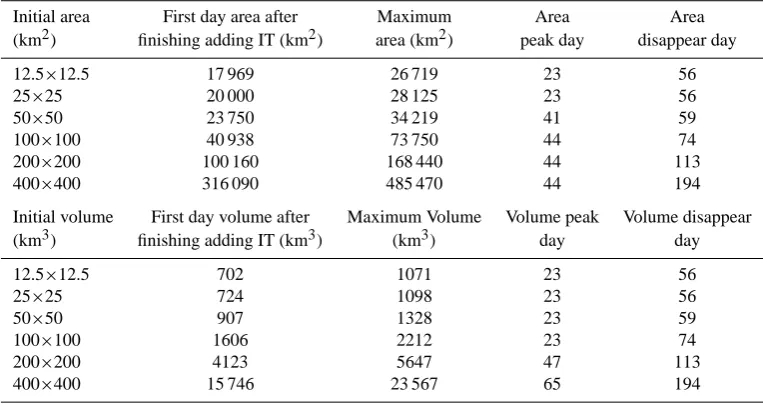
Table 1. Modeled results for the six experiments conducted in this study (Maximum area is the largest area each patch can occupy, Area peak day is the day at which the patch reach its maximum area, and the Area disappear day is the day at which IT concentration becomes lower than 0.3 µmol m−3within that region).
Initial area First day area after Maximum Area Area (km2) finishing adding IT (km2) area (km2) peak day disappear day
12.5×12.5 17 969 26 719 23 56
25×25 20 000 28 125 23 56
50×50 23 750 34 219 41 59
100×100 40 938 73 750 44 74
200×200 100 160 168 440 44 113 400×400 316 090 485 470 44 194
Initial volume First day volume after Maximum Volume Volume peak Volume disappear (km3) finishing adding IT (km3) (km3) day day
12.5×12.5 702 1071 23 56
25×25 724 1098 23 56
50×50 907 1328 23 59
100×100 1606 2212 23 74
200×200 4123 5647 47 113
400×400 15 746 23 567 65 194
whereC is the IT concentration (µmol m−3),N is the total amount of tracer within the patch. Thexis the major axis of the ellipse whileyis the minor axis. Theσx(t),σy(t) are the
standard deviations of the distribution in thex andy direc-tions, respectively. After an initial adjustment, strain and di-lution rates of the surface IT patch were then calculated from the changes in the dimensions of the Gaussian ellipse, by us-ing nonlinear fittus-ing procedure (see methods below, Abraham et al., 2000).
3 Results and discussion
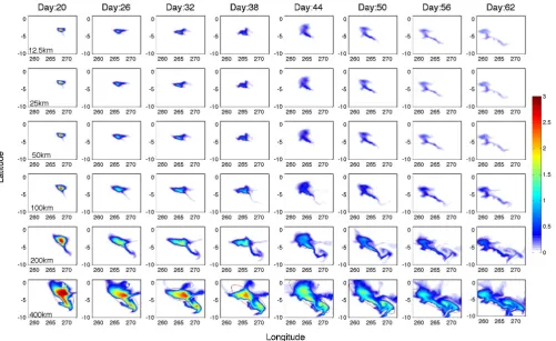
The modeled surface patch follows a similar pattern regard-less of the initial patch size, generally moves cyclonically with its center moving toward the northwest direction dur-ing the first 60 days of the simulation (Fig. 1). The lateral dispersion is largely determined by stirring associated with eddies (Garrett, 1983; Abraham et al., 2000), which changes from an initial square area to a narrow filament. For exam-ple, the initial 12.5×12.5 km patch by day 38 evolves into a filament with a length of 225.2 km, a width of 126.3 km and the resultant eccentricity of 0.83; at the same time, the initial 400×400 km patch turns into a narrow filament with a length of 1865.7 km, a width of 375.4 km and a much higher ec-centricity of 0.98. During the modeled experiments, smaller patches tend to have lower IT concentration and disappear much faster than larger patches (Table 1). The “disappearing day” in Table 1 is the day when IT concentration everywhere within the model domain becomes lower than 0.3 µmol m−3, though at some days Gaussian ellipse fit could not be
ap-plied mainly due to the patch being too small. 12.5×12.5 km patch starts with a surface area of 17 969 km2, reaches its maximum of 26 719 km2that is 48.7% larger at day 23, and disappears at day 56. The volume of 12.5×12.5 km patch follows a similar manner, reaches its maximum of 1071 km3 that is 52.6% larger than first day volume, and disappears at day 56. For surface area, the ratio of maximum to the first day value is 1.67 for large patches (mean value of 100×100, 200×200 and 400×400 patches), which is higher than 1.44 for small patches (mean value of 12.5×12.5, 25×25 and 50×50 patches). While for total volume, the ratio is 1.40 for large patches, which is a little lower than 1.50 for small patches.
Fig. 1. Temporal and spatial variations of the modeled surface IT patch (unit: µmol m−3), only controlled by circulation and diffusion processes. There are six different initial size patches in the experiments, and the area are 12.5×12.5, 25×25, 50×50, 100×100, 200×200, and 400×400 km2, respectively. Red ellipse curve in each figure is the fitted Gaussian ellipse, derived from the IT concentrations.
entire life history of the patch. Both the 12.5×12.5 km and the 25×25 km patch can last 56 days, the 200×200 km patch persists for about 113 days, which is twice the duration of the 12.5×12.5 km patch, while the 400×400 km patch lasts three times longer (194 days) than the 12.5×12.5 km patch. The disappear day for surface area is the same as that for total volume, indicating the patch mostly exists in the upper water column that is consistent with iron fertilization experiments. Previous studies showed that, in the first few days during the patch expansion, length (major axis, 2σx)of the fitted
Gaussian ellipse is observed to increase exponentially with time in response to the strain rate (γ ), while the width (mi-nor axis, 2σy)of the fitted Gaussian ellipse remains constant,
where the thinning effect of strain controls the widening ten-dency due to diffusion (Abraham et al., 2000; Law et al., 2006). This is usually described as the second stage of the tracer dispersion suggested by Garrett (1983). In this study, the strain rate (γ )is calculated by applying a nonlinear fitting procedure to modeled σx(t) and time (t). During the first
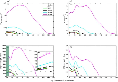
32 days in this modeling study, a robust exponential func-tion is found to fit well to the length data (Fig. 2c). Though the magnitude of ellipse length varies in response to the dif-ferent initial patch sizes, the calculated strain rates are
Fig. 2. Simulated (a) variations of total IT volume, (b) variations of surface area, (c) variations of ellipse length calculated based on the fitted Gaussian ellipse, (d) variations of the ellipse width calculated from fitted Gaussian ellipse, (e) variations of ellipse length during the first 32 days since experiment starts. Solid curves are the exponential regression results for each initial size patch.
ellipse length starts to decrease and width starts to increase for about one week. It is likely caused by the unique, lo-cal physilo-cal conditions because such fluctuation has neither been observed nor modeled before. For the entire life history of the IT patch, variation of length derived from the fitted Gaussian ellipse looks much like a second-order polynomial function with time, which is in a similar manner of varia-tion with surface area and total volume. The width of the ellipse generally decreases with time, though with a small increase around day 41 (Fig. 2d). The standard deviation, however, is much smaller for width variation (e.g. 63 km for 400×400 km patch) than the length data (231 km for 400×400 km patch), which means the width remains rela-tively more constant than the length. For in-situ experiments, previous studies often use either linear or exponential func-tions to model observed variafunc-tions of surface patch. From the model results, however, it is unclear whether the observed surface patch area is an exponential (Law et al., 2006), ex-ponential and linear (Sundermeyer and Price, 1998), or poly-nomial function with time, since that depends on both the observational period and the local physical conditions.
To further investigate how different size patches disperse, we define and calculate the dilution rate (r) of the surface area and total volume as
r=A(t+1t )−A(t )
A(t )∗1t (2)
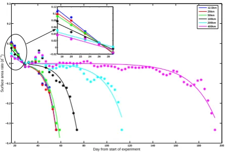
whereAis the area or volume,t is time, and1t is the time interval (Abraham et al., 2000; de Baar et al., 2005). The unit for the dilution rateris day−1. Overall, two stages are found for both the surface area and total volume (Fig. 3 and Fig. 4). In the first stage, the calculated rate decreases linearly with time for about 30 days, which can be expressed as
r=a1t+b1 (3)
20 40 60 80 100 120 140 160 180 200 −0.4 −0.3 −0.2 −0.1 0 0.1 0.2 0.3
Day from start of experiment
Surface area rate (d
−1 ) 12.5km 25km 50km 100km 200km 400km
18 20 22 24 26 28 −0.02 0 0.02 0.04 0.06 0.08 0.1 0.12
Fig. 3. Modeled variations of the dilution rate with time based on the modeled surface tracer area. The modeled data are separated into two stages, the first one is fitted by a linear function, and the second one is fitted by an exponential function.
20 40 60 80 100 120 140 160 180 200 −0.4 −0.3 −0.2 −0.1 0 0.1 0.2 0.3
Day from start of experiment
Volume rate (d
−1 ) 12.5km 25km 50km 100km 200km 400km
18 20 22 24 26 28 −0.04 −0.02 0 0.02 0.04 0.06 0.08 0.1
Fig. 4. Modeled variations of dilution rate with time based on the modeled total tracer volume. The modeled data are separated into two stages, the first one is fitted by a linear function, and the second one is fitted by an exponential function.
have steeper slope (Table 2), which results in less stable ex-panding relative to larger patch.
After 30 days when dilution rate reaches zero, the patch enters its second stage. Smaller patches, such as the 12.5×12.5 km and the 25×25 km, start to decrease much earlier than larger patches (400×400 km). Larger patches can maintain their zero dilution rate for a very long time (e.g. over 100 days for the 400×400 km patch). For the entire second stage, an exponential function is used here to obtain the rate data:
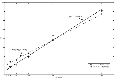
r=a2exp(t /b2) (4) wherea2andb2are the regression coefficients. In this equa-tion, the coefficientb2is the one that controls the duration time in which the patch could maintain its zero dilution rate. The higher the value ofb2, the longer the duration time. Fur-thermore, the value ofb2is also shown to be size-dependent,
which can be estimated well by a linear function of the initial size both for the surface area and total volume data (Fig. 5), implying that a larger initial patch has stronger ability to maintain despite the destruction due to local physical circu-lation and diffusion.
We also conducted the same set of experiments for 2005 at the same location and the same time of the year. Dif-ferent from 2004, the peak time of the surface area for the 400×400 patch is 65 days, which is longer than year 2004 (44 days). Yet, the 12.5×12.5, 25×25, 50×50, 100×100 and 200×200 patches are the same as the year 2004, i.e., 23 days. On the other hand, the disappearing day for 2005 is much longer than for 2004. For example, in the case of the 12.5×12.5 patch, the disappearing day is 86 days for 2005 and 56 days for 2004; for the 200×200 patch it is 155 days for 2005 and 113 days for 2004. It is difficult to generalize the development of different stages with time as described by Garrett (1983), especially using the patch measurements alone. However, the high-resolution physical models can provide detailed information about evaluation of patch dy-namics, especially for different regions and/or year-to-year variations. Two similar stages of linear and exponential rela-tionship for the dilution rate are also found for 2005, which are similar to 2004 in terms of timing in switching between these two stages. The linear relationship exists during the first 38 days, still with steeper slope for smaller initial size patch. The b2 values from exponential regression are also found to be correlated linearly with the initial patch size (see Fig. 5 for the 2004 case), implying that the relationship be-tween dilution rate and initial patch size is independent of the modelling time, though the magnitudes in 2005 case are slightly different from the 2004 case. The longer switching time for 2005 than 2004 implies the patches in 2004 expand much faster than 2005. As a result, patches in 2005 simula-tions have much longer duration in which patch maintains its zero dilution rate. The difference between these two cases is probably caused by the different physical environment, such as surface wind, current, and diffusion effect, as well as some small-scale processes like waves and turbulence that are missed by our physical model. These results again show that local physical conditions are important factors affecting patch dispersal and movement.
Table 2. Coefficients of the regression analysis between dilution rate and time for both surface area and total volume data. During the first 30 days, a linear equation is used, and 30 days later, an exponential equation is used (see Eqs. 3 and 4).
Surface area 12.5 km 25 km 50 km 100 km 200 km 400 km
a1 −0.011 −0.010 −0.009 −0.007 −0.004 −0.004
b1 0.296 0.269 0.244 0.181 0.107 0.105
a2 −1.3×10⁻⁴ −2.2×10⁻⁴ −2.4×10⁻⁴ −1.9×10⁻⁴ −1.2×10⁻⁴ −1.8×10⁻⁵
b2 7.16 7.63 8.03 9.89 14.66 20.11
Total volume 12.5 km 25 km 50 km 100 km 200 km 400 km
a1 −0.007 −0.006 −0.006 −0.005 −0.003 −0.003
b1 0.208 0.183 0.163 0.139 0.084 0.088
a2 −3.8×10⁻⁴ −6.2×10⁻⁴ −6.0×10⁻⁴ −3.3×10⁻⁴ −7.1×10⁻⁵ −1.4×10⁻⁵
b2 8.26 8.88 9.19 10.69 13.65 19.49
12.5 25 50 100 200 400
6 8 10 12 14 16 18 20 22
Size (km)
b2
y=0.034x+6.72
y=0.029x+7.91
Surface area Total volume
Fig. 5. Linear relationship betweenb2, derived from the exponential function fit, and the initial patch size for both the surface area and total volume.
dilution effect is more pronounced in the smaller patches than the larger ones. In addition, the larger patches tend to have more nutrients than smaller ones, which could continue to fuel the phytoplankton growth. As a result, with the same duration of iron fertilization, the larger patches could pro-duce broader spatial extent and longer lasting phytoplankton bloom. Bowie et al. (2001) identified that patch dilution is a major pathway for the decline of added dissolved iron during their experiments. Law et al. (2006) demonstrated that dilu-tion rate has potential impact on the onset of phytoplankton bloom termination and export. The model results indicate that physical dilution rate is not a constant but varies with time. It is largely related to the initial patch size. We spec-ulate that initial patch size can affect patch dilution directly, which has impact on the fate of added iron in the iron enrich-ment experienrich-ments, could further influence the biogeochemi-cal dynamics inside the patch.
In summary, this study shows that in order to study long-term effects of iron fertilization on phytoplankton dynamics and carbon cycle, one must consider the initial patch size as an important factor that controls the outcome of experiments. The larger size of an initial patch tends to have smaller di-lution rate, which in turn increases its ability to maintain high iron concentration inside the patch. The modeled di-lution rate is very sensitive to the initial size. The total vol-ume of materials injected and local physical conditions also play a role in determining the evolution of patch dynamics and its impact on ecosystems and carbon cycling. For ocean iron fertilization experiments, besides the size of initial iron patch and total iron injected, repeatedly adding iron to the same patch of water can also maintain high iron concentra-tion, therefore creating long lasting effects. Modeled results provide important information that can guide large-scale iron fertilization experiments. We understand that only physical processes are included in this study, however, biogeochemi-cal processes may change the behavior of patch dilution sig-nificantly (Neufeld et al., 2002; Elliott and Chu, 2003). De-tailed field measurements and long-term monitoring, includ-ing ecosystem responses to iron fertilization and the fate of fixed carbon, would improve modeling capability and allow us to assess the efficacy of sequestrating atmospheric CO2to the deep sea.
Acknowledgements. We thank Yi Chao at JPL/NASA for sharing
the ROMS circulation model configuration for the Pacific Ocean, and Lei Shi at the University of Maine for designing and setting up the tracer experiments.
References
Abraham, E. R., Law, C. S., Boyd, P. W., Lavender, S. J., Mal-donado, M. T., and Bowie, A. R.: Importance of stirring in the development of an iron-fertilized phytoplankton bloom, Nature, 407, 727–730, 2000.
Bowie, A. R., Maldonado, M. T., Frew, R. D., Croot, P. L., Achter-berg, E. P., Mantoura, R. F. C., Worsfold, P. J., Law, C. S., and Boyd, P. W.: The fate of added iron during a mesoscale fertilisa-tion experiment in the Southern Ocean, Deep-Sea Res. Pt. II, 48, 2703–2743, 2001.
Boyd, P. W., Watson, A. J., Law, C. S., Abraham, E. R., Trull, T., Murdoch, R., Bakker, D. C. E., Bowie, A. R., Buesseler, K. O., Chang, H., Charette, M., Croot, P., Downing, K., Frew, R., Gall, M., Hadfield, M., Hall, J., Harvey, M., Jameson, G., LaRoche, J., Liddicoat, M., Ling, R., Maldonado, M. T., McKay, R. M., Nobber, S., Pickmere, S., Pridmore, R., Rintoul, S., Safi, K., Sut-ton, P., Strzepek, R., Tanneberger, K., Turner, S., Waite, A., and Zeldis, J.: Phytoplankton bloom upon mesoscale iron fertiliza-tion of polar Southern Ocean water, Nature, 407, 695–702, 2000. Boyd, P. W., Law, C. S., Wong, C. S., Nojiri, Y., Tsuda, A., Lev-asseur, M., Takeda, S., Rivkin, R., Harrison, P. J., Strzepek, R., Gower, J., McKay, R. M., Abraham, E., Arychuk, M., Barwell-Clarke, J., Crawford, W., Crawford, D., Hale, M., Harada, K., Johnson, K., Kiyosawa, H., Kudo, I., Marchetti, A., Miller, W., Needoba, J., Nishioka, J., Ogawa, H., Page, J., Robert, M., Saito, H., Sastri, A., Sherry, N., Soutar, T., Sutherland, N., Taira, Y., Whitney, F., Wong, S. K. E., and Yoshimura, T.: The decline and fate of an iron-induced subarctic phytoplankton bloom, Nature, 428, 549–553, 2004.
Boyd, P. W., Jickells, T., Law, C. S., Blain, S., Boyle, E. A., Bues-seler, K. O., Coale, K. H., Cullen, J. J., de Baar, H. J. W., Fol-lows, M., Harvey, M., Lancelot, C., Levasseur, M., Owens, N. P. J., Pollard, R., Rivikin, R. B., Sarmiento, J., Schoemann, V., Smetacek, V., Takeda, S., Tsuda, A., Turner, S., and Watson, A. J.: Mesoscale iron enrichment experiments 1993–2005: Synthe-sis and future directions, Science, 315, 612–617, 2007.
Buesseler, K. O. and Boyd, P. W.: Will ocean fertilization work? Nature., 300, 67–68, 2003.
Buesseler, K. O., Doney, S. C., Karl, D. M., Boyd, P. W., Caldeira, K., Chai, F., Coale, K. H., de Baar, H. J. W., Falkowski, P. G., Johnson, K. S., Lampitt, R. S., Michaels, A. F., Naqvi, S. W. A., Smetacek, V., Takeda, S., and Watson, A. J.: Ocean iron fertilization-Moving forward in a sea of uncertainty, Science, 319, 162, 2008.
Chai, F., Dugdale, R. C., Peng, T. H., Wilkerson, F. P., and Bar-ber, R. T.: One dimensional ecosystem model of the Equatorial Pacific upwelling system, Part I: Model development and silicon and nitrogen cycle, Deep-Sea Res. Pt. II, 49, 2713–2745, 2002. Chai, F., Jiang, M., Chao, Y., Dugdale, R. C., Chavez, F.,
and Barber, R. T.: Modeling responses of diatom productiv-ity and biogenic silica export to iron enrichment in the equato-rial Pacific Ocean, Global Biogeochem. Cy., 21, GB3S90, doi: 10.1029/2006GB002804, 2007.
Chai, F., Liu, G., Xue, H., Shi, L., Chao, Y., Tseng, C. M., Chou, W. C., and Liu, K. K.: Seasonal and interannual vari-ability of carbon cycle in South China Sea: a three dimensional physical-biogeochemical modeling study, J. Oceanogr., 65, 703– 720, 2009.
Coale, K. H., Johnson, K. S., Fitzwater, S. E., Gordon, R. M.,
Tanner, S., Chavez, F. P., Ferioli, L., Sakamoto, C., Rogers, P., Millero, F., Steinberg, P., Nightingale, P., Cooper, D., Cochlan, W. P., Landry, M. R., Constantinou, J., Rollwagen, G., Trasvina, A., and Kudela, R.: A massive phytoplankton bloom induced by an ecosystem-scale iron fertilisation experiment in the equatorial Pacific Ocean, Nature, 383, 495–501, 1996.
Coale, K. H., Johnson, K. S., Chavez, F. P., Buesseler, K. O., Bar-ber, R. T., Brzezinski, M. A., Cochlan, W. P., Millero, F. J., Falkowski, P. G., Bauer, J. E., Wanninkhof, R. H., Kudela, R. M., Altabet, M. A., Hales, B. E., Takahashi, T., Landry, M. R., Bidigare, R. R., Wang, X., Chase, Z., Strutton, P. G., Friederich, G. E., Gorbunov, M. Y., Lance, V. P., Hilting, A. K., Hiscock, M. R., Demarest, M., Hiscock, W. T., Sullivan, K. F., Tanner, S. J., Gordon, R. M., Hunter, C. N., Elrod, V. A., Fitzwater, S. E., Jones, J. L., Tozzi, S., Koblizek, M., Roberts, A. E., Herndon, J., Brewster, J., Ladizinsky, N., Smith, G., Cooper, D., Timothy, D., Brown, S. L., Selph, K. E., Sheridan, C. C., Twining, B. S., and Johnson, Z. I.: Southern Ocean iron enrichment experiment: car-bon cycling in high- and low-Si water, Science, 304, 408–414, 2004.
de Baar, H. J. W., Boyd, P. W., Coale, K. H., Landry, M. R., Tsuda, A., Assmy, P., Bakker, D. C. E., Bozec, Y., Barber, R. T., Brzeinski, M. A., Buesseler, K. O., Boy´e, M., Croot, P. L., Gervais, F., Gorbunov, M. Y., Harrison, P. J., Hiscock, W. T., Laan, P., Lancelot, C., Law., C. S., Levasseur, M., Marchetti, A., Millero, F. J., Nishioka, J., Nojiri, Y., van Oijen, T., Riebe-sell, U., Rijkenberg, M. J. A., Saito, H., Takeda, S., Timmer-mans, K. R., Veldhuis, M. J. W., Waite, A. M., and Wong, C. S.: Synthesis of iron fertilization experiments: From the iron age in the age of enlightenment, J. Geophys. Res., 110, C09S16, doi:10.1029/2004JC002601, 2005.
Elliott, S. and Chu, S.: Comment on “Ocean fertilization ex-periments may initiate a large scale phytoplankton bloom” by Z. Neufeld et al., Geophys. Res. Lett., 30(6), 1274, doi:10.1029/2002GL016255, 2003.
Fujii, M., Yoshie, N., Yamanka, Y., and Chai, F.: Simulated biogeo-chemical responses to iron enrichments in three high nutrient, low chlorophyll (HNLC) regions, Prog. Oceanogr., 64, 307–324, 2005.
Garrett, C.: On the initial streakiness of a dispersing tracer in two-and three-dimensional turbulence, Dyn. Atmos. Oceans., 7, 265– 277, 1983.
Gnanadesikan, A., Sarmiento, J. L., and Slater, R. D.: Effects of patchy ocean fertilization on atmospheric carbon dioxide and biological productivity, Global Biogeochem. Cy., 17(2), 1050, doi:10.1029/2002GB001940, 2003.
Gordon, R. M., Coale, K. H., and Johnson, K. S.: Iron distribu-tions in the Equatorial Pacific: Implicadistribu-tions for new production, Limnol. Oceangr., 42, 419–431, 1997.
Jiang, M. and Chai, F.: Iron and silicate regulation on new and export production in the equatorial Pacific: A physical-biological model study, Geophys. Res. Lett., 31, L07307, doi:10.1029/2003GL018598, 2004.
Jin, X., Gruber, N., Frenzel, H., Doney, S. C., and McWilliams, J. C.: The impact on atmospheric CO2of iron fertilization induced changes in the ocean’s biological pump, Biogeosciences, 5, 385– 406, 2008,
http://www.biogeosciences.net/5/385/2008/.
Gandin, L., Iredell, M., Saha, S., White, G., Woollen, J., Zhu, Y., Chelliah, M., Ebisuzaki, W., Higgins, W., Janowiak, J., Mo, K. C., Ropelewski, C., Wang, J., Jenne, R., and Joseph, D.: The NCEP/NCAR 40-year reanalysis project, Bull. Am. Meteor. Soc., 77, 437–471, 1996.
Kaupp, L., Measures, C., Selph, K., Mackenzie, F.: The distribu-tion of dissolved Fe and Al in the upper waters of the eastern equatorial Pacific. Deep Sea-Res. Pt. II, in press, 2010.
Large, W. G. and Pond, S.: Sensible and latent heat flux measure-ments over the ocean, J. Phys. Oceanogr., 12, 464–482, 1982. Large, W. G., McWilliams, J. C., and Doney, S. C.: Oceanic
verti-cal mixing: A review and a model with nonloverti-cal boundary layer parameterization, Rev. Geophys., 32, 363–403. 1994.
Law, C. S., Watson, A. J., Liddicoat, M. I., and Stanton, T.: Sul-phur hexafluoride as a tracer of biogeochemical and physical processes in an open-ocean iron fertilisation experiment, Deep Sea-Res. Pt. II, 45, 977–994, 1998.
Law, C. S., Crawford, W. R., Smith, M. J., Boyd, P. W., Wong, C. S., Nojiri, Y., Robert, M., Abraham, E. R., Johnson, W. K., Fors-land, V., and Arychuk, M.: Patch evolution and the biogeochem-ical impact of entrainment during an iron fertilisation experiment in the sub-Arctic Pacific, Deep Sea-Res. Pt. II, 53, 2012–2033, 2006.
Ledwell, J. R., Watson, A. J., and Law, C. S.: Mixing of a tracer in the pycnocline, J. Geophys. Res., 103, 21499–21529, 1998. Liu, G. and Chai, F.: Seasonal and interannual variability of
pri-mary and export production in the South China Sea: a three-dimensional physical–biogeochemical model study, ICES J. Ma-rine Syst., 66, 420–431, 2009.
Martin, J. H.: Glacial-interglacial CO2change: the iron hypothesis, Paleoceanography, 5, 1–13, 1990.
Neufeld, Z., Haynes, P. H., Garc¸on, V., and Sudre, J.: Ocean fertilization experiments may initiate a large scale phytoplankton bloom, Geophys. Res. Lett., 29(11), 1534, doi:10.1029/2001GL013677, 2002.
Sundermeyer, M. A. and Price, J. F.: Lateral mixing and the north Atlantic tracer release experiment: observations and numerical simulations of Lagrangian particles and a passive tracer, J. Geo-phys. Res., 103, 21481–21497, 1998.
Timonthy, D. A., Wong, C. S., Nojiri, Y., Ianson, D. C., and Whit-ney, F. A.: The effects of patch expansion on budgets of C,N and Si for the Subarctic Ecosystem Response to Iron Enrichment Study (SERIES), Deep Sea-Res. Pt. II, 53, 2034–2052, 2006. Tsuda, A., Takeda, S., Saito, H., Nishioka, J., Nojiri, Y., Kudo,
I., Kiyosawa, H., Shiomoto, A., Imai, K., Ono, T., Shimamoto, A., Tsumune, D., Yoshimura, T., Aono, T., Hinuma, A., Kinu-gasa, M., Suzuki, K., Sohrin, Y., Noiri, Y., Tani, H., Deguchi, Y., Tsurushima, N., Ogawa, H., Fukami, K., Kuma, K., and Saino, T.: A mesoscale iron enrichment in the western subarctic Pacific induces a large centric diatom bloom, Science, 300, 958–961, 2003.
Wang, X. and Chao, Y.: Simulated sea surface salinity variabil-ity in the tropical Pacific, Geophys. Res. Lett., 31, L02302, doi:10.1029/2003GLD18146, 2004.