https://doi.org/10.5194/tc-12-2005-2018
© Author(s) 2018. This work is distributed under the Creative Commons Attribution 4.0 License.
Medium-range predictability of early summer sea ice thickness
distribution in the East Siberian Sea based on the TOPAZ4
ice–ocean data assimilation system
Takuya Nakanowatari1, Jun Inoue1, Kazutoshi Sato1,a, Laurent Bertino2, Jiping Xie2, Mio Matsueda3, Akio Yamagami3, Takeshi Sugimura1, Hironori Yabuki1, and Natsuhiko Otsuka4
1National Institute of Polar Research, 10-3, Midori-cho, Tachikawa-shi, Tokyo, 190-8518, Japan 2Nansen Environmental and Remote Sensing Center, Thormøhlens gate 47, 5006 Bergen, Norway
3Center for Computational Sciences, University of Tsukuba, 1-1-1 Tennodai, Tsukuba, Ibaraki 305-8577, Japan 4Arctic Research Center, Hokkaido University, Kita-21 Nishi-11 Kita-ku, Sapporo, 001-0021, Japan
apresent address: Kitami Institute of Technology, Kitami, 090-8507, Japan
Correspondence:Takuya Nakanowatari ([email protected]) Received: 30 January 2018 – Discussion started: 1 February 2018
Revised: 9 May 2018 – Accepted: 10 May 2018 – Published: 15 June 2018
Abstract. Accelerated retreat of Arctic Ocean summertime sea ice has focused attention on the potential use of the Northern Sea Route (NSR), for which sea ice thickness (SIT) information is crucial for safe maritime navigation. This study evaluated the medium-range (lead time below 10 days) forecast of SIT distribution in the East Siberian Sea (ESS) in early summer (June–July) based on the TOPAZ4 ice– ocean data assimilation system. A comparison of the oper-ational model SIT data with reliable SIT estimates (hind-cast, satellite and in situ data) showed that the TOPAZ4 reanalysis qualitatively reproduces the tongue-like distribu-tion of SIT in ESS in early summer and the seasonal vari-ations. Pattern correlation analysis of the SIT forecast data over 3 years (2014–2016) reveals that the early summer SIT distribution is accurately predicted for a lead time of up to 3 days, but that the prediction accuracy drops abruptly af-ter the fourth day, which is related to a dynamical process controlled by synoptic-scale atmospheric fluctuations. For longer lead times (>4 days), the thermodynamic melting process takes over, which contributes to most of the remain-ing prediction accuracy. In July 2014, durremain-ing which an ice-blocking incident occurred, relatively thick SIT (∼150 cm) was simulated over the ESS, which is consistent with the re-duction in vessel speed. These results suggest that TOPAZ4 sea ice information has great potential for practical applica-tions in summertime maritime navigation via the NSR.
1 Introduction
During recent decades, sea ice cover in the Northern Hemi-sphere has shown remarkable reduction, and the largest rates of decrease of 100 000 km2decade−1have been observed in
the western Arctic Ocean in summer (Cavalieri and Parkin-son, 2008). Sea ice retreat influences the light conditions for phytoplankton photosynthesis activity (Wassmann, 2011), and the resultant meltwater influences the marine environ-ment via ocean acidification (Yamamoto-Kawai et al., 2011). In winter, shrinkage of the sea ice area in marginal seas such as the Barents Sea changes the surface boundary conditions of the atmosphere, influences planetary waves and causes blocking events, which are one of the possible causes of the recent severe winters in midlatitude regions (Honda et al., 2009; Inoue et al., 2012; Mori et al., 2014; Overland et al., 2015; Petoukhov and Semenov, 2010; Screen, 2017).
Coupled Model Intercomparison Project Phase 5 (CMIP5) global climate model simulation. Currently, the summertime use of the NSR by commercial vessels such as cargo ships and tankers has increased (Eguíluz et al., 2016). Therefore, obtaining precise information on sea ice conditions and eval-uating the forecast of operational sea ice models have be-come urgent issues.
Many previous studies have examined the predictability of summertime sea ice change in the Arctic Ocean in terms of its coverage (Wang et al., 2013) and motion (Schweiger and Zhang, 2015). Kimura et al. (2013) reported a positive correlation in the spatial distribution of summertime sea ice concentration (SIC) with winter ice divergence/convergence. Their study indicated that sea ice thickness (SIT) or sea ice volume before the melt season is a source of predictability for summertime SIC. Recently, their study was supported by hindcast experiments undertaken using a climate model, in which the SIC in the East Siberian Sea (ESS) was shown to have significant seasonal prediction accuracy (Bushuk et al., 2017). The significant impacts of SIT conditions on the seasonal prediction of SIC in the Arctic Ocean have been highlighted by many studies (Lindsay et al., 2008; Holland et al., 2011; Blanchard-Wrigglesworth and Bitz, 2014; Col-low et al., 2015; Melia et al., 2015, 2017; Chen et al., 2017). Thus, the persistence of SIT or sea ice volume is one of the key factors determining the accuracy of seasonal predictions of summertime sea ice area.
Earlier studies have focused primarily on the seasonal to interannual predictability of SIC or sea ice area in the Arctic Ocean; thus subseasonal variation in SIT and its predictabil-ity have not been examined fully for near-term route plan-ning. Although the summertime sea ice extent has rapidly decreased on an interannual timescale, a substantial area of sea ice still remains in critical stretches of the NSR, such as the ESS in early summer (June–July). Since precise informa-tion regarding SIT and its near-future condiinforma-tion is crucial for icebreaker operations (Tan et al., 2013; Pastusiak, 2016), it is important to clarify the medium-range (3 to 10 days lead time) predictability of summertime SIT in the Arctic Ocean. Synoptic-scale fluctuations of cyclone and anticyclone are greater over the Arctic Ocean and Eurasia in summer than in winter (Serreze and Barry, 1988; Serreze and Barrett, 2008). In recent years, there is a risk that an Arctic cyclone be-comes extremely developed and covers the entire Pacific sec-tor (Simmonds and Rudeva, 2012; Yamagami et al., 2017). Because the ESS corresponds to the route of Arctic cyclones generated over the Eurasian continent (Orsolini and Sorte-berg, 2009), it is expected that synoptic-scale atmospheric fluctuations would substantially influence the spatial distri-butions of SIT and ice motion in the ESS. Ono et al. (2016) highlighted the importance of atmospheric prediction accu-racy on medium-range forecasts of sea ice distribution in the ESS based on a case of an extreme cyclone that occurred on 6 August 2012. Mohammadi-Aragh et al. (2018) suggest that the chaotic behaviour of atmospheric prediction
accu-racy controls the short-term predictability of sea ice defor-mation in the Arctic Ocean. On the other hand, earlier studies pointed out that the sea ice melting process is important for the long-term prediction of summertime sea ice extent (e.g. Bushuk et al., 2017). However, the relative importance of dy-namical and thermodynamic processes on the medium-range forecast of summertime sea ice properties has not yet been well understood.
Since 2010, ice–ocean forecasts and a 20-year reanaly-sis are available for the Arctic Ocean, based on the TOPAZ ocean data assimilation system (Towards an Operational Prediction system for the North Atlantic European coastal Zones) in its fourth version (Sakov et al., 2012). The Norwegian Meteorological Institute provides 10-day fore-cast products in daily mean fields, forced at the surface by the European Centre for Medium-Range Weather Fore-casts (ECMWF) operational atmospheric foreFore-casts (Pers-son, 2011), updated daily and distributed by the Coperni-cus Marine Environment Monitoring Services (Simonsen et al., 2017). The reliability of the corresponding TOPAZ4 re-analysis data has been evaluated previously through compar-ison with in situ and satellite SIT data (Xie et al., 2017). They showed that the SIT in the TOPAZ4 reanalysis data is compa-rable to observed values over the Beaufort Gyre and central Arctic Ocean, although the SIT overall shows a negative bias of several dozen centimetres throughout a year. Thus, it is ex-pected that the SIT data in the TOPAZ reanalysis data should also be reliable in the ESS, even in the melting season, and the forecast SIT data should show the prediction accuracy on a medium-range timescale.
In this study, we examined the predictability of the early summer SIT distribution in the ESS on the medium-range timescale and discussed its underlying physical mechanisms, based on the TOPAZ4 forecast data set and trivial dynam-ical and thermodynamdynam-ical models. Section 2 describes the data and methods. Section 3 evaluates the reliability of the SIT data in the TOPAZ4 reanalysis data through comparison with all available in situ and satellite observations, as well as operational model analyses, with particular emphasis on the ESS. In Sect. 4, we examine the predictability of the SIT distribution in the ESS based on TOPAZ4 forecast data. Sec-tion 5 examines the relaSec-tionship between sea ice condiSec-tions and vessel speed during an ice-blocking event that occurred in July 2014. A discussion and the derived conclusions are presented in Sect. 6.
2 Data and methods
reanalysis (Simonsen et al., 2017). The TOPAZ4 system was designed as a regional ice–ocean coupled system forced with atmospheric flux data. The ocean model of TOPAZ4 is based on version 2.2 of the HYCOM model, which uses isopycni-cal vertiisopycni-cal coordinates in the ocean interior andzlevel co-ordinates in the near-surface layer. The sea ice model uses an elastic–viscous–plastic rheology (Hunke and Dukowicz, 1997). The thermodynamic processes are based on a three-layer thermodynamic model with one snow and two ice lay-ers (Semtner, 1976) with a modification for subgrid-scale ice thickness heterogeneities (Fichefet and Maqueda, 1997). The model domain covers the Arctic Ocean and the North At-lantic, and the lateral boundaries are relaxed to monthly mean climatological data. The spatial resolution is 12–16 km with 28 hybrid layers, which constitutes eddy-permitting resolu-tion in low latitude and midlatitude regions but not in the Arctic Ocean. In this system, in situ hydrographic obser-vations are assimilated together with satellite obserobser-vations of the ocean such as sea surface temperature and sea level anomaly. Since this system assimilates the SIC and sea ice velocity (but the latter only in cold season), one should ex-pect adequate simulation of SIT through the ridging process (Stark et al., 2008). It has been reported that the SIT of the TOPAZ4 reanalysis data has substantial negative bias from 2001 to 2010 due to excessive snowfall, which has been mod-ified after 2011 (Xie et al., 2017). Therefore, this study used SIT data from 1 January 2011 to 31 December 2014.
The data assimilation method of TOPAZ4 is a determinis-tic version of the ensemble Kalman filter (EnKF) (Sakov and Oke, 2008) with an ensemble of 100 dynamical members. Since EnKFs have time-dependent state error covariances, this method is suitable for data assimilation of anisotropic variables in areas close to the sea ice edge (Lisæter et al., 2003; Sakov et al., 2012). The TOPAZ4 reanalysis data were produced with the 6 h forcing from the ERA-Interim reanalysis (Dee et al., 2011). The surface turbulent heat flux and momentum flux were both calculated using bulk for-mula parameterizations (Kara et al., 2000; Large and Pond, 1981), instead of the ERA-Interim fluxes themselves. The forecast and reanalysis systems have almost the same set-tings and their results are similar during their overlap period (not shown).
To evaluate the prediction accuracy of the TOPAZ4 fore-cast system, we used daily mean sea ice forefore-cast data during three recent years from 2014 to 2016 (Simonsen et al., 2017). A probabilistic 10-member ensemble forecast was performed with the ECMWF medium-range (up to 10 days) atmospheric forecast data updated daily, out of which only the ensem-ble average is used. To produce 10 ensemensem-ble members in the TOPAZ4 forecast system, the ECMWF global atmospheric forecast data as well as several parameters of sea ice model are perturbed by adding a stochastic forcing term (Evensen, 2003). In this study, we excluded the forecast data in July 2014 because of a real-time forecast production incident (the forecasts were in free-running mode then) (Harald Engedahl,
personal communication, 2018). Since the forecast data were only provided weekly before 2016, a total of 150 cases was assembled during the study period. The skill core was quan-tified using pattern correlation coefficients (PCCs), which are used widely in deterministic forecast verification (Bar-nett and Schlesinger, 1987):
PCC=
N P ij=1
fij−fij
aij−aij
s N P ij=1
fij−fij 2
s N P ij=1
aij−aij2
, (1)
wherefij andaij are forecast and analysis sea ice variables. The overbar denotes the average values over the analysed area (see Fig. 1a); thus the PCC reflects the correlation of ob-served and signal anomalies relative to their respective spa-tial means.
To evaluate the reliability of the SIT values in the TOPAZ4 reanalysis data in early summer, we mainly used the Pan-Arctic Ice Ocean Modeling and Assimilation System (PI-OMAS) outputs, which are derived from the coupled ice– ocean modelling and assimilation system based on the Par-allel Ocean Program (POP) and the thickness and enthalpy distribution (TED) sea ice model, forced with NCEP–NCAR reanalysis data (Zhang and Rothrock, 2003). In this data set, SIC and sea surface temperature are assimilated by adoptive nudging, and many studies (Schweiger et al., 2011; Lindsay and Zhang, 2006; Stroeve et al., 2014) have compared PI-OMAS output with observed SIT data and found it to be the most reliable estimate of observed SIT in the Arctic Ocean (Laxon et al., 2013; Wang et al., 2016).
To evaluate the SIT distribution in the ESS, we used the merged product of CryoSat-2 (CS2) and the Soil Mois-ture and Ocean Salinity (SMOS) SIT products (hereafter, CS2SMOS) as alternative SIT data from 2011 to 2014 (Ricker et al., 2017). They were provided by the online sea-ice data platform “http://www.meereisportal.de/” (for details, see Acknowledgements) (Grosfeld et al., 2016). These data are interpolated to 25 km resolution based on optimal inter-polation and they are available from October to April. In gen-eral, CS2 data have large uncertainty in the estimation of SIT of<1 m, while the SMOS relative uncertainties are lowest for very thin ice. Thus, the merged product is – to date – considered the best estimate of the satellite-based SIT dis-tribution in and around the ESS, although it was reported that there is potential negative bias in mixed first-year and multi-year ice regions such as the Beaufort Sea (Ricker et al., 2017).
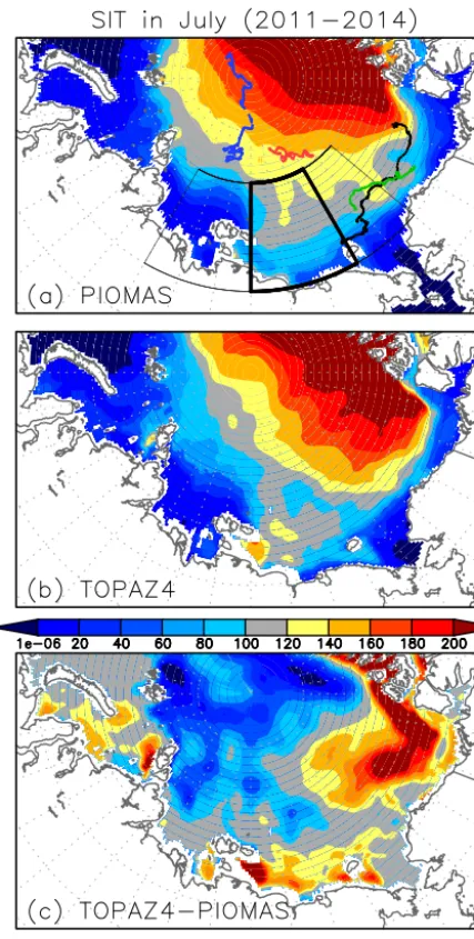
Figure 1. Spatial distribution of climatological monthly mean of SIT (centimetres) in July during 2011–2014: (a) PIOMAS, (b)TOPAZ4 reanalysis and(c)their difference (centimetres). The boundaries of the ESS and Arctic marginal seas are indicated in panel (a)by thick and thin lines. In panel(a), the trajectories of IMB buoys for 2011K, 2012I, 2012J and 2014B (see Table 1 for the details of each buoy data) are shown by black, red, blue and green dots.
with IMB buoy data, we regridded the gridded SIT data along the IMB buoy trajectories. This comparison method is almost identical to that adopted by Sato and Inoue (2018), who com-pared IMB buoy data with SIT data of the NCEP–CFSR re-analysis. Before comparing the gridded SIT data with IMB buoy data in each grid point, we reconstructed these SIT data on a 0.25◦latitude–longitude grid by applying a bilinear in-terpolation. The temporal and horizontal resolutions of the observed and simulated SIT data are summarized in Table 1.
To examine the source of medium-range predictability in the SIT distribution, we also used ECMWF atmospheric forecast data on a 1.25◦latitude–longitude grid from 2013 to 2016, derived from the THORPEX Interactive Grand Global Ensemble through its data portal (http://tigge.ecmwf.int). This data set is very similar to the atmospheric forecast data used in the TOPAZ4 operational forecast system (Simonsen et al., 2017). To examine the atmospheric forecast, we used 51 ensemble daily means of zonal and meridional wind speed at 10 m height on the same days as the TOPAZ4 forecast data at lead times of 0–10 days.
To evaluate the influence of sea ice conditions on vessel speed in the ESS including the Laptev and Kara seas, we used the vessel speed data derived from automatic identifi-cation system (AIS) from two tankers during their passage through the ESS on 4–26 July 2014, which were provided by Shipfinder (http://jp.shipfinder.com/). The temporal reso-lution is about 2 to 3 h, depending on the timing and relative location of the satellite track and the ground-based receiver station of the AIS signal. Their ice classes correspond to IA Super in the Finnish–Swedish ice class rules, and these ves-sels are capable of navigating sea ice regions in which SIT is up to 50–90 cm. Both tankers were likely to be hindered con-siderably by ice conditions, even when escorted by Russian nuclear-powered icebreakers; thus these AIS data are con-sidered suitable for a case study on the influence of SIT on icebreaker speed.
3 Comparisons between TOPAZ4 and other available SIT data
Figure 1a shows the spatial distribution of PIOMAS SIT in July in the Arctic marginal seas of the Laptev Sea, ESS and Chukchi Sea. The PIOMAS shows the tongue-like distribu-tion of SIT, characterized by relatively thick ice (>1.0 m), extending from the North Pole to the ESS. Since in this re-gion, sea ice motion tends to converge during winter (Kimura et al., 2013), the sea ice is likely to increase in thickness by ridging and rafting and thus remains until early the next summer. These features are qualitatively simulated in the TOPAZ4 reanalysis data (Fig. 1b). The PCC of the clima-tological SIT between TOPAZ4 and PIOMAS in the Arctic marginal seas (70–80◦N, 120◦E–160◦W, shown in Fig. 1a) is larger than 0.9 from March to July. The PCCs of the clima-tological SIT between TOPAZ4 and CS2SMOS from March to April are 0.86 and 0.82, which are comparable to those of PIOMAS (Table 2).
reduc-Table 1.List of observed and simulated sea ice thickness data sets.
Data sources Period Spatial resolution Time step
TOPAZ4 Reanalysis 2011–2014 12.5 km Daily Forecast 2014–2016 12.5 km Daily
CS2SMOS 2011–2014 (October–April) ∼25 km 7 days
IMB
2011K 1 September 2011 to 14 May 2012
Pointwise Hourly 2012I 14 August 2012 to 21 December 2012
2012J 25 August 2012 to 3 August 2013
2014B 26 March to 29 July 2014
PIOMAS 2011–2014 ∼0.8◦ Daily
Table 2.Pattern correlations of monthly mean climatologies of SIT in TOPAZ4 with those in PIOMAS and CS2SMOS over the Arctic marginal seas (Laptev, East Siberian and Chukchi seas).
Mar Apr May Jun Jul
PIOMAS 0.92 0.93 0.93 0.92 0.92 CS2SMOS 0.86 0.82 – – –
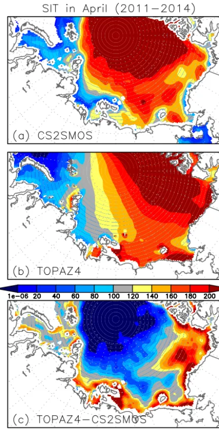
tion in the SIT bias in TOPAZ4 is also found in the compari-son between the TOPAZ4 and CS2SMOS (Table 3). In fact, a similar positive bias emerges in comparison with the climato-logical SIT in CS2SMOS in April (Fig. 2). It should be noted that a larger positive bias in TOPAZ4 is located solely in the region of the Beaufort Gyre, with about 50 cm excess thick-ness (Figs. 1c and 2c). In this region, both SIT data sets show some negative bias relative to the independent SIT estimates derived from US submarine data (Schweiger et al., 2011) and airborne electromagnetic induction (EM) thickness measure-ments (Ricker et al., 2017). This positive bias may be partly related to the underestimation of PIOMAS and CS2SMOS SITs.
Figure 3 shows the time series of daily mean SIT derived from PIOMAS and TOPAZ4 reanalysis and 7-day mean SIT derived from CS2SMOS, averaged over the ESS (70–80◦N, 150–180◦E, shown in Fig. 1a). The TOPAZ4 SIT data are reasonably similar to the seasonal cycle of PIOMAS and CS2SMOS data with maxima in April–May and minima in October–November. In particular, the TOPAZ4 SIT is within the standard deviation of the PIOMAS SIT anomaly in each grid relative to the area-averaged value in early summer (June–July). The monthly mean biases of TOPAZ4 SIT data relative to PIOMAS in June and July are smaller than those from March to May (Table 3). It should be noted that the TOPAZ4 SIT data in 2011 are strongly underestimated in early summer. This might be related to the persistence of the negative bias until 2010 (Xie et al., 2017).
Table 3.Monthly mean biases of TOPAZ4 SIT in the ESS relative to the CS2SMOS and PIOMAS SIT data.
SIT bias (cm) Mar Apr May Jun Jul
CS2SMOS −23 <1 – – – PIOMAS −65 −63 −56 −23 21
In the freezing season, the TOPAZ4 SIT in the ESS tends to be thinner than the PIOMAS SIT and seems comparable to the CS2SMOS SIT. The monthly mean biases of TOPAZ4 SIT relative to CS2SMOS SIT are−23 and<1 cm in March and April, respectively (Table 3). However, we should pay attention to the possibility that the CS2SMOS SIT may be underestimated in this region, because the CS2SMOS greatly depends on the reliability of two merged SIT data, which are CryoSat-2 and SMOS SIT products (Ricker et al., 2017). To check the possibility that the CS2SMOS SIT has a negative bias in this area, we briefly examined the ice type data which were used for the determination of merged SIT products. In the period from 2011 to 2013, the uncertainty of CS2SMOS SIT is out of range for that of PIOMAS, but the CS2SMOS SIT is comparable to that for PIOMAS in 2014 when the sea ice is classified as multi-year ice (Fig. 3). This result implies that the CS2SMOS SIT is underestimated in the ESS due to the large fraction of SMOS SIT products, even in the sea ice thicker than 1 m.
Figure 2. Spatial distribution of climatological monthly mean of SIT (centimetres) in April during 2011–2014: (a)CS2SMOS, (b)TOPAZ4 reanalysis and(c)their difference (centimetres).
the reliability of TOPAZ4 SIT data in the ESS in early sum-mer. Thus, at least the overall spatial distribution of SIT in the ESS is qualitatively simulated in the TOPAZ4 and the in-herent negative bias is suppressed in early summer, which is partly related to the compensation by the positive bias near the shelf region of the ESS.
Years
ESS (70°–80° N, 150°–180° E)
Figure 3.Time series of daily mean SIT (centimetres) averaged over the ESS (rectangular region denoted by black line in Fig. 1a) derived from CS2SMOS (black), TOPAZ4 reanalysis (red) and PI-OMAS (blue) from January 2011 to August 2014. For CS2SMOS data, 7-day mean values are shown. The standard deviations of area-averaged data are shown by vertical lines. The ice types (2: first-year ice, 3: multi-year ice) used for the choice of satellite SIT retrievals in CS2SMOS are shown by green bar. The scale for the ice type is located on the right vertical axis.
0 50 100 150 200 250
0 50 100 150 200 250
IMB
TOPAZ
SIT in and around the ESS (cm)
N = 845 Corr. = 0.96
RMSD = 29.4 Mean bias = 8.6 2011K (Sep−May)
2012I (Aug−Dec) 2012J (Aug−Jun) 2014B (Mar−Jul)
Years
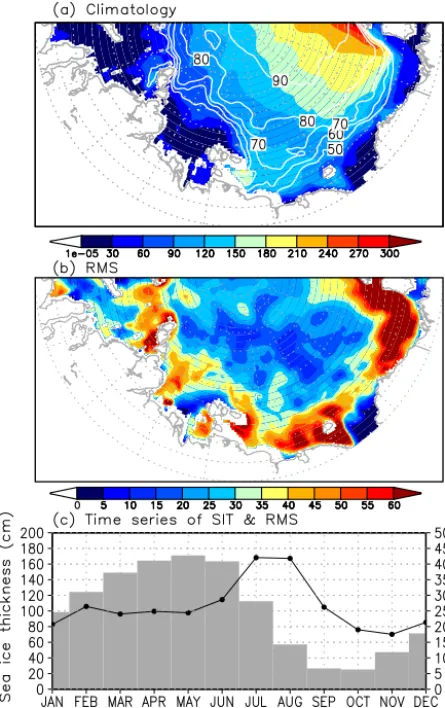
Figure 5. Spatial distribution of(a)monthly mean (colours) cli-matological SIT (m) in the TOPAZ4 reanalysis and (b) the rms variability of daily mean SIT (colours) in July during 2011–2014. The monthly mean of climatological SIC (white contours) in July is indicated in panel(a). The rectangular region enclosing the ESS (70–80◦N, 150–180◦E) is shown in panel(b).(c)Time series of monthly mean SIT (grey shading) and rms of TOPAZ4 reanalysis (black line) averaged over the ESS. The scale of the rms is indi-cated on the right axis.
4 Medium-range forecast of SIT distribution in the ESS
In this section, we evaluate the prediction accuracy of SIT based on the PCCs between the analysis and predicted data in the ESS. However, before this evaluation, we examine the mean fields and the variability of the SIT and SIC tions in early summer. Figure 5a presents the spatial distribu-tions of the climatological SIT and SIC in July, which show that relatively thick sea ice (∼1 m) covers 50–70 % of the ESS. Along the zone of the sea ice edge, the temporal stan-dard deviation of the daily mean SIT anomaly is relatively large with a maximum value of 0.6 m in the coastal region
Figure 6.The prediction accuracy (PCC) of the SIT forecast in the ESS (70–80◦N, 150–180◦E) in each month obtained from(a)an operational forecast model and(b)persistency of the initial value, averaged from 2014 to 2016. The standard deviations of the PCCs are shown with white contours. In panel(c), the fraction of variance explained by operational forecast relative to the persistency (%) is shown by the contour (the region where the fraction is larger than 10 % is shaded).
(Fig. 5b), and the area-averaged value is at maximum in July– August (Fig. 5c). Since the SIT reduction rate in the ESS is strongest in these months (Fig. 5c) and the storm activity is prevalent for periods of several days (Orsolini and Sorteberg, 2009), it is likely that dynamical and thermodynamically in-duced SIT variations are large. Note that the rms of the SIC anomaly averaged over the ESS also shows a similar sea-sonal cycle (not shown). Thus, it is meaningful to examine the medium-range predictability of early summer SIT distri-bution in the ESS.
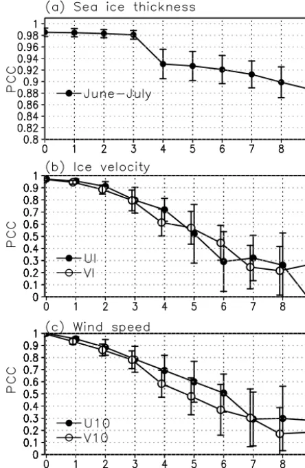
Figure 7.PCCs between forecast and analysis(a)SIT,(b) zonal and meridional ice speed, and(c)zonal and meridional surface wind speed from operational TOPAZ4 data in early summer (June–July) averaged over 2014–2016. Error bar indicates the standard deviation of the PCCs.
SIT (Fig. 6b). The contribution of the operational model on the forecast is less than 5 % at shorter timescales (<3 days) (Fig. 6c), but the contribution of the operational model grad-ually increases at longer lead times except in May and Oc-tober. In July, the contribution of the operational model on the prediction accuracy reaches∼15 % at 7-day lead times. These results indicate that the operational model substan-tially improves the medium-range prediction accuracy of the SIT distribution in summer.
Figure 7a shows the PCC of SIT distribution averaged in early summer (June–July). The SIT distribution is predicted accurately for a lead time of up to 3 days (Fig. 7a); how-ever, the prediction accuracy decreases abruptly at a lead time of 4 days, in which the standard deviation is also rel-atively large. Such an abrupt reduction in the prediction ac-curacy and the enhanced standard deviation are also found in May and September, although the absolute values of the reduction rates are smaller than in July. Since the influence
of sea ice melt is small in these months (Fig. 5c), the abrupt reduction in early summer SIT prediction accuracy might be attributable to dynamical advection of sea ice.
To examine the influence of dynamical processes on the prediction accuracy of early summer SIT distribution, we consider the prediction accuracy of sea ice velocities and surface wind velocities. The prediction accuracy of sea ice velocity stays on a high level (>0.8) with small spread for a lead time of up to 3 days, but decreases down to 0.6–0.7 for a lead time of 4 days (Fig. 7b). The early summer pre-diction accuracy of surface wind speed also shows the same abrupt decrease at a lead time of 4 days, and the rate of de-crease in prediction accuracy is larger in meridional direction (Fig. 7c). Since the SIT distribution has a tongue-like distri-bution (Fig. 5a), it is suggested that the meridional compo-nent of SIT advection is sensitive to the sea ice transport in ice edges, which influences the SIT distribution in the ESS. These results confirm that the prediction accuracy of the sea ice velocities are strongly related to those of surface wind speeds in the ESS.
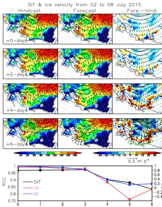
Figure 8 shows the temporal evolutions of SIT and ice ve-locity for analysis and a forecast bulletin starting from 2 July 2015, which is a typical case of the abrupt decrease in the prediction accuracy of SIT as well as sea ice velocities for a lead time of 4 days (Fig. 8; lower panel). For lead times of+0 (2 July) to +2 days (4 July), the spatial distributions of SIT and ice velocity are predicted accurately with only small differences between them (Fig. 8c). At a lead time of
+4 days (6 July), the analysed sea ice velocity is directed northwestward in the ESS, which is related to the cyclonic circulation over the Novosibirsk Islands; however, the pre-dicted sea ice velocity is directed southwestward. At a lead time of+6 days, the predicted and analysed sea ice veloci-ties are largely unrelated. The resultant onshore anomaly of sea ice velocity leads to positive and negative anomalies in SIT in the coastal and offshore regions, respectively. We also examined the time evolutions of the surface wind velocities in the atmospheric forecast data and found them very similar to the sea ice velocity fields (not shown). These results indi-cate that the abrupt reduction in the prediction accuracy of early summer SIT in the ESS is related to a deficiency in the prediction of Arctic cyclone formation.
Further, we examine diagnostically the ice drift speed and direction based on a classical free-drift theory (Leppäranta, 2005), using the sea ice speed of TOPAZ4 reanalysis data and ERA-Interim atmospheric wind data in July 2011–2014. The general solution of sea ice speed (u) can be described as complex numbers:
u=αe−iθUa+Uwg, (2)
whereUaandUwgare the wind speed and geostrophic
(a) (b) (c)
Figure 8.Temporal evolution of SIT (centimetres; colours) and ice velocity (m s−1; vectors) distribution for the(a)analysis,(b)forecast and(c)the difference between the forecast and analysis at increasing lead times from+0 days to+6 days initialized on 2 July 2015. The corresponding PCCs for the SIT (black), zonal (red) and meridional ice speeds (blue) in the ESS (right-lower panel of the time evolution) are shown in the lower panel. The scale for the PCCs of the zonal and meridional ice speeds is indicated on the right axis.
the geostrophic water velocityUwg, the wind factor and
de-viation angle can be obtained in the following form: α4+2 sinθwRNaα3+R2Na2α2−Na4=0, (3) θ=arctan
tanθw+ RNa αcosθw
−θa, (4)
whereθwandθaare the boundary layer turning angles of
wa-ter and air. The turning angleθis the angle between the vec-tors of the ice–water stress and the sea ice motion, which is a consequence of the viscous effect within the ocean boundary layer. The Nansen numberNa is defined by√ρaCa/ρwCw,
whereρaandρwrepresent the densities of air and water, and
Ca andCw are air and water drag coefficients. The Rossby
numberRis defined by(ρhicef ) / (ρwCwNa|Ua|), whereρ
is the ice density,f is the Coriolis parameter, and|Ua|is the
speed of the surface wind. To calculate the wind factorαand the deviation angleθ under a given surface wind speed, we used constant parameters ofCa=1.2×10⁻³,Cw=5×10⁻³, ρa=1.3 kg m−3,ρw=1026 kg m−3,ρ=910 kg m−3, f=
1.3×10⁻⁴s−1andθw=20◦, which are values typical of the
Arctic Ocean (McPhee, 2012). The value ofαwas calculated numerically from a fourth-order polynomial (Eq. 3).
0 2 4 6 8 10 0
0.05 0.1 0.15 0.2 0.25
10−m wind speed (m s )
Ice speed (m s )
(a)
0 2 4 6 8 10
0 10 20 30 40 50 60 70 80 90 100
10−m wind speed (m s )
Wind−ice angle (degree)
(b)
-1
-1
-1
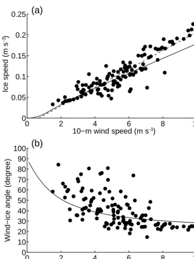
Figure 9. (a) Relationship between 10 m wind speed (m s−1) in the ERA-Interim reanalysis data and sea ice speed (m s−1) in the TOPAZ4 reanalysis averaged over a part of the ESS (72–76◦N, 150–170◦E) during 1–31 July 2011–2014. Broken and solid lines indicate the regression line of ice speed on 10 m wind speed (y=
0.0224x−0.0112) and the theoretical ice speed estimated based on classical free-drift theory.(b)Angle (degrees) of sea ice velocity relative to surface wind vectors averaged over the ESS. Positive val-ues indicate that sea ice drift is to the right of the wind direction. Solid curve indicates the wind–ice velocity angle estimated based on classical free-drift theory.
height) averaged over a part of the ESS (Fig. 9a). The cor-relation between them is 0.96, which is significant at the 99 % confidence level, based on the Monte Carlo simula-tion (Kaplan and Glass, 1995). The regression coefficient of ice speed for the 10 m wind speed is 0.022, which is consis-tent with the well-known 2 % relationship between the speed of ice and the surface wind speed (Thorndike and Colony, 1982). The number of days of the TOPAZ4 ice speed data within ±20 % of the theoretical value is 79, which account for 63 % of the total analysed period. Note that the observed regression coefficient is somewhat larger than the theoreti-cal value (0.018) averaged over the range of surface wind speed of 2–10 m s−1calculated from Eq. (2). Since the clas-sical free-drift theory (Leppäranta, 2005) neglects both the Ekman layer velocity and the ocean geostrophic velocity, the absence of an ice–ocean boundary layer is likely to underesti-mate the wind-induced ice velocity (Park and Stewart, 2016). The deviation angle of sea ice motion in TOPAZ4 is esti-mated as 20–40◦under the wind condition>5 m s−1, but it
gradually increases to 40–70◦under weaker wind conditions of<5 m s−1(Fig. 9b). The decrease in the deviation angle
as the surface wind strengthens is also consistent with ear-lier studies (Thorndike and Colony, 1982). These observed deviation angles are comparable with their theoretical val-ues calculated using Eq. (4). The finding that the estimated values of the wind factor and the deviation angle are approx-imately within the range of typical surface wind parameters (i.e. 2 % for the wind factor and 30◦for the deviation angle) in the Arctic Ocean confirms that sea ice velocity in the ESS is controlled predominantly by wind stress drag; thus the in-fluence of ocean currents is not essential.
It is interesting that the prediction accuracy of SIT in early summer remains at∼0.9 for the PCC core at lead times of more than 4 days (Fig. 7a), despite the poorer prediction ac-curacy of sea ice velocity (Fig. 7b). This suggests that the SIT prediction accuracy after a lead time of 4 days is not strongly attributed to the dynamical process but rather the thermody-namic process (i.e. the melting process of sea ice). To evalu-ate the effect of sea ice melting on SIT prediction accuracy, we roughly estimated the thermodynamic SIT change based on a simple sea ice melting model, as follows:
hp(t )=ha(t0)+1t×dh/dt, (5)
wherehpis the predicted thermodynamic SIT change,hais the initial condition, which is derived from the analysis SIT, and dh/dt is the rate of reduction in SIT due to sea ice melt-ing. It is known that the summertime surface heat flux in the Pacific sector of the Arctic Ocean is dominated by the short-wave radiation flux (Perovich et al., 2007; Steele et al., 2008). Recently, the seasonal evolution of sea ice retreat in early summer has been found to be explained well by a simplified ice–ocean coupled model, in which shortwave radiation is as-sumed constant (Kashiwase et al., 2017). Therefore, for the melting rate of the SIT in each year, we used the reduction rate of SIT calculated from the climatological analysis SIT data during 2013–2016, which is likely to reflect the typi-cal thermodynamic melting rate in recent years and the SIT change due to transient sea ice advection seems to be negli-gible. Here, we also evaluate the prediction accuracy of the persistency in the initial SIT in the ESS (first term of the RHS in Eq. 5).
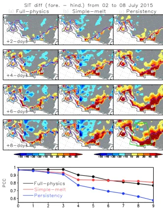
Figure 10.The PCCs between forecast and analysis SIT from the full physics model (black), persistency (red) and a simple melting model (blue) in early summer (June–July) averaged from 2014 to 2016. Error bar indicates the standard deviation of the PCCs.
full physics model is higher than the simple melting and per-sistency models for lead times of 0–5 days but comparable with the prediction accuracy of the simple melting model at longer lead times (>6 days). In the SIT difference map of the full-physics model minus the operational analysis, a positive anomaly (i.e. overestimation of SIT) is evident along the sea ice edge at a lead time of 4 days and then gradually increases to a lead time of 8 days. For the case of the simple melt-ing model, a similar positive anomaly emerges at a lead time of 4 days, but the positive anomaly appears stationary along the coastal region, in contrast to the full physics model. The persistency model overestimates SIT over the entire region during the prediction. These results support the idea that the melting process is important in the prediction of early sum-mer SIT over longer timescales.
5 Case study of ice-blocked incident in the ESS in July 2014
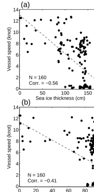
From the perspective of operational application of the TOPAZ4 sea ice data on the maritime navigation of the NSR, we briefly examine the relationship between the sea ice conditions and AIS vessel speed data for the case of an ice-blocking incident involving two vessels based on the TOPAZ4 reanalysis data. Figure 12 shows the vessel tracks during 4–30 July 2014, when the two vessels became blocked in the ESS for about 1 week. During this period, SIT in ex-cess of 100 cm is found in the ESS with a maximum thick-ness of 150 cm. A joint statistical analysis of the daily mean SIT in the TOPAZ4 reanalysis and the vessel speed along the route indicates that vessel speed is significantly anticor-related with SIT (−0.56) during the entire passage (Fig. 13a), which is significant at the 99 % confidence level based on a Monte Carlo technique (Kaplan and Glass, 1995). We also
examined the corresponding SIC data in TOPAZ4 reanalysis data, but the correlation between the vessel speed and SIC is−0.41 (Fig. 13b), which is insignificant at the 99 % con-fidence level. The scatter plots for SIC indicate that the SIC value is partly insensitive to the vessel speed higher than 5 kn. Thus, these results suggest that the vessel speed was influ-enced by sea ice stress due to SIT and indirectly supports the reliability of the daily mean SIT of the TOPAZ4 reanalysis data in the ESS in early summer.
6 Summary and discussion
In this study, the medium-range forecast of early summer SIT distribution in the ESS was evaluated using the TOPAZ4 data assimilation system. Comparisons between the opera-tional model, observations and TOPAZ4 reanalysis SIT data showed that the TOPAZ4 reanalysis qualitatively reproduces the tongue-like distribution of SIT in the ESS in early sum-mer and its seasonal variation (maximum in April–May and minimum in October–November), including the rates of ad-vance and melting of sea ice in the ESS). Although in this region, the inherent negative bias of SIT in TOPAZ4 is rela-tively large in March–May, the bias is reduced in early sum-mer (June–July) within∼ ±20 cm due to the excess of SIT along the coastal region in the ESS. The TOPAZ4 SIT data also correspond well to IMB buoy data in and around the ESS with a mean bias of∼9 cm and a root mean square error of
∼30 cm. Thus, the TOPAZ4 SIT data could be considered to be reliable estimates for the ESS even in the absence of satellite observations in summer.
For the positive bias of the SIT in TOPAZ4 along the coastal region of the ESS, there is a possibility that the SIT estimates (PIOMAS and CS2SMOS) used for the compari-son are themselves underestimated. Schweiger et al. (2011) pointed out that the SIT of PIOMAS is underestimated by
−17 cm in the basin area of the Arctic Ocean, including the Beaufort Sea where the heavily deformed sea ice formation occurs. Also, it was reported that the CS2SMOS SIT data tend to underestimate SIT in regions where multi-year ice and first-year ice are formed, due to the relative accuracy of CryoSat-2 and SMOS and the merging algorithm (Ricker et al., 2017). Since in the ESS, sea ice motion strongly con-verges during winter (Kimura et al., 2013), there is a pos-sibility that the sea ice in the ESS is also heavily deformed in sea ice thicker than 1 m along the coastal region. In fact, our analysis based on the AIS data suggests that SIT in ex-cess of 100 cm is found near the coast of the ESS. Thus, for a precise evaluation of the SIT distribution in the ESS, the further improvement in ice-type as well as denser in situ SIT measurements are needed.
(a) (b) (c)
Figure 11.Temporal evolution of SIT differences (centimetres; colours) between the forecast and analysis data at lead times increasing from
+2 to+8 days, initialized on 2 July 2015. In each panel, the sea ice edge of the analysis, defined by 30 % SIC, is shown. Corresponding PCCs for the full physics model (black), a simple melting model (red) and persistency (blue) in the ESS (right-lower panel of the time evolution) are shown in the lower panel.
large spread, the SIT distribution was predicted accurately for a lead time of up to 3 days, and the prediction accu-racy drops abruptly after the fourth day. A similar change in prediction accuracy was also found for sea ice velocity and surface wind speed over the ESS. Diagnostic analysis of the sea ice velocity variability revealed that the early summer ice speed and direction over the EES could be explained well by the free-drift mechanism with a wind factor of 2.2 % and a deviation angle of 30–50◦. Their results suggested that the large reduction in prediction accuracy could be attributed to the process of dynamical advection of sea ice; thus the pre-diction of early summer SIT distribution will depend on the
How-Figure 12. Trajectory of the two tankers over the ESS based on AIS data. The routes cross the ESS from the Laptev Sea on 4 July 2014 to the port of Yamal on 31 July 2014 via the port of Pevek on 20 July 2014. The forward route is highlighted by green circles. The SIT (centimetres; colours) and SIC (%; contours) averaged over the period of the forward route are shown.
ever, Yamagami et al. (2018) reported that the prediction of Arctic cyclones generated in summer is limited to 4 days, which is shorter than is the case for the midlatitudes (Froude, 2010). As this area is located near the transit zone of summer-time storm tracks generated over Eurasia (Serreze and Barry, 1988), the predictability of Arctic cyclones could be an im-portant factor in the determination of the lead time of sur-face wind speed and thus of the SIT distribution in the ESS. The low prediction accuracy of the meridional wind and ice speed suggested that the meridional component of sea ice ad-vection contributes substantially to the SIT distribution in the ESS. Since it was reported that additional radiosonde obser-vations over the Arctic Ocean have considerable impact on the prediction accuracy in synoptic-scale fluctuations (Inoue et al., 2015; Yamazaki et al., 2015), additional radiosonde observations acquired over the Arctic Ocean could lead to a further extension of the lead time for medium-range forecast of SIT distribution.
Based on sensitivity experiments using a simple melt-ing and a persistency model, it was found that the longer timescale prediction of SIT in early summer could be at-tributed to the thermodynamic melting process. As the short-wave radiation flux is maximum in early summer (June– July), the change in SIT due to the advection in relation to synoptic-scale atmospheric fluctuations is likely to be smaller than the thermodynamic SIT reduction along the sea ice edge. Although the recognition of the importance of the thermodynamic melting process on sea ice prediction on seasonal timescales has been pointed out by earlier stud-ies (Kimura et al., 2013; Bushuk et al., 2017; Kashiwase et al., 2017), our study clarified that the influence has a sub-stantial role on the medium-range forecast of early summer
0 50 100 150
0 2 4 6 8 10 12 14
Sea ice thickness (cm)
Vessel speed (knot)
N = 160 Corr. = −0.56
(a)
0 20 40 60 80 100
0 2 4 6 8 10 12 14
Sea ice concentration (%)
Vessel speed (knot)
N = 160 Corr. = −0.41
(b)
Figure 13.Scatter plots of hourly vessel speeds (knots) and(a)daily mean SIT (centimetres) and(b) SIC (%) in TOPAZ4 reanalysis from 4–30 July 2014. In each panel, the regression line of vessel speed for each variable is shown by a broken line.
SIT distribution. Thus, the influence of sea ice advection on early summer sea ice prediction is limited to a lead time of 4–5 days, but is dominated by the thermodynamic melting process at a later stage of the lead times. In other words, the SIT prediction accuracy in early summer is not necessarily worse at the longer timescale. It is noteworthy that the dy-namical process is not unimportant for long-term prediction in the SIT distribution in early summer, because the predic-tion accuracy at a lead time of 3 days is important as the ini-tial conditions for the melting process dominated for a lead time of more than 4 days. Thus, it is concluded that the at-mospheric prediction accuracy for a lead time of up to 3 days contributes to the short and medium-range estimates of the SIT distribution in early summer.
to be above 150 cm. Statistical analysis suggested that vessel speed was significantly anticorrelated with the daily mean SIT variations (−0.56) rather than the SIC (−0.41). This re-sult demonstrated the reliability of the early summer SIT dis-tribution in the TOPAZ4 reanalysis data and its high potential for operational use in support of maritime navigation of the NSR. However, this result was only based on a case study of two ships in July 2014. To clarify the determinant factor on vessel speed, comprehensive statistical analysis will be needed based on the speed data of different types of vessel.
Future projections for storm track activity (intensity and number) under the scenario of Arctic climate change have been addressed by several researchers. For example, based on control experiments using climate models, Bengtsson et al. (2006) found that summertime storm activity is expected to increase. Orsolini and Sorteberg (2009) found that the number of storms, particularly along the Eurasian Arctic coast, could increase in the future because of the local en-hancement of the meridional temperature gradient between the Arctic Ocean and the warmed Eurasian continent. Nishii et al. (2015) supported their findings based on analyses us-ing the CMIP3 and CMIP5 global climate model simula-tions, although they highlighted that the CMIP projections had considerable uncertainty. Thus, further investigations of the formation and the development mechanisms of summer-time Arctic cyclones are needed for the improvement of the prediction accuracy of atmospheric wind conditions, which are responsible for the forecast of early summer sea ice dis-tribution over 4 days.
Data availability. TOPAZ4 reanalysis and forecast data sets are
available for download at http://marine.copernicus.eu/ (last ac-cess: 29 December 2016). The PIOMAS SIT data are available for download at ftp://pscftp.apl.washington.edu/zhang/PIOMAS/ data/ (last access: 13 January 2017). The CS2SMOS data set is available for download at http://www.meereisportal.de (last ac-cess: 26 May 2016). The IMB buoy data are available at http:// imb-crrel-dartmouth.org/ (last access: 20 June 2017). The ECMWF atmospheric forecast data are available at https://www.ecmwf.int/ en/research/projects/tigge and were made available by Mio Mat-sueda and Akio Yamagami at the University of Tsukuba.
Competing interests. The authors declare that they have no conflict
of interest.
Acknowledgements. The TOPAZ4 reanalysis and forecast data
were provided by Copernicus Marine Environment Monitoring Service (http://marine.copernicus.eu/). The PIOMAS outputs were provided by Jinlun Zhang of University of Washington via FTP site (ftp://pscftp.apl.washington.edu/zhang/PIOMAS/data/). The merging of CryoSat-2 und SMOS data were funded by the ESA project SMOS+ Sea Ice (4000101476/10/NL/CT and 4000112022/14/I-AM) and data from 2010 to 2014 were obtained
from http://www.meereisportal.de (grant no. REKLIM-2013-04). The IMB buoy data were obtained from the Cold Regions Research and Engineering Laboratory of the U.S. Army Engineer Research and Development Center (http://imb-crrel-dartmouth.org/). The ECMWF atmospheric forecast data were provided by the ECMWF TIGGE portal site via the TIGGE medium of the University of Tsukuba (http://gpvjma.ccs.hpcc.jp/TIGGE/). We wish to thank three anonymous reviewers for their constructive comments. The TOPAZ4 forecast data were analysed using the Pan-Okhotsk Infor-mation System of ILTS of Hokkaido University. We thank James Buxton MSc from Edanz Group (www.edanzediting.com./ac) for correcting a draft of this manuscript. Some figures were produced with the GrADS package developed by B. Doty. This work was supported by the Arctic Challenge for Sustainability (ArCS) project of the Ministry of Education, Culture, Sports, Science and Technology in Japan, and JSPS KAKENHI grant numbers 17KK0014, 18H03745.
Edited by: John Yackel
Reviewed by: three anonymous referees
References
Barnett, T. P. and Schlesinger, M. E.: Detecting changes in global climate induced by greenhouse gases, J. Geophys. Res., 92, 14772–14780, https://doi.org/10.1029/JD092iD12p14772, 1987. Bengtsson, L., Hodges, K. I., and Roeckner, E.: Storm Tracks and Climate Change, J. Climate, 19, 3518–3543, https://doi.org/10.1175/JCLI3815.1, 2006.
Blanchard-Wrigglesworth, E. and Bitz, C. M.: Characteristics of Arctic Sea-Ice Thickness Variability in GCMs, J. Climate 27, 8244–8258, 2014.
Bushuk, M., Msadek, R., Winton, M., Vecchi, G. A., Gudgel, R., Rosati, A., and Yang, X.: Skillful regional prediction of Arctic sea ice onseasonal timescales, Geophys. Res. Lett. 44, 4953– 4964, https://doi.org/10.1002/2017GL073155, 2017.
Cavalieri, D. J. and Parkinson, C. L.: Arctic sea ice variabil-ity and trends, 1979–2006, J. Geophys. Res., 113, C07003, https://doi.org/10.1029/2007JC004558, 2008.
Chen, Z., Liu, J., Song, M., Yang, Q., and Xu, S.: Impacts of Assim-ilating Satellite Sea Ice Concentration and Thickness on Arctic Sea Ice Prediction in the NCEP Climate Forecast System, J. Cli-mate, 30, 8429–8446, 2017.
Collow, T., Wang, W., Kumar, A., and Zhang, J.: Improving Arctic Sea Ice Prediction Using PIOMAS Initial Sea Ice Thickness in a Coupled Ocean–Atmosphere Model, Mon. Weather Rev., 143, 4618–4630, https://doi.org/10.1175/MWR-D-15-0097.1, 2015. Dee, D. P., Uppala, S. M., Simmons, A. J., et al.: The
ERA-Interim reanalysis: configuration and performance of the data assimilation system, Q. J. Roy. Meteor. Soc., 137, 553–597, https://doi.org/10.1002/qj.828, 2011.
Eguíluz, V. M., Fernández-Gracia, J., Irigoien, X., and Duarte, C. M.: A quantitative assessment of Arctic shipping in 2010–2014, Sci. Rep., 6, 30682, https://doi.org/10.1038/srep30682, 2016. Evensen, G.: The ensemble Kalman filter: Theoretical
Fichefet, T. and Maqueda, M. A. M.: Sensitivity of a global sea ice model to the treatment of ice thermody-namics and dythermody-namics, J. Geophys. Res., 102, 12609–12646, https://doi.org/10.1029/97JC00480, 1997.
Froude, L. S. R.: TIGGE: Comparison of the prediction of Northern Hemisphere extratropical cyclones by different en-semble prediction systems, Weather Forecast., 25, 819–836, https://doi.org/10.1175/2010WAF2222326.1, 2010.
Grosfeld, K., Treffeisen, R., Asseng, J., Bartsch, A., Bräuer, B., Fritzsch, B., Gerdes, R., Hendricks, S., Hiller, W., Heygster, G., Krumpen, T., Lemke, P., Melsheimer, C., Nicolaus, M., Ricker, R., and Weigelt, M.: Online sea-ice knowledge and data platform, available at: www.meereisportal.de (last access: 26 May 2016), Polarforschung, Bremerhaven, Alfred Wegener Institute for Po-lar and Marine Research and German Society of PoPo-lar Research, 85, 143–155, https://doi.org/10.2312/polfor.2016.011, 2016. Holland, M. M., Bailey, D. A., and Vavrus, S.: Inherent sea ice
predictability in the rapidly changing Arctic environment of the Community Climate System Model, version 3, Clim. Dy-nam., 36, 1239–1253, https://doi.org/10.1007/s00382-010-0792-4, 2011.
Honda, M., Inoue, J., and Yamane, S.: Influence of low Arctic sea-ice minima on anomalously cold Eurasian winters, Geophys. Res. Lett., 36, L08707, https://doi.org/10.1029/2008GL037079, 2009.
Hunke, E. and Dukowicz, J.: An Elastic–Viscous–Plastic Model for Sea Ice Dynamics, J. Phys. Oceanogr., 27, 1849–1867, 1997. Inoue, J., Hori, M., and Takaya, K.: The role of Barents sea ice in
the wintertime cyclone track and emergence of a Warm-Arctic Cold Siberian anomaly, J. Climate, 25, 2561–2568, 2012. Inoue, J., Yamazaki, A., Ono, J., Dethloff, K., Maturilli, M., Neuber,
R., Edwards, P., and Yamaguchi, H.: Additional Arctic observa-tions improve weather and sea-ice forecasts for the Northern Sea Route, Sci. Rep., 5, 16868, https://doi.org/10.1038/srep16868, 2015.
Jung, T. and Matsueda, M.: Verification of global numer-ical weather forecasting systems in polar regions using TIGGE data, Q. J. Roy. Meteor. Soc., 142, 574–582, https://doi.org/10.1002/qj.2437, 2016.
Kaplan, D. and Glass, L.: Understanding nonlinear dynamics, Springer-Verlag, New York, 420 pp., 1995.
Kara, A., Rochford, P., and Hurlburt, H.: Efficient and Accurate Bulk Parameterizations of Air–Sea Fluxes for Use in General Circulation Models, J. Atmos. Ocean. Tech., 17, 1421–1438, 2000.
Kashiwase, H., Ohshima, K. I., Nihashi, S., and Eicken, H.: Evidence for ice-ocean albedo feedback in the Arctic Ocean shifting to a seasonal ice zone, Sci. Rep., 7, 8170, https://doi.org/10.1038/s41598-017-08467-z, 2017.
Kimura, N., Nishimura, A., Tanaka, Y., and Yamaguchi, H.: Influence of winter sea-ice motion on sum-mer ice cover in the Arctic, Polar Res., 32, 20193, https://doi.org/10.3402/polar.v32i0.20193, 2013.
Large, W. G. and Pond, S.: Open Ocean Momentum Flux Measure-ments in Moderate to Strong Winds, J. Phys. Oceanogr., 11, 324– 336, 1981.
Laxon, S. W., Giles, K. A., Ridout, A. L., Wingham, D. J., Willatt, R., Cullen, R., Kwok, R., Schweiger, A., Zhang, J., Haas, C., Hendricks, S., Krishfield, R., Kurtz, N., Farrell, S., and Davidson,
M.: CryoSat-2 estimates of Arctic sea ice thickness and volume, Geophys. Res. Lett., 40, 732–737, 2013.
Leppäranta, M.: The Drift of Sea Ice, Springer-Verlang, Germany, 266 pp., 2005.
Lisæter, K. A., Rosanova, J., and Evensen, G.: Assimilation of ice concentration in a coupled ice-ocean model, using the Ensemble Kalman filter, Ocean Dynam., 53, 368–388, https://doi.org/10.1007/s10236-003-0049-4, 2003.
Lindsay, R. W. and Zhang, J.: Arctic Ocean Ice Thick-ness: Modes of Variability and the Best Locations from Which to Monitor Them, J. Phys. Oceanogr., 36, 496–506, https://doi.org/10.1175/JPO2861.1, 2006.
Lindsay, R. W., Zhang, J., Schweiger, A. J., and Steele, M. A.: Sea-sonal predictions of ice extent in the Arctic Ocean, J. Geophys. Res., 113, C02023, https://doi.org/10.1029/2007JC004259, 2008.
McPhee, M. G.: Advances in understanding ice-ocean stress during and since AIDJEX, Cold Reg. Sci. Technol., 76, 24–36, 2012. Melia, N., Haines, K., and Hawkins, E.: Improved Arctic sea
ice thickness projections using bias-corrected CMIP5 simula-tions, The Cryosphere, 9, 2237–2251, https://doi.org/10.5194/tc-9-2237-2015, 2015.
Melia, N., Haines, K., and Hawkins, E.: Sea ice decline and 21st century trans-Arctic shipping routes, Geophys. Res. Lett., 43, 9720–9728, https://doi.org/10.1002/2016GL069315, 2016. Melia, N., Haines, K., Hawkins, E., and Day, J. J.: Towards
sea-sonal Arctic shipping route predictions, Environ. Res. Lett., 12, 084005, https://doi.org/10.1088/1748-9326/aa7a60, 2017. Mohammadi-Aragh, M., Goessling, H. F., Losch, M., Hutter, N.,
and Jung, T.: Predictability of Arctic sea ice on weather time scales, Sci. Rep., 8, 6514, https://doi.org/10.1038/s41598-018-24660-0, 2018.
Mori, M., Watanabe, M., Shiogama, H., Inoue, J., and Kimoto, M.: Robust Arctic sea-ice influence on the frequent Eurasian cold winters in past decades, Nat. Geosci., 7, 869–873, 2014. Nishii, K., Nakamura, H., and Orsolini, Y. J.: Arctic summer storm
track in CMIP3/5 climate models, Clim. Dynam., 44, 1311, https://doi.org/10.1007/s00382-014-2229-y, 2015.
Ono, J., Inoue, J., Yamazaki, A., Dethloff, K., and Yamaguchi, H.: 2016. The impact of radiosonde data on forecasting sea-ice distribution along the Northern Sea Route during an ex-tremely developed cyclone, J. Adv. Model Earth Syst. 8, 292– 303, https://doi.org/10.1002/2015MS000552, 2016.
Orsolini, Y. J. and Sorteberg, A.: Projected changes in Eurasian and Arctic summer cyclones under global warming in the Bergen cli-mate model, Atmospheric and Oceanic Science Letters, 2, 62–67, 2009.
Overland, J. E., Francis, J. A., Hall, R., Hanna, E., Kim, S.-J., and Vihma, T.: The melting Arctic and mid-latitude weather patterns: Are they connected?, J. Climate, 28, 7917–7932, https://doi.org/10.1175/JCLI-D-14-00822.1, 2015.
Park, H.-S. and Stewart, A. L.: An analytical model for wind-driven Arctic summer sea ice drift, The Cryosphere, 10, 227– 244, https://doi.org/10.5194/tc-10-227-2016, 2016.
Pastusiak, T.: The Northern sea route as a shipping lane, Springer, Swizerland, 219 pp., 2016.
role of ice-albedo feedback, Geophys. Res. Lett., 34, L19505, https://doi.org/10.1029/2007GL031480, 2007.
Perovich, D., Richter-Menge, J., Elder, B., Arbetter, T., Claffey, K., and Polashenski, C.: Observing and understanding climate change: Monitoring the mass balance, motion, and thickness of Arctic sea ice, Cold Regions Research and Engineering Labo-ratory, http://imb-crrel-dartmouth.org/imb.crrel (last access: 20 June 2017), 2013.
Persson, A.: User guide to ECMWF forecast products ver. 1.2, Oc-tober 2011, ECMWF, Reading, 121 pp., 2011.
Petoukhov, V. and Semenov, V. A.: A link between re-duced Barents-Kara sea ice and cold winter extremes over northern continents, J. Geophys. Res., 115, D21111, https://doi.org/10.1029/2009JD013568, 2010.
Ricker, R., Hendricks, S., Kaleschke, L., Tian-Kunze, X., King, J., and Haas, C.: A weekly Arctic sea-ice thickness data record from merged CryoSat-2 and SMOS satellite data, The Cryosphere, 11, 1607–1623, https://doi.org/10.5194/tc-11-1607-2017, 2017. Sakov, P. and Oke, P. R.: A deterministic formulation of the
ensem-ble Kalman filter: an alternative to ensemensem-ble square root filters, Tellus A, 60, 361–371, 2008.
Sakov, P., Counillon, F., Bertino, L., Lisæter, K. A., Oke, P. R., and Korablev, A.: TOPAZ4: an ocean-sea ice data assimilation sys-tem for the North Atlantic and Arctic, Ocean Sci., 8, 633–656, https://doi.org/10.5194/os-8-633-2012, 2012.
Sato, K. and Inoue, J.: Comparison of Arctic sea ice thickness and snow depth estimates from CFSR with in situ observations, Clim. Dynam., 50, 289–301, https://doi.org/10.1007/s00382-017-3607-z, 2018.
Schøyen, H. and Bråthen, S.: The Northern Sea route versus the Suez Canal: cases from bulk shipping, J. Transp. Geogr., 19, 977–983, 2011.
Schweiger, A., Lindsay, R., Zhang, J., Steele, M., Stern, H., and Kwok, R.: Uncertainty in modeled Arc-tic sea ice volume, J. Geophys. Res., 116, C00D06, https://doi.org/10.1029/2011JC007084, 2011.
Schweiger, A. J. and Zhang, J.: Accuracy of short-term sea ice drift forecasts using a coupled ice-ocean model, J. Geophys. Res.-Oceans, 120, 7827–7841, https://doi.org/10.1002/2015JC011273, 2015.
Screen, J. A.: Simulated Atmospheric Response to Regional and Pan-Arctic Sea Ice Loss, J. Climate, 30, 3945–3962, https://doi.org/10.1175/JCLI-D-16-0197.1, 2017.
Semtner, A.: A Model for the Thermodynamic Growth of Sea Ice in Numerical Investigations of Climate, J. Phys. Oceanogr., 6, 379–389, 1976.
Serreze, M. C. and Barrett, A. P.: The summer cyclone maximum over the central Arctic Ocean, J. Climate, 21, 1048–1065, 2008. Serreze, M. C. and Barry, R. G.: Synoptic activity in the Arctic
basin, 1979–85, J. Climate, 1, 1276–1295, 1988.
Simonsen, M., Hackett, B., Bertino, L., Røed, L. P., Waagbø, G. A., Drivdal, M., and Sutherland, G.: PRODUCT USER MAN-UAL For Arctic Ocean Physical and Bio Analysis and Forecast-ing Products, EU, Copernicus Marine Service, Issue: 5.5, 56 pp., available at: http://marine.copernicus.eu (last access: 29 Decem-ber 2016), 2017.
Simmonds, I. and Rudeva, I.: The great Arctic cyclone of August 2012, Geophys. Res. Lett., 39, L23709, https://doi.org/10.1029/2012GL054259, 2012.
Stark, J. D., Ridley, J., Martin, M., and Hines, A.: Sea ice concentration and motion assimilation in a sea ice−ocean model, J. Geophys. Res., 113, C05S91, https://doi.org/10.1029/2007JC004224, 2008.
Steele, M., Ermold, W., and Zhang, J.: Arctic Ocean surface warm-ing trends over the past 100 years, Geophys. Res. Lett., 35, L02614, https://doi.org/10.1029/2007GL031651, 2008. Stroeve, J., Hamilton, L. C., Bitz, C. M., and
Blanchard-Wrigglesworth, E.: Predicting September sea ice: Ensemble skill of the SEARCH Sea Ice Outlook 2008–2013, Geophys. Res. Lett., 41, 2411–2418, https://doi.org/10.1002/2014GL059388, 2014.
Tan, X., Su, K., Riska, K., and Moan, T.: A six-degrees-of-freedom numerical model for level ice– ship interaction, Cold Reg. Sci. Technol., 92, 1–16, https://doi.org/10.1016/j.coldregions.2013.03.006, 2013. Thorndike, A. S. and Colony, R.: Sea ice motion in response
to geostrophic winds, J. Geophys. Res., 87, 5845–5852, https://doi.org/10.1029/JC087iC08p05845, 1982.
Wang, W., Chen, M., and Kumar, A.: Seasonal Predic-tion of Arctic Sea Ice Extent from a Coupled Dynami-cal Forecast System, Mon. Weather Rev., 141, 1375–1394, https://doi.org/10.1175/MWR-D-12-00057.1, 2013.
Wang, X., Key, J., Kwok, R., and Zhang, J.: Comparison of Arc-tic Sea ice thickness from satellites, aircraft, and PIOMAS data, Remote Sens., 8, 713, https://doi.org/10.3390/rs8090713, 2016. Wassmann, P.: Arctic marine ecosystems in an era of rapid climate
change, Prog. Oceanogr., 90, 1–17, 2011.
Xie, J., Bertino, L., Counillon, F., Lisæter, K. A., and Sakov, P.: Quality assessment of the TOPAZ4 reanalysis in the Arc-tic over the period 1991–2013, Ocean Sci., 13, 123–144, https://doi.org/10.5194/os-13-123-2017, 2017.
Yamagami, A., Matsueda, M., and Tanaka, H. L.: Extreme Arc-tic cyclone in August 2016, Atmos. Sci. Lett., 18, 307–314, https://doi.org/10.1002/asl.757, 2017.
Yamagami, A., Matsueda, M., and Tanaka, H. L.: Pre-dictability of the 2012 great Arctic cyclone on medium-range timescales, J. Volcanol. Geoth. Res., 15, 13–23, https://doi.org/10.1016/j.polar.2018.01.002, 2018.
Yamamoto-Kawai, M., McLaughlin, F. A., and Carmack, E. C.: Ef-fects of ocean acidification, warming and melting of sea ice on aragonite saturation of the Canada Basin surface water, Geophys. Res. Lett., 38, L03601, https://doi.org/10.1029/2010GL045501, 2011.
Yamazaki, A., Inoue, J., Dethloff, K., Maturilli, M., and König-Langlo, G.: Impact of radiosonde observations on forecasting summertime Arctic cyclone formation, J. Geophys. Res., 120, 3249–3273, https://doi.org/10.1002/2014JD022925, 2015. Zhang, J. and Rothrock, D. A.: Modeling global sea ice with a