https://doi.org/10.5194/tc-12-2545-2018
© Author(s) 2018. This work is distributed under the Creative Commons Attribution 4.0 License.
The role of subtemperate slip in thermally driven
ice stream margin migration
Marianne Haseloff1,2,a, Christian Schoof2, and Olivier Gagliardini3
1Atmospheric and Oceanic Sciences Program, Princeton University, Princeton, NJ 08540, USA 2Department of Earth, Ocean and Atmospheric Sciences, the University of British Columbia, Vancouver, BC V6T 1Z4, Canada
3Univ. Grenoble Alpes, CNRS, IRD, Grenoble INP, IGE, 38000 Grenoble, France
acurrent address: Department of Earth Sciences, University of Oxford, Oxford OX1 3QR, UK Correspondence:Marianne Haseloff ([email protected])
Received: 31 October 2017 – Discussion started: 7 February 2018
Revised: 26 June 2018 – Accepted: 27 June 2018 – Published: 13 August 2018
Abstract.The amount of ice discharged by an ice stream de-pends on its width, and the widths of unconfined ice streams such as the Siple Coast ice streams in West Antarctica have been observed to evolve on decadal to centennial timescales. Thermally driven widening of ice streams provides a mech-anism for this observed variability through melting of the frozen beds of adjacent ice ridges. This widening is driven by the heat dissipation in the ice stream margin, where strain rates are high, and at the bed of the ice ridge, where sub-temperate sliding is possible. The inflow of cold ice from the neighboring ice ridges impedes ice stream widening. De-termining the migration rate of the margin requires resolv-ing conductive and advective heat transfer processes on very small scales in the ice stream margin, and these processes cannot be resolved by large-scale ice sheet models. Here, we exploit the thermal boundary layer structure in the ice stream margin to investigate how the migration rate depends on these different processes. We derive a parameterization of the migration rate in terms of parameters that can be es-timated from observations or large-scale model outputs, in-cluding the lateral shear stress in the ice stream margin, the ice thickness of the stream, the influx of ice from the ridge, and the bed temperature of the ice ridge. This parameteriza-tion will allow the incorporaparameteriza-tion of ice stream margin migra-tion into large-scale ice sheet models.
1 Introduction
The Siple Coast ice streams are fast-moving regions within the West Antarctic ice sheet. They exhibit temporal changes on decadal to centennial timescales in their spatial con-figuration, for example slowdown and reactivation cycles and changes in ice stream width (Stephenson and Bind-schadler, 1988; Retzlaff and Bentley, 1993; Harrison et al., 1998; Hamilton et al., 1998; Echelmeyer and Harrison, 1999; Fahnestock et al., 2000; Conway et al., 2002; Catania et al., 2006, 2012; Bindschadler et al., 2000; Stearns et al., 2005; Hulbe and Fahnestock, 2007). The widening and narrowing of ice streams can strongly affect mass discharge from an ice stream: simplified ice stream models show that the ice stream velocity and discharge strongly increase with stream width (Raymond, 2000). Correctly modeling the evolution of ice streams, including the migration of their margins, is there-fore essential for reliable predictions of the evolution of the Antarctic ice sheet (Bamber et al., 2000)
suppressed by the formation of ice ridges (e.g., Kyrke-Smith et al., 2014). This leads to a gradient in ice overburden pres-sure that counteracts gradients in effective prespres-sure, so that there is no net water pressure gradient driving flow of water towards the ridge. Alternatively, Perol et al. (2015) propose the existence of a channel co-located with the ice stream mar-gin, which theoretically locks the position of the margin into place: margin migration now requires a reorganization of the subglacial drainage system.
However, if freezing in the bed is possible, a thermal bar-rier can form in the bed which suppresses widening through subglacial drainage (Haseloff, 2015). The existence of such a thermal barrier is supported by radar observations un-der some ice streams and ridges, where strong contrasts in basal reflectivity from stream to ridge have been interpreted as transitions from a temperate to a frozen bed (Bentley et al., 1998; Catania et al., 2003). Under these conditions, the inwards migration (or narrowing) of an ice stream re-quires freezing of the entire sediment column (Appendix B of Schoof, 2012). As melt water can be supplied to sections of the bed with active freezing from other regions of the ice stream via subglacial drainage, this necessitates taking into account the ice-stream-wide energy balance. Consequently, the inwards migration of ice streams is the result of insuffi-cient heat dissipation over the width of the entire ice stream (Haseloff, 2015). However, as shown in Haseloff (2015), this process can at least in principle be modeled with large-scale ice sheet models without recourse to a boundary layer.
In this scenario the outwards migration of ice stream mar-gins requires melting of the frozen sediment under the ice ridge. By contrast with a narrowing ice stream, however, it is not necessary for the entire thickness of the sediment col-umn to melt out: only part of it needs to be unfrozen to permit sliding, and we will later idealize this by assuming that slid-ing is possible as soon as the meltslid-ing point is reached at the bed. This, however, also underlines the asymmetry between widening and narrowing of an ice stream, which motivates us to focus on the harder problem of widening, which requires heat to be transferred into the bed. Several studies show that a strong gradient in basal resistance created by a thermal tran-sition leads to significant englacial heat production in the ice stream margins (Raymond, 1996; Jacobson and Raymond, 1998; Schoof, 2006; Suckale et al., 2014; Perol and Rice, 2015). Combined with conductive heat transfer, this heat dis-sipation can lead to the outwards migration of the margins by warming the bed outside the active ice stream (Schoof, 2012; Haseloff et al., 2015). This migration is counteracted by ad-vective cooling through the inflow of ice from the ice ridge, driven by an elevation difference between ice ridge and ice stream. The rate of migration is highly sensitive to the rela-tive strength of these two processes (Jacobson and Raymond, 1998; Haseloff et al., 2015).
Existing studies that derive a migration rate from this competition between dissipation, conduction, and advection (Schoof, 2012; Haseloff et al., 2015) assume that the
tran-sition from a temperate to a frozen bed is co-located with an abrupt transition from free slip to no slip. However, it is unlikely that such a transition occurs in reality: the basal shear stress goes to infinity at a no-slip-to-free-slip transition. Therefore a no-slip boundary condition on the cold side re-quires slip to be suppressed there for any amount of basal shear stress (Fowler, 2013). Instead, we expect sliding to occur, either due to mechanical failure or due to a residual premelted water film at the ice–bed contact (Fowler, 1986; Echelmeyer and Zhongxiang, 1987; Cuffey et al., 1999; Schoof, 2004; Platt et al., 2016; Elsworth and Suckale, 2016). Both of these processes would lead to subtemperate sliding, that is, sliding at temperatures below the melting point. Ad-ditionally, the high stress concentrations may be alleviated by mechanical failure or damage production in the ice itself (Pralong and Funk, 2005).
In the presence of subtemperate slip, we expect significant changes to the velocity field, which is responsible for advec-tion of heat, and to the spatial distribuadvec-tion of heat dissipaadvec-tion. In particular, heat is then dissipated at the frozen ice–bed in-terface. This is the very location where warming has to occur in order for the ice stream margin to migrate outwards. We therefore expect subtemperate slip to have a significant influ-ence on the rate at which ice stream margins can migrate.
To determine the rate of margin migration, we have to con-sider the thermal and mechanical transitions from ice ridge to ice stream flow, which take place over a distance of just a few ice thicknesses. This is narrow in comparison to the width of the ice ridge and the ice stream, and it can be captured by a boundary layer model (Haseloff et al., 2015). The physics captured by the boundary layer model are not necessarily in-cluded in large-scale ice sheet models and require very high resolution of the computational grid (Haseloff et al., 2015). The purpose of this paper is therefore twofold: (i) to use the margin boundary layer model of Haseloff et al. (2015) to in-vestigate how subtemperate slip changes the heat production and temperature field in the ice stream margin, and thereby the rate at which ice streams can migrate outwards, and (ii) to derive parameterizations of the margin migration rate which can be used in large-scale ice sheet models. Both of these points go beyond the work in Haseloff et al. (2015): the pa-rameterizations we derive in particular show how the limit of rapid advection of heat across the shear margin can be used to simplify the boundary layer model and arrive at tractable forms of the migration rate that could be implemented in computational models in the form of either semi-analytical formulae or lookup tables.
2 The model
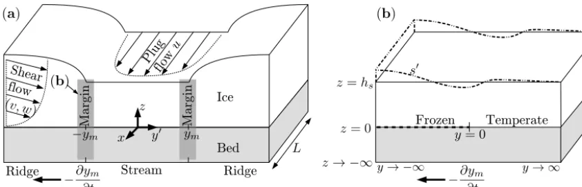
The model for ice stream margins we use here is derived in Haseloff et al. (2015). Let(x, y0, z)be a fixed coordinate sys-tem. The model assumes a well-developed ice stream, whose principal flow direction is aligned with the positivex direc-tion, as shown in Fig. 1a. The y0 axis is transverse to the ice stream, and thezaxis is vertical. The ice stream is bor-dered by slowly moving ice ridges. The model for the ice stream margin is located at the transition from ice stream flow regime to ice ridge flow regime, providing the coupling between the two.
In contrast to typical “shallow” ice stream and ice sheet models (Fowler and Larson, 1978; Morland and John-son, 1980; Hutter, 1983; Muszynski and Birchfield, 1987; MacAyeal, 1989; Blatter, 1995; Pattyn, 2003), which assume a small aspect ratio between vertical and lateral extent, the width of the margin region captured by the boundary layer model is on the order of the ice stream thickness. Conse-quently, the far fields of the ice ridge and ice stream are at-tained aty± ∞(see Fig. 1b).
The asymptotic analysis in Haseloff et al. (2015) shows that the boundary layer evolves rapidly in comparison to the ice stream and ice ridge, and is consequently quasi-static, with the only time-dependence arising from the moving tran-sition between a frozen and a temperate bed at ±ym(x, t ). Morever, Haseloff et al. (2015) show that the surface of the ice stream margin is flat at leading order and located at
z=hs, wherehsis the ice thickness of the ice stream. The ice–bed interface is assumed to be flat and located at
z=0. Note, however, that this assumption does not preclude the application of our results to ice streams with a weak topo-graphic control, as found in many regions of the Siple Coast: this assumption merely requires the elevation gradient of the bed to be sufficiently small that the bed elevation does not vary significantly over lateral distance of a few ice thick-nesses.
We define the margin locationy0= −ym(x, t )as the point where the bed goes from being at the melting point to be-low the melting point. To facilitate our analysis, we imme-diately change to a moving coordinate frame in which the transition from a temperate to a frozen bed is stationary at
y=0; see Fig. 1b. In other words, ify0is the stationary co-ordinate withy0=0 in the ice stream center and the margin aty0= −ym(x, t ), then the lateral coordinateyof the margin model is linked toy0through
y=y0+ym(x, t ), (1)
withy=0 at the transition from frozen to temperate bed (see Fig. 1b).yincreases towards the ice stream, with negativey
corresponding to the ice ridge side of the domain. The bound-ary layer is moving at velocity−∂ym/∂twith respect to the fixedy0axis.
The boundary layer is effectively two-dimensional: the ice stream is much longer than a single ice thickness, and
there-fore along-flow variations in mechanical and thermal condi-tions in thexdirection are much smaller than corresponding variations in the transverse and vertical directions. In other words, thexcoordinate is passive and(y, z)are the indepen-dent variables in the model.
We assume that the thermal state of the ice–bed interface controls the basal boundary conditions for the ice. This re-quires us to model the thermal response not only of the ice but also of the bed. We therefore specifically include the bed in the domain and apply a geothermal heat flux atz→ −∞. At the lateral domain boundaries aty± ∞, far-field bound-ary conditions are determined by coupling with stream and ridge.
Force balance can be separated into a downstream com-ponent, withudenoting the velocity component in thex di-rection, and a transverse component in the(y, z)plane, with
(v, w)denoting the corresponding transverse velocity plane. In the downstream direction, the velocityuis determined by
∂ ∂y η∂u ∂y + ∂ ∂z η∂u ∂z
=0, (2)
withηas the viscosity. The transverse velocity field is de-termined by the two-dimensional Stokes and mass balance equations:
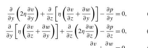
∂ ∂y
2η∂v
∂y + ∂ ∂z η ∂v ∂z+ ∂w ∂y −∂p
∂y =0, (3a)
∂ ∂y η ∂v ∂z+ ∂w ∂y + ∂ ∂z
2η∂w ∂z
−∂p
∂z =0, (3b)
∂v ∂y+
∂w
∂z =0. (3c)
The viscosity η depends on all three velocity components through Glen’s law (Paterson, 1994):
η=A
−1/n
21/n " ∂u ∂y 2 + ∂u ∂z 2 + ∂v ∂z+ ∂w ∂y 2 +2 ∂v ∂y 2 +2 ∂w ∂z
2#12−nn
, (4)
withAbeing the usual viscosity parameter andnthe rheol-ogy exponent. For simplicity, we neglect the effect of tem-perature on viscosity here.
The ice stream imposes a lateral shear stressτs as a far-field boundary condition. Additionally, the plug flow in the ice stream requires a vertically uniform across-stream veloc-ity in this far field, so
η∂u ∂y →τs,
∂v
∂z →0, w→0 fory→ ∞. (5)
direc-Figure 1.Panel(a)shows large-scale model geometry: we assume an ice stream flowing in positivexdirection. At its sides, the ice stream is bordered by slowly moving ice ridges. Panel(b)shows boundary layer geometry, which moves at the ratevm=∂ym/∂tthrough the ice stream/ridge geometry shown in panel(a).
tion:
u→0
v→ (n+2)
(n+1) qr
hs
"
1−
1− z
hs
n+1#
w→0
fory→ −∞, (6)
withqrbeing the ice flux from the ice ridge towards the ice stream andhsthe ice thickness of the ice stream; the form of
v corresponds to a “shallow-ice”-type shearing flow with a temperature-independent rate factorA.
We assume that basal melting has a negligible effect on ice velocities, so
w=0 atz=0. (7)
On the temperate (stream-ward) side of the ice–bed interface, we assume that the basal shear stress is negligible compared with the shear stresses in the ice, leading to a free-slip bound-ary condition:
η∂u ∂z =η
∂v
∂z =0 fory >0, z=0. (8)
In posing this boundary condition for an ice stream that is actively widening, we are assuming that an infinitesimal amount of melting of the bed suffices to allow for slip: once the thermal barrier at the bed is breached, we only need a very thin ice-free layer in order for slip to occur. This is con-sistent at least with the idea of a plastic bed, where slip can happen on a plane, or with a hard bed.
To the extent that additional degrees of freedom (other than temperature) are involved in sliding, the main concern would presumably be water pressure at the bed or within the till, rather than the thickness of the unfrozen till layer. Our assumption of a free slip once the melting point is reached is best justified (see Haseloff et al., 2015) if we suppose that the unfrozen bed is hydraulically well connected, so that the water pressure in the parts of the bed that have just become
unfrozen quickly equilibrates with water pressure elsewhere under the ice stream (and hence basal friction is comparable to the rest of the active ice stream). Shear stresses experi-enced by the margins of the ice stream are large compared with basal drag throughout the ice stream (Haseloff et al., 2015), and this implies that basal friction is small at leading order everywhere where the melting point is reached. There are undoubtedly other, more elaborate models for basal shear stress of the unfrozen bed; ours is the simplest possible case to analyze.
Where the bed is frozen, we consider two different possi-bilities. The first assumes that no slip is possible, so that the basal boundary condition fory <0 is
u=v=0 fory <0, z=0. (9a)
We also investigate the possibility of slip at significant basal friction on the frozen bed. For simplicity we use the simplest possible version of this problem and assume that the frozen ice–bed contact fails at a fixed yield stressτc(Schoof, 2004, 2010):
either η∂u ∂z=τc
u √
u2+v2, η
∂v ∂z=τc
v √
u2+v2, p
u2+v2>0 or
s
η∂u ∂z
2 +
η∂v
∂z 2
≤τc, p
u2+v2=0
for y <0, z=0. (9b)
The no-slip case (Eq. 9a) can be obtained formally by putting
τc= ∞in Eq. (9b).
The upper surface is traction-free and flat at leading or-der. In practice, this implies vanishing shear stress and nor-mal velocity, with vanishing nornor-mal stress accounted for by a first-order correction to the constant leading-order surface elevation. If the actual upper surface is located aths+s0with
s0hs, then
η∂u ∂z=η
∂v
∂z=w=0, 2η ∂w
∂z −p+ρgs
0
Thus, even though our model geometry is a parallel-sided strip, it takes into account the first-order surface slope to-wards the ice ridge.
Note that we have formulated the flow problem in such a way that it can be solved without reference to the temperature field. Physically, however, we require that the temperature
T is below the melting pointTm for y <0,z=0 and that the temperature is at the melting point for y≥0,z=0. To ensure that these conditions are met, we have to solve the heat equation in the ice (0< z < hs) and in the bed (z <0). The englacial heat production in the ice is balanced by conductive and advective heat transport, as well as a pseudo-advective term which is the result of the ice stream margin migrating at the rate
vm:=
∂ym
∂t (11)
into the ice ridge. (Physically, this term represents the effect of having to warm the initially cold ice in the ice ridge as the margin migrates into the ridge.) In the bed, no heat is dissipated and the bed is assumed to be static, so that we have a balance between the same pseudo-advective term and diffusion of heat:
ρcp
vm ∂T ∂y +v
∂T ∂y +w
∂T ∂z
−k
∂2T
∂y2+ ∂2T
∂z2
=a for 0< z < hs, (12a) ρbedcp,bedvm
∂T ∂y −kbed
∂2T
∂y2 + ∂2T
∂z2
=0 forz <0, (12b) where we used the margin migration velocityvmas defined by Eq. (11).ρ andρbed are the densities of ice and bed, re-spectively; cp andcp,bed are specific heat capacities; andk andkbed are thermal conductivities (see Table 1). The heat production termaprovides the thermomechanical coupling:
a=A
−1/n
21/n ∂u ∂y 2 + ∂u ∂z 2 + ∂v ∂z+ ∂w ∂y 2 +2 ∂v ∂y 2 +2 ∂w ∂z
2!12+nn
. (13)
Advection from the ice ridge prescribes a far-field tem-perature profile Tr(z), while there are no significant lateral temperature gradients towards the ice stream far field:
T =Tr(z) fory→ −∞,
∂T
∂y →0 fory→ ∞. (14)
To be consistent with a conduction-dominated temperature field, we assume for the far-field ridge temperature
Tr=
Ts+ qgeo
k (hs−z) ifz≥0 Ts+
qgeo
k
hs− k kbed
z
ifz <0.
(15)
We will show in Sect. 4 that the migration velocity is sensi-tive only to the far-field temperature at the bed, so the spe-cific form ofTris immaterial. Here we have assumed a linear profile for simplicity.
At the surface at z=hs, we assume a constant surface temperatureTs, and towardsz→ −∞we assume a constant geothermal heat fluxqgeo:
T =Ts atz=hs,−kbed
∂T
∂z →qgeo asz→ −∞. (16)
Finally, at the bed, we impose the following boundary condi-tions and inequality constraints:
T < Tm and
−k∂T ∂z +
+kbed
∂T ∂z − =
(0 ifτ
c= ∞ τc
p
u2+v2 ifτ
c<∞
fory <0, z=0, (17a)
T =Tm and
−k∂T ∂z +
+kbed
∂T ∂z − < (
0 ifτc= ∞ ∞ ifτc<∞
fory >0, z=0. (17b)
The two cases ofτccorrespond to whether subtemperate slip is or is not possible (τcbeing finite or infinite, respectively).
The equalities in Eq. (17) arise from the construction of our model: we have chosen the locationy=0 to separate a region with a temperate bed (y >0) from one where the bed temperature must be below the melting point but where it is not otherwise prescribed. In the latter case, a flux condition is necessary to ensure conservation of energy at the bed. Conse-quently, the temperature inequality in Eq. (17a) is an intrinsic part of how we have defined our domain, with the transition from a subtemperate to temperate bed occurring aty=0 in our traveling coordinate system.
The flux constraint in Eq. (17b) by contrast is really a con-straint on freezing rates on the temperate side of the thermal transition at the bed, and in imposing it we are assuming that the margin is migrating into the ice ridge at a ratevm>0. A local analysis of the temperature field neary=0 (see Ap-pendix A for a summary and Sect. S2 in the Supplement and Schoof, 2012, for details) demonstrates that, if the temper-ature constraint in Eq. (17a)1 is satisfied, then the net heat flux out of the bed for smally >0 either approaches+∞
Table 1.Parameter values used in the sample calculations presented here. Ice stream thicknesshs, lateral inflow of ice from the ridgeqr, and marginal lateral shear stressτs are highlighted as they repre-sent coupling with ice ridge and ice stream dynamics. hs and τs correspond to the values observed at the upper margin of Whillans ice stream (Harrison et al., 1998), which migrates at a rate of 7 to 30 m yr−1(Hamilton et al., 1998; Harrison et al., 1998; Echelmeyer and Harrison, 1999). Theqrestimate is based on an inflow velocity of 10 m yr−1.
Description Symbol Value Units Viscosity parameter A 1.6×10⁻¹⁵ kPa−3s−1
Rheological exponent n 3
Specific heat capacity cp,cp,bed 2 kJ kg−1K−1
Acceleration due to gravity g 9.81 m s−2 Thermal conductivity k,kbed 2.3 W m−1K−1
Geothermal heat flux qgeo 6×10⁻² W m−2
Density of ice ρ 920 kg m−3
Density of bed ρbed 920 kg m−3
Surface temperature Ts −25 ◦C
Melting point Tm 0 ◦C
Basal yield stress of ice ridge τc kPa
Ice stream thickness hs 900 m
Marginal inflow of ice qr 104 m2yr−1 Marginal lateral shear stress τs 200 kPa
from a finite value of τc to free slip implies a discontinuity in basal heat production and consequently requires a finite but non-zero basal freezing rate near the origin. In order to maintain the bed at the melting point, that finite freezing rate has to be compensated for by subglacial drainage (that is, a finite supply of latent heat into the very tip of the temperate bed region). We anticipate that future versions of this model will consider smooth transitions from subtemperate to tem-perate sliding, for instance by allowing the yield stress to ap-proach zero continuously as a function ofT. This, however, is computationally extremely onerous, and we persist with our simpler version of the basal physics here.
The inequality constraints serve the role of determining a unique migration ratevm. If we were to dispense with them, we could solve Eqs. (12a)–(16) with an arbitrary choice of
vm. However, for fixed model parameters, an arbitrary choice of vm will see one of the inequality constraints in Eq. (17) violated, and their role is therefore to specify the migration rate (see Sect. S1, and Schoof, 2012). That migration rate is then a function of geometrical and forcing parameters such as
hs,τs,qr, andqgeo.τs andqr in particular represent the far-field forcing due to coupling with ice stream and ice ridge. For instance, from the perspective of the ice stream,τsis the lateral shear stress it imposes on the boundary, while from the perspective of the ice ridge,qris the rate at which it supplies mass to the ice stream through the margin.
3 Solution of the model
We solve the coupled mechanical and thermal system Eqs. (2)–(17) with the finite-element solver Elmer/Ice (Gagliardini et al., 2013). The computational domain is a rel-atively large elongated rectangle which represents the mar-gin cross section in the(y, z)plane. It consists of an ice and a sediment subdomain. We apply the boundary conditions Eqs. (5)–(6) and Eqs. (14)–(16) at the relevant sides of the domain, rather than at±∞.
The solutions to the problem are uniquely determined by the lateral shear stressτs, the ice thicknesshs, marginal in-flow of ice from the ridgeqr, the geothermal heat fluxqgeo, and the surface temperatureTs, in addition to material prop-erties such as thermal conductivity, heat capacity, density, rheological parameters for the ice, and the basal yield stress
τc. We will treat the majority of these material properties as fixed (see Table 1) but consider carefully the effect of chang-ing the basal yield stress.
3.1 Ice flow and heat production
We begin with solutions to the ice flow problem (Eqs. 2– 10). In our model, we are treating viscosity and basal yield stress as independent from temperature. At present, this is necessary to allow the computation of more than a handful of solutions in a reasonable amount of time, mostly due to the difficulty involved in computing the migration rate from the inequality constraints (Eq. 17). The latter requires very fine grids and a costly iterative scheme (Haseloff et al., 2015). We anticipate that future versions of the model will consider two-way coupling between the mechanical and thermal processes, but in our simplified version we are able to compute solutions to the mechanical problem in isolation: givenhs,τs,qr,τcand the rheological propertiesAandn, we are able to compute velocity and pressure in the ice.
The downstream velocityuis vertically uniform in the ice stream far field and increases with a prescribed lateral gra-dient of 2Aτsn; see Eq. (5). Figure 2a1–c1show contours of
ufor differentτcplotted in the(y, z)plane, computed using the parameters in Table 1. Panels a2–c2show the correspond-ing across-flow field(v, w), whose magnitude is significantly smaller than the downstream velocity. Hence gradients of the downstream velocity u dominate the heat production rate, while the velocity(v, w)in the transverse plane accounts for the advection.
In the case of no slip on the cold side of the margin (y <0), stress is concentrated around the transition from no slip to free slip at the origin. This translates to very high dissipation rates (a) as shown in Fig. 2a3. It can be shown that there is in fact a singularity in shear stress, and consequently the heat production rate goes asa∼1/rat the origin in this case (Sect. S3; Rice, 1967).
Figure 2.Influence of the subtemperate yield stressτcon the mechanical fields in the ice stream margin.τsis the lateral shear stress in the margin. Rows of panels are labeled (a–d), with suffixes 1–3 indicating columns. Panels (a1–c1): contours of downstream velocity component
u at contour intervals of 40 m yr−1; bold line indicatesu=40 m yr−1. Panels (a2–c2): transverse velocity field(v, w)shown as arrows; shading indicates magnitude of the transverse velocity. Panels (a3–c3): contours of heat productionaat contour intervals 2.6×10⁻⁴W m−3,
a=2.56×10⁻³W m−3 shown as a bold line. Panels (d1–d3) show the velocities and heat dissipation at the bed. Note that no heat is dissipated at the bed where the velocities are zero. Calculations were done with the values listed in Table 1 andτcas indicated.
y <0 forms where the yield stressτc is attained and slid-ing occurs. Panels d1and d2show the velocitiesuandvat the bed (z=0). Allowing slip for y <0 leads to two ma-jor changes in the heat production. First, the englacial heat production is reduced and the singularity aty=0 is at least partially alleviated (see Fig. 2b3–c3; the local analysis with
n=1 presented in Sect. S2 indicates thata may still have a logarithmic singularity). Secondly, heat dissipation is intro-duced along the ice–bed interface (see Fig. 2d3). We will dis-cuss below how this shift in the location of heat production affects the temperature field in the ice.
Figure 2a2–c2show the transition of the transverse veloc-ity componentv from a shearing flow to a plug flow. At the boundaries of the domain the vertical velocity componentw
is zero. However, near the origin, we can observe a down-wards motion of ice todown-wards the bed, offsetting the accelerat-ing transverse flow. As foru, allowing for subtemperate slip in a small region aty <0 leads to a more gradual increase in velocities around the origin (see Fig. 2d1and d2).
3.2 Temperature field
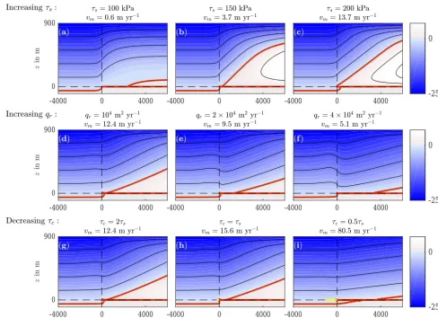
Figure 3.The effect of shear heating (represented byτs), advection (represented byqr), and subtemperate basal sliding (represented byτc) on the temperature field in an ice stream margin; same plotting scheme as in Fig. 2. Solid black lines show contours in 5◦C intervals with the contour ofT= 0◦C in red. Thin dashed lines indicate the ice–bed interface and the location of the cold–temperate transition at the ice–bed interface. Red shading indicates the formation of temperate ice. Note thatT should be interpreted as a proxy for moisture content when
T >0. In this case we can identifyφ=ρcpT /(ρwL), withφbeing the volumetric moisture content of the ice,ρwthe density of water, and
Llatent heat per unit mass. Panels(a–c)haveqr=0,τc= ∞(i.e., no subtemperate slip), and values ofτsas indicated above the panel. Panels(d–f)haveτs=200 kPa andτc= ∞. Panels(g–i)haveτs=200 kPa andqr=104m2yr−1. The yellow lines in panels(g–i)mark the extent of the subtemperate slip region. All other values as listed in Table 1.
In Fig. 3 we show temperature fields calculated with migration velocities that satisfy the inequality constraints (Eqs. 17a–17b). Each panel shows solutions obtained with a different combination of lateral shear stressτs, lateral inflow of cold iceqr, and basal yield stressτc. Increasingτs while holding all the other parameters constant (top row) leads to more heating of the ice around the slip transition point and inside the ice stream. Consequently, the migration velocity increases. This gives the bed and the ice to the left of the tran-sition point less time to heat up, and temperatures decrease there. The opposite effect can be observed for an increase of the lateral inflow of ice (second row), which reduces the mi-gration velocity and leads to a warmer bed. However, due to greater advection velocities, temperatures in the ice are lower (Fig. 3d–f).
Introducing subtemperate slip (decreasingτc) leads to ad-ditional heat dissipation along the ice–bed interface on the ridge side (y <0). This heat can thaw the frozen bed, thereby increasing the migration velocity. However, as in the case of increasingτs this gives the ice less time to heat up. Conse-quently, temperatures in the ice decrease asτcdoes.
Note that all the temperature fields shown in Fig. 3 have
2012; Schoof and Hewitt, 2016; Hewitt and Schoof, 2017): whereT >0, the productρcpT (which is generally the spe-cific heat content per unit volume of ice) must instead be interpreted as the latent heat content per unit volume of the ice. That is,ρcpT should be interpreted asρwLφ, whereρw is the density of water, L is latent heat per unit mass, and
φis the volumetric moisture content of the ice. This allows us to identifyφ=ρcpT /(ρwL), soT is nothing more than a proxy for moisture content whenT >0.
By solving the heat equation whereT >0, we make two main assumptions. First, qualitatively, we assume that mois-ture flows down gradients of moismois-ture, which is the assump-tion common to enthalpy gradient models and permits the same diffusive model to be applied regardless of whether the melting point has been reached or not. The second, quantita-tive assumption we make is that the corresponding diffusiv-ity remains the same for cold and temperate regions. This is consistent with prior work but also an obvious area for fu-ture model improvement. We will return to a discussion of the limitations imposed by this assumption in Sect. 5.
Importantly, the region of temperate ice in the bottom two rows of Fig. 3 does not form directly above the transition from subtemperate slip to free slip at the origin but is shifted significantly (by up to several ice thicknesses) towards the ice stream. This is the result of lateral advection of ice and of subtemperate sliding, which generates additional heat and requires less localized englacial heating (compare the local form of the temperature field in Appendix A and Sect. S2 with Appendix A of Schoof, 2012). This shift of the tem-perate region away from the slip transition suggests that the thermal physics around the transition from frozen to unfrozen bed may be relatively unaffected by the choice of temperate ice model (e.g., Aschwanden et al., 2012; Schoof and Hewitt, 2016; Hewitt and Schoof, 2017).
4 Migration velocity as a function of forcing parameters
We now turn to a systematic investigation of the dependence of the migration velocity on the ice ridge and ice stream pa-rameters. As we have pointed out, the solution to the veloc-ity and temperature problem is determined uniquely once we know the applied lateral shear stressτs, the inflow rate of cold ice qr, and the geothermal heat flux qgeo (or equivalently, the far-field bed temperature on the ridge side of the mar-ginTb), as well as ice thicknesshs, basal yield strengthτc, and the remaining material properties of ice and bed. Impor-tantly, that solution includes the margin migration rate vm, which is therefore a function of these physical parameters and material properties: defining the far-field basal tempera-ture through
Tb=Ts+
qgeohs
k ,
we can write
vm= ˆf (hs, qr, τc, τs, Tb;
A, cp, cp,bed, g, k, kbed, n, ρ, ρbed, Tm, Ts). (18) We emphasize ice thicknesshs, inflow rateqr, lateral shear stressτs, and far-field bed temperature under the ridgeTbin particular as these are parameters that reflect the coupling of the margin to dynamics of ice ridge and ice stream. Conceiv-ably, one might want to run a simulation that relies on sim-plified models of ridge and stream without having to resolve the margin region itself. The goal of a systematic solution of our margin model in that case is precisely to compute the mi-gration ratevmas a function of parameters that are controlled by the ridge and the stream: doing so allows the margin to be treated as a free boundary in a larger-scale model. We also emphasize the role of basal yield stressτc as we are inter-ested in how allowing for varying degrees of subtemperate sliding changes the relationship between margin migration rate and the forcing the margin experiences from ridge and stream.
It is clear that vm in Eq. (18) depends on a large num-ber of physical parameters, and the computational effort re-quired to find the function appears to be intractable. How-ever, we can reduce the parameter space to a minimum by non-dimensionalizing the model: doing so demonstrates that many combinations of parameter values actually correspond to scaled versions of the same calculation, which we then have to do only once. This is done in Sect. 4.1. An addi-tional advantage is that non-dimensionalization allows us to identify systematically which processes dominate the tem-perature field and migration rate (see Sect. 4.2). This leads to further simplification that allows us to give semi-analytical versions of Eq. (18) in a number of parameter regimes, which we study subsequently in Sect. 4.3–4.4.
4.1 Non-dimensionalization
The goal of this section is to express the model in the most succinct form possible. To do so we introduce
[z] =hs, [s0] =
n+2
n+1
qr
Aτn
sh2s
τs
ρg, [u] =Ahsτ n
s,
[v] =n+2 n+1
qr
hs
,[T] =Tm−Ts (19)
and put (y, z)= [z](Y, Z), u= [u]U, (v, w)= [v](V , W ),
s0= [s0]S0,p=ρg[s0]P, and T = [T]T +Tm. This allows us to absorb quantities such as the ice thickness, inflow rate, and dimensionless lateral shear stress in the ice stream mar-gin into five dimensionless parameters:
α= Aτ n+1 s h2s
k(Tm−Tb)
,Pe=(n+2) (n+1)
ρcpqr
k , ν= Tb−Ts
Tm−Ts
,
τ=τc τs
, ε=n+2 n+1
qr
Aτn
sh2s
Note that our parameterαis defined slightly differently from its counterpart in Schoof (2012) and Haseloff et al. (2015): if we replaceTmbyTs in the denominator of Eq. (20)1, we obtain the version ofαused in the latter two papers. We can interpret the parameters above as a dimensionless shear heat-ing rateα, a Péclet number (or measure of advection versus conduction)Pe, a dimensionless measure of the far-field bed temperatureν(νis between 0 and 1 for a ridge bed temper-atureTbbelow the melting pointTm, as we assume here), a dimensionless basal yield stressτ, and a ratio of transverse to downstream velocitiesε. Using the values in Table 1, we getPe=314,α=592,ν=0.9, andε=0.04.
Note that a large Péclet number is what we would expect in a spatially confined region like an ice stream margin: con-duction of heat is relatively ineffective, and advection mostly dominates. Large αreflects the strength of heat production, which must balance the fast rates of advection of cold ice implied by largePe. Note thatεremains small as long as the across-margin flow is significantly smaller than the down-stream flow, which we assume to be the case. Terms ofO(ε)
are retained only in order to regularize the viscosity in the ice ridge, where gradients inuvanish. In the numerical solu-tions presented in this study, we useε=0.01, and we have confirmed that smaller values of ε do not change our re-sults.O(1)values ofεwould imply that there is significant englacial heat production in the ridge; see Haseloff (2015) and Haseloff et al. (2015). This heat production should pre-vent the ice ridge bed from remaining frozen, contradicting our basic assumption that the shear margin is co-located with a thermal transition at the bed.τ is poorly constrained, and we will consider different parameter regimes ofτbelow. Ad-ditionally, we have the following ratios of material properties
γ =ρbedcp,bed ρcp
, κ=kbed
k . (21)
With the definitions above, the velocity in the downstream direction is determined by the scaled version of Eq. (2),
∂ ∂Y µ∂U ∂Y + ∂ ∂Z µ∂U ∂Z
=0, (22)
and the across-stream flow is described by Eq. (3):
∂ ∂Y
2µ∂V
∂Y + ∂ ∂Z µ ∂V ∂Z+ ∂W ∂Y −∂P
∂Y =0, (23a) ∂ ∂Y µ ∂V ∂Z+ ∂W ∂Y + ∂ ∂Z
2µ∂W ∂Z
−∂P
∂Z =0, (23b) ∂V
∂Y + ∂W
∂Z =0. (23c) µis the non-dimensional viscosity:
µ= 1
21/n " ∂U ∂Y 2 + ∂U ∂Z 2
+ε2 ∂V ∂Z + ∂W ∂Y 2 +2 ∂V ∂Y 2 +2 ∂W ∂Z
2!#12−nn
. (24)
The boundary conditions in the ice stream far field (Eq. 5) are now
µ∂U ∂Y →1,
∂V
∂Z →0, W→0 forY → ∞. (25)
Towards the ice ridge, we obtain from Eq. (6)
U→0, V →1−(1−Z)n+1, W →0 forY → −∞. (26) At the ice surface, we have from the boundary conditions (Eq. 10)
µ∂U ∂Z =µ
∂V
∂Z =W=0,2µ ∂W
∂Z −P+S 0
=0 atZ=1. (27) As before, basal melting has a negligible effect on ice veloc-ities, and Eq. (7) becomes
W=0 atZ=0. (28)
On the temperate side of the bed, we have free slip from Eq. (8):
µ∂U ∂Z =µ
∂V
∂Z =0 atZ=0, Y >0. (29)
On the frozen side of the bed, we can either have no slip (Eq. 9a),
U=V =0 atZ=0, Y <0, (30a)
or we allow subtemperate slip, requiring from Eq. (9b)
eitherµ∂U ∂Z =τ
U √
U2+ε2V2, µ
∂V ∂Z =τ
V √
U2+ε2V2, p
U2+ε2V2>0 or s µ∂U ∂Z 2 +ε2
µ∂V
∂Z 2
≤τ, pU2+ε2V2=0
forY <0, Z=0. (30b)
Note that the ice flow problem depends only onn,ε, andτ. For later convenience, we write the thermal problem in terms of a reduced temperature2through T =(1−ν)2− (1−ν)−νZ:2is the deviation from the linear temperature field that would result from geothermal heat flux and conduc-tion alone, given the imposed surface boundary value. Writ-ing the heat equation (Eq. 12a–12b) in terms of2yields
Vm
∂2 ∂Y +Pe
V∂2
∂Y +W ∂2 ∂Z +
ν
1−νW
− ∂22
∂Y2+
∂22 ∂Z2
Vmγ
∂2 ∂Y −κ
∂22
∂Y2+
∂22 ∂Z2
=0 forZ <0, (31b) with the heat production term
A= 1
21/n " ∂U ∂Y 2 + ∂U ∂Z 2
+ε2 ∂V ∂Z+ ∂W ∂Y 2 +2 ∂V ∂Y 2 +2 ∂W ∂Z
2!#12+nn
, (32)
where we have retained the smallO(ε2)term, analogous to that in Eq. (24). We have also introducedVm as the dimen-sionless speed with which the ice stream margin migrates outwards. It is related to the dimensional migration speed through
vm=
k ρcphs
Vm. (33)
The boundary conditions (Eqs. 14–16) are
2=0 atZ=1, (34a)
∂2
∂Z →0 forZ→ −∞, (34b)
2→0 forY→ −∞, (34c)
∂2
∂Y →0 forY→ ∞. (34d)
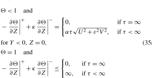
Finally, we have the inequality constraints determining the migration velocity, which are
2 <1 and
− ∂2 ∂Z +
+κ∂2 ∂Z − = (
0, ifτ = ∞
ατ √
U2+ε2V2, ifτ <∞
forY <0, Z=0, (35a)
2=1 and
− ∂2 ∂Z +
+κ∂2 ∂Z − ≤ (
0, ifτ = ∞ ∞, ifτ <∞
forY >0, Z=0. (35b)
We have now arrived at a model in which a (unique) di-mensionless margin migration velocityVmis defined by four dimensionless groups that depend on forcing from the ice stream and ridge (α,Pe,ν, andτ) and on the material con-stantsγ,κ, andn:
Vm=f (α,Pe, ν, τ, n, γ , κ). (36)
The remainder of this paper focuses on determining the form of the functionf. For comparison with previous work (Schoof, 2012; Haseloff et al., 2015), we additionally assume
γ =κ=1 andn=3, so thatVmcan only depend onPe,α,
ν, andτ. We start by treatingαandPeasO(1)parameters in
the next section to build intuition for the dependence ofVm onPe,α,ν, andτ and then investigate the physically more realistic case in which bothPeandαare large in Sect. 4.3– 4.4.
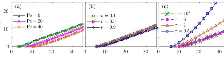
4.2 Migration velocities atO(1)values ofαandPe
In Fig. 4 we plotVmagainstαat fixed values of the other pa-rameters. We see a qualitatively similar picture to the cases described in Schoof (2012) and Haseloff et al. (2015), which assumed a constant viscosity (n=1): outward migration of the margin requires a minimum value of α. Once that is reached, the migration speed increases withα(Fig. 4a). In-creasing advection (Pe>0) in the heat balance reduces the corresponding migration speedVm. This is because heat pro-duction is now balanced not only by migration into the cold ice of the ridge but also by the influx of cold ice into the boundary layer (represented by Pe). In addition, for every fixed Péclet number there is a minimum nonzero value of
αthat generates a positive migration rate, as already found by Haseloff et al. (2015).
Solutions of Vm for differentν between 0.1 and 0.9 are shown in Fig. 4b. Note that the migration velocity is not very sensitive to changes inν: for increasingν, there appears to be a smallα-independent shift ofVmto smaller values. Con-sequently, relative differences in the migration rate should become smaller for increasing values ofα. If there are ad-ditional dependencies ofVmonν, these are small enough to be invisible. This behavior is consistent with the analysis for largeαthat we present later in Sect. 4.3.
We have seen in the discussion of the mechanical fields in Sect. 3.1 that subtemperate slip (τ <∞) introduces dissipa-tion along the ice–bed interface. Decreasingτ leads to more subtemperate slip and therefore to more dissipation at the bed on the cold side of the margin. Consequently we expect the migration velocity to increase with decreasingτ. Figure 4c confirms this. However, relatively small values ofτ.1 are needed before there is a noticable effect on the migration ve-locity.
ad-Figure 4.Dependence of non-dimensional migration velocityVmon lateral advection (parameterized byPe,a), far-field bed temperature (parameterized byν,b), and basal shear stress on subtemperate side of the bed (parameterized byτ,c). Unless indicated otherwise, we used
Pe=10,ν=0.5, andτ= ∞.
dress the more complicated case of finiteτ, concluding with formulae forVmin the parameter regimes of large and mod-erate subtempmod-erate slip.
4.3 Large heat production without subtemperate slip
We initially restrict ourselves to the case of no subtemper-ate slip and consider the case of large α: our estimates in Sect. 4.1 indicate that this limit is likely to apply in practice. Combined with a large heat production rate, the same esti-mates lead us to expect a large Péclet number: ice is a rela-tively poor thermal conductor, and advection dominates con-duction at the scale of a single ice thickness. Mathematically, this corresponds to advection and heating terms in the heat equation dominating over diffusion in Eq. (31) over most of the domain. However, this is no longer true close to the tran-sition from no slip to free slip where there is a small region in which conduction also contributes to the local energy bal-ance. The physics in this region determine the migration rate: conduction is an essential part of how the margin migrates, as it controls how heat production causes the cold part of the bed to warm, and how much heat is extracted from the temperate part of the bed. The analysis below therefore focuses on this small region (known technically as a “conductive boundary layer”; see Fig. 5a).
In what follows we give a brief description of how we can derive a model that ties migration velocity to heat production and transport in the conductive boundary layer. The reader not concerned with the technical details will find the result of this analysis in Eq. (43).
The non-dimensional mechanical problem (Eqs. 22–30b) is parameter-free in the absence of subtemperate slip (theτ= ∞case above). However, to analyze the temperature field in the boundary layer, we need to know the behavior of flow velocity and heat production near the transition from no slip to slip. In Sect. S3, we show thatA,U, and(V , W )exhibit
power-law behavior near the origin: A∼A−ϑ1R−1
U∼
r
2n n+1A
2 n+1
ϑ +cosϑ A
1−n 1+n
ϑ R
1 n+1
(V , W )∼(Vϑ, Wϑ)Rβ
asR=pY2+Z2→0, (37)
withβ=0.5 forn=1 and β≈0.271 for n=3, and Aϑ, Vϑ, and Wϑ functions of the angle ϑ between the vector (Y, Z)and the Y axis and independent of any other model parameters. Here,R=
√
Y2+Z2 is distance from the ori-gin. Knowledge of Eq. (37) enables us to study the behavior of the temperature field close toR=0.
For large α, heating near the origin behaves as αA∼ αR−1. As described above, we are looking for a region in which this heating rate is partially balanced by conduc-tion. This happens at distances from the origin that scale as
Rα=α−1. To resolve this region, we set(Y, Z)=Rα(eY ,eZ),
A=Rα−1Ae, and (V , W )=Rαβ(V ,e W )e using Eqs. (37)1 and (37)3, and put 2e=2. If the boundary layer sets the migration rate, then the effect of the margin migrating into colder ice must also enter into the energy balance of the boundary layer at leading order. In order for this to happen, we need a large migration velocity withVm∼α, which we capture by rescaling the migration velocity as
e
Vm=α−1Vm. (38)
We can simultaneously consider conditions under which ad-vection due to motion of the ice also contributes to the cool-ing of the conductive boundary layer, in addition to migration into cold ice. It turns out that this requiresα−(1+β)Peto be ofO(1); i.e., the Péclet number must scale asPe∼α1+β. We therefore put
3=Pe1+β1 1
α (39)
Bed
Ice:
Free slip No slip
Conductive bl (b)
sub-temperate slip
Conductive bl
Bed
Advective bl
(a) Ice:
Free slip
No slip :
Advective bl
Figure 5.Boundary layer structure for asymptotic calculations with largeαandPe, without subtemperate slip(a)and with subtemperate slip(b). The background temperature profiles are enlargements of typical profiles in this asymptotic limit, with same color scale as in Fig. 3. In the outer advective boundary layer the temperature field close to the bed is advected from the ice ridge towards the inner conductive boundary layer. In the case of a no-slip–free-slip transition at the bed the conductive boundary layer consists of a small region around the slip transition(a). In the case of subtemperate slip, the conductive boundary layer is a region of small vertical extent which stretches along the length of the subtemperate slip region(b). Within the conductive boundary layer, heat dissipation is balanced by diffusion.
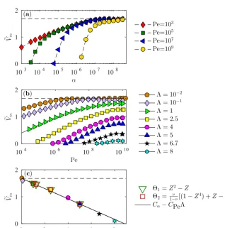
Figure 6. Asymptotic behavior of Vem=Vmα−1 for the case without subtemperate slip. In this case we expect a limiting behavior of
e
Vm=f (3)e forα1 and3=Pe1/(1+β)α−1; see Eq. (41). Panel(a):Vemagainstαfor different values of constantPe. Convergence to a constant value confirms the limiting behavior predicted by Eq. (41). Panel(b):VemagainstPefor different values of3. Note that holding3 constant asPechanges implies thatαchanges proportional toPe1/(1+β). Panel(c):Vemagainst3at constantPe=1010, corresponding to different values off (3)e . Filled markers show the same data as in panel(b). The open triangles and squares additionally show results for two
stream as we are assuming here, and we exclude the case of large3from consideration.
With these changes of variables and parameter definitions in place, Eq. (31) becomes (neglecting anO(α−1)term)
e Vm
∂e2 ∂eY
+3(1+β)
e V∂e2
∂Ye +We
∂e2 ∂Ze
−
∂2e2 ∂Ye2
+∂
2 e 2 ∂eZ2
=Ae for 0<Z,e (40a)
e Vm
∂e2 ∂eY
− ∂2
e 2 ∂Ye2
+∂
2 e 2 ∂eZ2
=0 foreZ <0, (40b) with boundary conditions given by the τ = ∞ case in Eq. (35) and each variable being replaced by its rescaled ver-sion (i.e., 2 being replaced by2e, Y by eY, and Z by Ze). This boundary layer model contains only Vem and3as pa-rameters; if (as we expect) there is a unique migration veloc-ityVemwhich solves this problem for given3, then we have
e
Vm=f (3)e .
However, we are still missing conditions on2eat large dis-tances from the origin, as we exit the conductive boundary layer and enter a region in which diffusion does not play the same leading-order role (see Fig. 5a). These far-field condi-tions dictate how cold the ice that is advected into the con-ductive boundary layer is and therefore control in part the strength of conductive heat loss. In order to conclude that
e
Vmdepends on the parameters in the original scaled model (Eq. 31) only through 3, we need to be certain that these far-field conditions one2also depend only on3. It turns out that these far-field conditions are determined by heat trans-port in a slender region near the bed. This region is marked with “advective boundary layer” in Fig. 5a; it extends above the origin and towards the cold ice ridge. In this region, shear heating is balanced predominantly by advection of cold ice into the margin and by the effect of having to warm up ice to-wards the melting point as the margin migrates into the ridge. It can be shown that, at leading order, the heat equation in this region again contains onlyVemand3as parameters and, consequently, that the far-field conditions to Eq. (40) depend only onVemand3as required. This is somewhat tedious, and we give details in Sect. S4. Ultimately, we are able to confirm theoretically that
e
Vm=f (3).e (41)
Our goal now is to check numerically that this relationship is obtained from direct solutions of Eqs. (22)–(35) whenαand
Peare made sufficiently large, and to find the approximate form of the functionfe. Note that we have gone from having a complicated function of 16 variables in Eq. (18) to being able to express the migration rate as a function of a single variable3(which in turn depends onαandPe). Approximat-ing a function of a sApproximat-ingle variable numerically, for instance in the form of a lookup table, is obviously much simpler than having to solve numerically for a large number of
indepen-dent variables, justifying the perhaps somewhat obscure pro-cedure that has led us to this point (and its equivalent forms for other parameter regimes to follow later).
The limiting behavior (Eq. 41) can also be written as
Vm=αfe
Pe1/(1+β) α
! .
Immediately, we see that for no advection (Pe=0) we expect a linear relationship between migration rateVm and heat-ing rateα, which the results in Schoof (2012) and Haseloff et al. (2015) already hinted at for largeα. In fact, a linear relationship does not require vanishing Pe: it suffices that
Pe1/(1+β)/α→0. We confirm this behavior numerically in Fig. 6a, whereVemis plotted againstαfor different fixed val-ues ofPe.Vemconverges to approximately 1.68 for each value ofPe, with the rate of convergence dependent onPe(Fig. 6a). A more general scenario is to considerα→ ∞andPe→ ∞in such a way that3is finite, in which case we cannot neglect the effect of advection. Figure 6b shows the conver-gence ofVemto its limiting formf (3)as we makePe(and henceα) large while holding3fixed. Note that holding3
fixed means thatαmust grow in lockstep withPe1/(1+β). The approach to the limit can be relatively slow, though the lim-iting value gives a good order-of-magnitude estimate of the actual migration rate even for smaller values ofPe.
Finally, by plotting the converged values of Vem at large
Peagainst 3, we can find the function f (3)e in Eq. (41). Figure 6c showsVem plotted against3 for a fixed value of
Pe=1010, which is large enough for the limiting value to have been approached closely in all the examples shown in Fig. 6b. We can fit a linear relationship to the computational data, of the form
e
f (3)=Cα−CPe3, (42)
with Cα≈1.68 and CPe≈0.19, preserving the limiting value off (e0)identified above. Written in terms of the origi-nal migration velocityVm=αf (3)e , this is the same as Vm=Cαα−CPePe
1
1+β (43)
forα1 andPe1. As previously noted (see also Schoof, 2012; Haseloff et al., 2015), a finite heating rateαis required in order to cause outward migration of the margin, and the formula above is only valid for argumentsαandPethat en-sureVm>0.
boundary layer is not sensitive to the details of the tempera-ture profile with which ice enters the margin from the ridge, except for the basal temperature of ice in the ridge: ice at higher elevations simply passes over the boundary layer and does not affect the energy balance that controls the migration rate at leading order. In technical terms, the far-field bound-ary conditions on2ecome from matching with the advective boundary layer alluded to above, which itself occupies only a small region near the bed and therefore has inflow boundary conditions dictated by the near-bed temperature prescribed in the limitY → −∞; see Sect. S4 for details.
We can confirm computationally from solutions to Eq. (31) thatVmis insensitive to the temperature profile im-posed on the left-hand boundary. Still using large values of
α andPe, we solve Eq. (31) with the purely diffusive tem-perature profile prescribed in Eq. (34c) replaced by several nonlinear ones that have the same temperature at the bed as Eq. (34c), but with a steeper temperature gradient near the bed. The corresponding migration rates are displayed as open (empty) markers in Fig. 6c, and we find close agreement between results obtained from different far-field temperature profiles.
4.4 Large heat production with subtemperate slip In the last section, we considered large dissipation rates and rapid advection of ice but not subtemperate slip. The migra-tion velocityVm is then determined by heat production and transport in a small conductive layer around the no-slip-to-slip transition. The extent of that boundary layer scales as
Rα=α−1. Here, we extend the analysis for largeαandPe
to account for subtemperate slip. When we allow for sub-temperate slip in our model, sliding occurs on a patch of bed of finite size Rc, and the size of that patch relative to the size of the diffusive boundary layer Rα becomes a key
consideration (see Fig. 5b). We need to distinguish two ba-sic cases,Rα∼RcandRc∼O(1). We treat the former case first. Our modus operandi also remains the same as in the previous section: by rescaling the dimensionless temperature model (Eq. 31) to capture the leading-order behavior in the conductive boundary layer that determines the migration ve-locity, we derive a simplified form for the migration rateVm as a function of the dimensionless parametersα,Pe,ν, andτ, and test that relationship by solving Eq. (31) directly in the appropriate parameter regime.
4.4.1 A small slip region:τ∼α1/(n+1)1
Consider a slip region that is similar in size to the conductive boundary layer of Sect. 4.3. To have such a small slip re-gion, the dimensionless yield stressτ must be large.τ scales as τ ∼ |∂U/∂Y|1/n, and with Eq. (37) we find that dimen-sionless stresses in the ice scale asR−1α /(n+1)=α1/(n+1)in
the conductive boundary layer of Sect. 4.3. These must now be comparable to the dimensionless yield stress of the bed;
hence
τ∼α1/(n+1).
As we reduceτ from an effectively infinite value (so there is no slip, as in Sect. 4.3) until it is comparable toα1/(n+1), the magnitudes of velocity components and heat production rate in the conductive boundary layer remain the same as in Sect. 4.3, but the dependence of velocity and heat pro-duction on position starts to change, so the analytical for-mulae (Eq. 37) no longer apply directly. (Technically, these formulae remain valid at distances r from the origin for whichRαr1.) Knowing that the magnitudes remain the same, however, we can use the same rescaling as in Sect. 4.3; put Rα=α−1; and set (Y, Z)=Rα(eY ,eZ), A= Rα−1Ae, U=R
1/(n+1)
α Ue, (V , W )=Rαβ(V ,e W )e , and 2e= 2.
The resulting mechanical problem is detailed in Sect. S5. We do not go into detail here: the point is that the velocity
(U ,e V ,e W )e and hence the heat production rate Aeare fully determined if the ratio of yield stressτ to typical stress level
α1/(n+1)in the conductive boundary layer is given. We write that ratio (effectively, a dimensionless slip parameter) here in the form
0=τ−(1+n)α. (44)
Note that Sect. 4.3 effectively treated the case of no slip,0=
0, and we seek to generalize this here. The corresponding problem for temperaturee2again takes the form of Eq. (40). In addition toAenow being dependent on the slip parameter 0, the boundary conditions at the bed also depend on0: we have from Eq. (35a)–(35b) that
−∂e2 ∂Ze +
+∂2e ∂Ze −
=0n+−11|Ue| oneZ=0,eY <0, (45a) e
2=1 oneZ=0,eY >0, (45b) with the inequality constraints on flux and temperature still taking the same form as in Eq. (35a)–(35b).
In other words, the conductive boundary layer problem now depends on an additional parameter through0: with the abrupt transition from no slip to free slip (Sect. 4.3), we had e
Vm=f (3)e ≈Cα−CP e3, while now we have e
Vm=eg(3, 0), (46)
withf (3)e =eg(3,0). To confirm that Eq. (46) holds, we fix 3and0to specific values and increaseα. This implies that
Pe=(α/3)1+βandτ =(α/ 0)1/(1+n)both increase in lock-step withα. Convergence ofVemto a value that depends only on3and0forα→ ∞then confirms Eq. (46).
Figure 7.Panel(a): asymptotic behavior forτ1 where we expect a limiting behavior ofVem=eg(3, 0)forα1; see Eq. (46).
Con-vergence to constant values confirms the limiting behavior. Note that αis plotted on a logarithmic scale. Panel (b): velocities against
0=τ−(n+1)αat constant values of3=Pe1/(1+β)α−1as indicated by color andα=107.25. Note that0→0 corresponds toτ→ ∞, the limit without subtemperate slip.
where we have restricted ourselves to only three values of
3 and focused on the effect of changing the slip parame-ter0. Figure 7a shows the expected convergence in the limit of largeα. As in Sect. 4.3, convergence often requires quite large values ofα. The limiting value ofVemis plotted against
0for the three different values of3used in Fig. 7b. As already observed in Sect. 4.2, decreasing the basal shear stress increases the migration velocity due to increased dissipation on the cold side of the bed. We observe the same here, in the sense that increasing0∝τ−(n+1)increases the migration velocity. We also reproduce the limiting behavior for 0→0 (τ→ ∞), in which case we expect to reproduce the migration rate predicted for the no-slip-to-free-slip tran-sition case of Sect. 4.3. In fact, Fig. 7b shows that relatively large values of 0≈10 are needed to see a significant de-parture of migration velocityVemfrom its limiting value for
0=0. Unfortunately, computational constraints make it im-possible for us to find a simple closed-form approximation foreganalogous to Eq. (42): we simply do not have enough data to construct such an approximation. However, we will present a solution to this issue in Sect. 4.4.3.
4.4.2 AnO(1)slip region:τ∼O(1)
We now turn to the case ofτ ∼1, in which the lateral shear stressτsexerted by the ice stream on the margin is compara-ble with the yield strengthτcof the frozen bed. In this limit, we expect the subtemperate slip length scale to be compara-ble with ice thickness, soRc∼O(1)(see also Fig. 2). The region in which there is significant dissipation along the bed is now much larger than in the previous section. As a re-sult, the region in which dissipation is balanced substantially by conduction now has a horizontal extent comparable with ice thickness, too. For largeα, however, we still have a con-ductive boundary layer whose vertical extent remains small: large temperature gradients are needed in order to account for the large amounts of dissipation, and such temperature
gradients have to correspond toO(1)temperature changes occurring over small vertical distances. In fact, that vertical distance still scales asRα=α−1. The primary difference is therefore that the boundary layer now has anO(1)extent in the horizontal, equal to the size of the slip region.
With an O(1) region of slip at the bed, there are no simplifications to the mechanical problem (Eqs. 22–30b): we are no longer confining our attention to a small region around the origin. The solution to the mechanical problem is fully specified if we knowτ, so(U, V , W )are functions of τ only. The horizontal velocity components (U, V ) are of O(1). If we are concerned with the conductive bound-ary layer near the bed, then we only need the vertical ve-locity component near the bed. SinceW=0 at the bed it-self, we find that W∼Z in the boundary layer. This al-lows us to rescale as (Y, Z)=(Y∗, RαZ∗), (U, V , W )= (U∗, V∗, RαW∗),A=A∗, and2=2∗. The leading-order version of the heat equation (Eq. 31) is thus (neglecting terms ofO(α−1))
Vm∗∂2
∗
∂Y∗ +
V∗∂2
∗
∂Y∗ +W ∗∂2∗
∂Z∗
−∂
22∗
∂Z∗2
=0, (47a)
Vm∗∂2
∗
∂Y∗−
∂22∗ ∂Z∗2
=0, (47b) where we defined
Vm∗=Vm α2, =
P e
α2 (48)
and retainedas anO(1)quantity: doing so withα1 is again to look at a distinguished limit, analogous to treating
3asO(1)in Sect. 4.3. The rescaled version of the heat flux constraint (Eq. 35a2) is
−∂2
∗
∂Z∗ +
+ ∂2
∗
∂Z∗ −
=τ|U∗|.
advection occurs from the ice ridge, which fixes the far-field temperature at 2∗=0 as Y∗→ −∞, so there is no additional parameter dependence through the far-field condi-tions. The thermal problem (Eq. 47) contains only the dimen-sionless parameters andτ (the latter both explicitly and through the velocity field). This indicates that the rescaled migration velocityVm∗only depends onandτ:
Vm∗=g∗(, τ ) (49)
for α1, Pe∼α2, and τ ∼1. Expressed in terms of the original migration velocityVm, we have
Vm=α2g∗ Pe
α2, τ
.
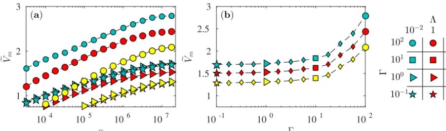
Once more we confirm that the formula (Eq. 49) holds by computingVm∗for different fixedandτwhile increasingα. In this case, we can observe convergence at moderately large values ofα≈102to 103(Fig. 8a). Again, smaller values of
τ lead to larger values ofVm∗, and increasingPe(and hence
) leads to decreasingVm∗(Fig. 8b). Note that the solutions shown are computationally expensive: the conductive bound-ary layer invariably requires local mesh refinement, and in the parameter regime considered here it extends over a larger part of the domain, with the size of the region that requires mesh refinement depending onτ. As a result, we are not able to compute solutions for very large values ofαat all values of τ. Therefore, computational constraints once more mean that we are unable to sample a large enough region of the two-dimensional parameter space to give a simple formula for the functiong∗.
However, for small values of τ 1, it is possible to solve the boundary layer problem analytically, as shown in Sect. S6. Effectively, this corresponds to finding the limiting behavior ofg∗asτ →0, for which we obtain withn=3 that
g∗(, τ )∼1 τ
64
315√π −
63√π
64 τ 2
, (50)
where the solution is valid only when the term in square brackets is positive: as before, a minimum value ofα (equiv-alent to a maximum value of∝α−2) is required to ensure outward migration of the margin. This limiting form is dis-played in Fig. 8b along with the computationally obtained migration velocities for nominally small values of τ =1,
τ =0.5, andτ=0.25 (note thatVm∼τ−1, soVmdoes not approach a finite value but diverges in a predictable fash-ion). Forτ=1 andτ =0.5, there is still a notable difference between the numerical solution and the analytical solution (Eq. 50), implying that these values ofτ do not yet satisfy
τ 1. However, for τ =0.25, the difference between the numerical solution and the analytical solution is negligibly small.
4.4.3 Moderate slip: 1τ α1/(1+n)
One of the difficulties we still face in making our results directly applicable to large-scale models is that we have a closed-form approximation for the migration rateVmfor only two parameter regimes. Both assume large dissipation rates
α1, which is realistic for abrupt ice stream margins. One applies to the case of no subtemperate slip (Eq. 43), while the other applies to extensive subtemperate slip (Eq. 50). The obstacle to dealing with more moderate amounts of subtem-perate slip is that the functionsegandg∗in Eqs. (46) and (49) are both functions of two independent variables and that they are computationally expensive to evaluate.
There is one regime in which we can do better and re-duceeg andg∗effectively to functions of a single variable: both functions have to be valid representations of the mi-gration velocityVmin the limit 1τ α1/(1+n), in which
0=τ−(1+n)α andτ are both large. In other words, in this parameter regime, we expect thategandg∗give the same an-swer:
Vm∼αeg(3, 0)∼α 2g∗
(, τ ).
If we denote the limiting forms ofegandg∗in the parameter limit under consideration with a subscript 0, then eliminating
andτ in favor of0,3, andαleads to
αeg0(3, 0)=g∗0
31+βαβ−1, α1/(1+n)0−1/(1+n)
.
By choosingPeandτ, we can vary3and0independently ofα. Hence, for any given0and3, we can now pickα=0
and are left with eg0(3, 0)=0
−1g∗ 0
31+β0β−1,1, (51)
where we only need to evaluate g0∗ at a fixed value of its first argument in order to compute Vm/ 0. Define g(χ )=
g0∗(χ1−β,1)for arbitraryχ. It then follows that we can use Eq. (51) andVm=αeg0(3, 0)to write
Vm=τ−(1+n)α2g
τ(1+n)Pe1/(1−β)α−2/(1−β)
. (52)
As promised, the migration rate once more reduces to a func-tiongof a single variable.
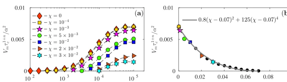
Finding an approximation togrequires significantly fewer function evaluations. Instead of varyingτ,Pe, andα, we only need to vary the argumentχ=τ(1+n)Pe1/(1−β)α−2/(1−β) of the functiong. As before, we first confirm that Eq. (52) in-deed holds by holding χ fixed and increasing α (Fig. 9a). Subsequently, we plot the limiting value of Vmτ1+nα−2 againstχin Fig. 9b. A simple polynomial fit
g(χ )≈hc2(χ−χ0)2+c4(χ−χ0)4 i
Figure 8.Panel(a): asymptotic behavior forτ∼1 where we expect a limiting behavior ofVm∗=Vmα−2=g∗(, τ )forα1; see Eq. (49). The limiting behavior is confirmed by convergence to constant values forα1. Panel(b): asymptotic behavior ofVm∗against=Peα−2
along constant values ofτat values ofαwhere convergence is observed. Dashed lines show the analytical solution (Eq. 50), which is valid forτ1.
Figure 9.Asymptotic behavior for largeαandPefor the case of intermediate slip (1τ.α1/(1+n)) where we expect a limiting behavior of
Vmτ(1+n)α−2=g(χ ); see Eq. (52). Panel(a):Vmτc1+n/α2againstαfor different values ofχ=τc(1+n)Pe1/(1−β)α−2/(1−β)withPefixed between 0 and 107andτ varying between 0.1 and 3.2. Convergence to constant values forα1 confirms Eq. (52). Panel(b): values of
Vmτc1+n/α2at differentχforα=105andτ=3.2.
5 Discussion and conclusions
In this study, we have investigated how different physical processes determine the widening of ice streams that are not topographically confined. We have considered the case in which the transition from fast to slow or no sliding that characterizes a typical ice stream margin is co-located with a thermal transition at the bed. In this scenario, the often in-tense dissipation of heat generated by the change in sliding behavior can cause the corresponding transition from a tem-perate to a cold bed to move, and the main objective of this study is to determine the corresponding rate of margin migra-tion into the cold region. This ice stream widening relies on a delicate balance between heat dissipation, heat transport by advection, and conduction to warm the initially cold bed out-side the ice stream. We have specifically excluded the case where heat loss dominates and the margin migrates into the ice stream from consideration here, although similar physics would allow inwards migration to be modeled (Schoof, 2012; Haseloff, 2015).
How the margin location is determined here differs from existing studies of heat transfer processes in Schoof (2004),