www.earth-surf-dynam.net/4/309/2016/ doi:10.5194/esurf-4-309-2016
© Author(s) 2016. CC Attribution 3.0 License.
A nondimensional framework for exploring the relief
structure of landscapes
Stuart W. D. Grieve1, Simon M. Mudd1, Martin D. Hurst2, and David T. Milodowski1
1School of GeoSciences, University of Edinburgh, Drummond Street, Edinburgh EH8 9XP, UK
2British Geological Survey, Keyworth, Nottingham NG12 5GG, UK
Correspondence to: Stuart W. D. Grieve ([email protected])
Received: 9 December 2015 – Published in Earth Surf. Dynam. Discuss.: 14 January 2016 Revised: 17 March 2016 – Accepted: 30 March 2016 – Published: 8 April 2016
Abstract. Considering the relationship between erosion rate and the relief structure of a landscape within a nondimensional framework facilitates the comparison of landscapes undergoing forcing at a range of scales, and allows broad-scale patterns of landscape evolution to be observed. We present software which automates the extraction and processing of relevant topographic parameters to rapidly generate nondimensional erosion rate and relief data for any landscape where high-resolution topographic data are available. Individual hillslopes are identified using a connected-components technique which allows spatial averaging to be performed over geomorphologically meaningful spatial units, without the need for manual identification of hillslopes.
The software is evaluated on four landscapes across the continental United States, three of which have been studied previously using this technique. We show that it is possible to identify whether landscapes are in to-pographic steady state. In locations such as Cascade Ridge, CA, a clear signal of an erosional gradient can be observed. In the southern Appalachians, nondimensional erosion rate and relief data are interpreted as evidence for a landscape decaying following uplift during the Miocene. An analysis of the sensitivity of this method to free parameters used in the data smoothing routines is presented which allows users to make an informed choice of parameters when interrogating new topographic data using this method. A method to constrain the critical gradient of the nonlinear sediment flux law is also presented which provides an independent constraint on this parameter for three of the four study landscapes.
1 Introduction
The Earth’s surface evolves dynamically in response to the interplay of climatic, tectonic and other factors operat-ing at timescales rangoperat-ing from minutes to millennia. High-resolution topographic data generated from terrestrial and airborne laser scanning, in combination with increased com-putational power, has facilitated a revolution in geomor-phology, allowing the quantitative interrogation of landscape form to provide insight into the forces shaping a landscape. Relationships have been found between topography and the tectonic (e.g., Wobus et al., 2006; Hilley and Arrowsmith, 2008; DiBiase et al., 2012; Hurst et al., 2013a), climatic (e.g., Gabet et al., 2004; Anders et al., 2008; Champagnac et al., 2012), and biotic (e.g., Roering et al., 2010; Milodowski et al., 2015a) forcing of a landscape in addition to links
be-tween topography and bedrock properties (e.g., Korup, 2008; Clarke and Burbank, 2010, 2011; Hurst et al., 2013b).
Our approach is rooted in a nondimensional framework that describes relationships between erosion rates and hills-lope topography in soil-mantled landscapes (Roering et al., 2007). This framework facilitates the direct comparison of landscapes of widely varying morphology and process. It has been shown to provide compelling insight into the identifi-cation of landscape transience (Hurst et al., 2012), complex tectonic signals from topography (Hurst et al., 2013a), and process controls on the density of channels (Sweeney et al., 2015). Extracting the nondimensional parameters from high-resolution topography can be difficult, subject to choices about how the metrics are calculated, and there has been no investigation into how different methods might influence re-sults, and therefore the interpretation of landscapes.
Here we present a framework and methodology for ex-tracting the required topographic parameters and processing the resulting data. Our software uses a clear methodology to allow researchers to generate these data for new landscapes and can replicate published relationships between nondimen-sional erosion rate and relief. Such relationships can be used to discriminate between landscapes in topographic steady state, where erosion rate is balanced by uplift rate, and those undergoing transience or topographic decay.
Additionally we present a method for generating spatially contiguous hilltop patches, required as a spatial averaging tool in many studies (e.g., Perron et al., 2009; Hurst et al., 2012, 2013a) to identify individual hillslopes for analysis. An analysis on the influence of spatial averaging and data smoothing on the interpretation of topographic data is under-taken and hillslope and basin average data are also used to estimate the critical gradient, a key parameter in the nonlin-ear sediment flux model.
2 Theoretical background
Numerous sediment flux laws (cf. Dietrich et al., 2003) have been developed and tested, particularly since the advent of cosmogenic radionuclide dating and high-resolution topo-graphic measurements. In addition to the conceptually sim-ple linear flux law (Culling, 1960; McKean et al., 1993; Tucker and Slingerland, 1997; Small et al., 1999; Booth et al., 2013), models of depth-dependent (Braun et al., 2001; Furbish and Fagherazzi, 2001; Heimsath et al., 2005; Roer-ing, 2008) and nonlinear sediment flux (Andrews and Buck-nam, 1987; Roering et al., 1999, 2001, 2007) have been em-ployed, alongside models which directly consider sediment particle motion (Foufoula-Georgiou et al., 2010; Tucker and Bradley, 2010; Furbish and Roering, 2013).
Models which consider particle motion are challenging to apply to real topography as they do not have an analytical so-lution and without high-resoso-lution soil depth information it is challenging to apply a soil-thickness-based sediment flux law to landscape-scale analysis (Grieve et al., 2016b). However, topographic predictions of the nonlinear flux law have been
successfully tested (Roering et al., 2007; Grieve et al., 2016b) suggesting that it, at a minimum, can constrain broad-scale sediment transport processes across landscapes. The nonlin-ear flux law is (Andrews and Bucknam, 1987; Roering et al., 1999, 2001, 2007)
¯ qs=
KS 1−(|S|/Sc)2
, (1)
where S is the topographic gradient in dimensions of
length/length (dimensions denoted in square brackets as [L]ength, [M]ass and [T]ime),Sc[dimensionless] is the
hill-slope critical gradient, K [L2T−1] is a sediment transport coefficient, andq¯s[L2T−1] is a volumetric sediment flux per
unit contour length. AsStends towardsSc, the sediment flux
asymptotically increases towards infinity, corresponding to an increase in landsliding on an increasingly planar hillslope. Roering et al. (2007) modeled the relief structure of theo-retical one-dimensional hillslopes which evolve under Eq. (1) and found that relief, the difference in elevation between a hilltop and the point on the channel it is coupled to, is con-trolled by the erosion rate, hillslope length, and the sedi-ment transport coefficient. Equation (1) has been found to be consistent with observations of topography and erosion rates across several landscapes (e.g., Roering et al., 1999, 2007; Roering, 2008; Hurst et al., 2012)
Roering et al. (2007) normalized relationships describing these one-dimensional hillslopes using topographic parame-ters to produce a dimensionless erosion rate,
E∗= E ER
=ρr ρs
·2ELH KSc
=−2CHTLH Sc
, (2)
whereE[LT−1] is the erosion rate,ρrandρs[ML−3] are the
rock and soil bulk densities, respectively,CHT [L−1] is the
hilltop curvature,LH[L] is the hillslope length,ER[LT−1]
is a reference erosion rate denoted as
ER=
KSc
2LH(ρr/ρs)
, (3)
and the dimensionless relief is given as
R∗= R ScLH
, (4)
whereR[L] is the topographic relief. Parabolic hillslope pro-files are generated whenE∗values are less than or equal to 1, such thatR∗increases approximately linearly with erosion rate. Planar hillslopes near the critical gradient,Sc, indicate
For landscapes in topographic steady state with uniform erosion rates, values of E∗ andR∗ will plot on the steady-state curve described by
R∗= 1
E∗
p
1+(E∗)2−ln
1 2
1+p1+(E∗)2
−1
. (5)
Here, we define steady state using the formulation of Mudd and Furbish (2004), which considers a hillslope to be in steady state if it retains a constant topographic form with re-gard to its local base level, the channel at its base. Steady-state hillslopes which experience spatially uniform erosion rates will plot on a single point on the curve (Roering et al., 2007), whereas landscapes experiencing an erosion gradient will plot at many points along this curve, as demonstrated by Hurst et al. (2012). These nondimensional landscape proper-ties have utility beyond steady-state landscapes. Hurst et al. (2013a) used this formulation to distinguish between grow-ing and decaygrow-ing parts of a landscape by identifygrow-ing hystere-sis inE∗R∗space. Sweeney et al. (2015) has applied sim-ilar techniques to analogue landscape evolution models to demonstrate that the efficiency of hillslope sediment trans-port controls drainage density. These cases of differing land-scape properties and histories highlight the power of using topography andE∗R∗analysis to interpret landscape evolu-tion.
The application of such a framework to real data is limited by the challenge of applying a one-dimensional model of hillslope evolution to two-dimensional topographic data. Attempts to apply such models typically identify non-convergent portions of the landscape upon which to per-form tests through either field surveying planar hillslopes (Rosenbloom and Anderson, 1994), the algorithmic identifi-cation of convergent topography (Grieve et al., 2016b), man-ual identification of planar topography from digital eleva-tion models, or the exclusion of areas of high convergence from hillslope profiles through a valley extraction algorithm as is employed by Hurst et al. (2012) and in this study. All such methods are compromises between computational effi-ciency, reproducibility, and the accuracy with which a one-dimensional hillslope profile can be extracted. Consequently, the conclusions drawn using this, or any other, application of one-dimensional to two-dimensional data must be consid-ered within the context of their potential errors.
3 Hilltop patches
The extraction of signals from high-resolution topographic data can often require smoothing of raw data to filter out both topographic and artificial noise (Lashermes et al., 2007; Roering et al., 2010; Sofia et al., 2013). This smoothing can be performed either by processing the raw digital elevation model (DEM) before any analysis is performed (e.g., Roer-ing et al., 2010) or by smoothRoer-ing the output data (e.g., Tucker et al., 2001; Tarolli and Dalla Fontana, 2009). In order to
understand landscape properties at a hillslope scale it is of-ten desirable to perform local smoothing to group individual DEM pixels into collections of pixels that correspond to in-dividual hilltops and their connected hillslopes.
This was performed by Hurst et al. (2012) through a pro-cess of vectorizing hilltops, then splitting the vectors by a threshold length and discarding all split segments shorter than an arbitrary length of 50 m. The final split vectors are then converted back into rasters in order to create a net-work of hilltop patches of a defined minimum length. These patches are typically 2 pixels wide, spanning both sides of a drainage divide. This technique is challenging to reproduce, as it relies upon several user-defined parameters and a sub-jective assessment of which vector segments to discard.
3.1 Automated generation of hilltop patches
Connected-components analysis is a technique typically used in computer vision to label contiguous pixels in raster im-ages (e.g. Rosenfeld and Pfaltz, 1966; Samet, 1981; Lumia et al., 1983; Dillencourt et al., 1992; Suzuki et al., 2003; He et al., 2013). Here, we implement a computationally ef-ficient connected-components algorithm developed by He et al. (2008) to generate contiguous hilltop patches, resulting in a network of hilltop patches, each coded with a unique ID number (Fig. 2). Finally, in order to allow better replication of the original concepts used in Hurst et al. (2012), a min-imum patch area can be supplied, which is used to remove any hilltop patches which are smaller than this user-defined threshold.
This hilltop patch identification method is very efficient and has been demonstrated to operate effectively on large, complex images (He et al., 2008) without an impact on per-formance. This technique has utility beyondE∗R∗ calcula-tions, as it can be used in any work where discrete patches of hilltop need to be identified (e.g., Perron et al., 2009) or where individual hillslopes must be analyzed using topo-graphic data.
4 Generating topographic data
4.1 Extraction of a channel network
A key component of most topographic analysis is the de-lineation of a channel network, without which many topo-graphic parameters cannot be estimated. Channel networks can be extracted by using either a process-based method which uses the stream power model to identify the point in a landscape where fluvial processes begin to dominate over hillslope processes (Clubb et al., 2014) or by using a geomor-phometric method which identifies channels using curvature thresholds (Passalacqua et al., 2010; Orlandini et al., 2011; Pelletier, 2013).
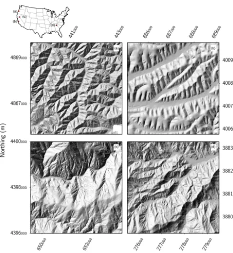
im-Figure 1.Map of the locations of each field site within the con-tinental USA with a shaded relief map of characteristic sections of each location’s topography. All coordinates are in UTM. (a) Oregon Coast Range, Oregon, UTM Zone 10N. (b) Gabilan Mesa, Califor-nia, UTM Zone 10N. (c) Northern Sierra Nevada, CaliforCalifor-nia, UTM Zone 10N. (d) Coweeta, North Carolina, UTM Zone 17N.
portant to define a channel network which correctly identi-fies the hillslope–fluvial transition, including the delineation of colluvial channels, which are often challenging to iden-tify using non-geomorphometric methods (Pelletier, 2013). Here we follow Pelletier (2013) and apply a Wiener filter (Wiener, 1949) to remove noise from the raw topographic data. Subsequently, channelized portions of the drainage net-work are identified based on a tangential curvature threshold (e.g., Pelletier, 2013). The appropriate curvature threshold is identified from the properties of its quantile–quantile plot (e.g., Lashermes et al., 2007; Passalacqua et al., 2010). These channelized patches of the landscape are combined by per-forming a connected-components analysis (He et al., 2008) which merges discreet patches of channel into a contiguous channel network. Following methods outlined in Grieve et al. (2016b), floodplain masks are also created and combined with this channel network, which separates the landscape into two domains: hillslopes and channels. This has the ef-fect of terminating hillslope traces when they reach a hollow or enter the floodplain, ensuring that the trace properties only reflect the hillslope domain and theE∗R∗measurements are not contaminated by sampling parts of the landscape which the nondimensional framework does not apply to.
If the channel network is incorrectly defined, some fluvial erosion could impact the correct measurement ofE∗R∗ val-ues. However, due to the number of individual measurements per landscape (>160 000 in each case) and the small num-ber of points on a landscape where such erroneous measure-ments could occur, such measuremeasure-ments will have little impact on landscape-scale trends, particularly when spatial averag-ing is applied.
4.2 Extraction of topographic parameters
All of the key measurements required to generateE∗R∗data can be extracted from high-resolution topography (Roering et al., 2007). Calculation ofE∗using Eq. (2) requires hills-lope length and hilltop curvature, and calculation ofR∗using Eq. (4) requires the relief and hillslope length to be measured from high-resolution topography.
Grieve et al. (2016b) measured hillslope length by generat-ing overland flow paths runngenerat-ing from hilltop to channel pix-els for every hilltop in a DEM, thereby generating a diverse range of measurements shown to characterize the range of hillslope properties inherent within a landscape. From these traces, each hilltop’s local relief is also measured by taking the difference between the elevation at the start (hilltop) and end (channel) of each trace. Finally, the hilltop curvature for each hilltop pixel is extracted following Hurst et al. (2012), whose techniques demonstrated that hilltop curvature scales linearly with erosion rate below hilltop gradients of 0.4. Cor-respondingly, we also sample the hilltop gradient (SHT) at
the start of each trace to allow data to later be filtered by this value. By using the methods outlined by Grieve et al. (2016b) we can generate a 4-tuple of information for each hilltop pixel in the landscape containing (LH, R, CHT, SHT).
4.3 Smoothing topographic parameters
In previous studies that generateE∗R∗ data, some form of smoothing has been employed to extract meaningful trends from the inherently noisy topographic data. Roering et al. (2007) hand-selected basins with uniform morphologies and minimal anthropogenic disturbance to measure topographic parameters from, effectively removing the majority of noise in the landscape and producing a small number of data points considered to be characteristic of their two steady-state land-scapes.
re-quired (see Sect. 5.1). These latter methods allowE∗R∗data to be used to interrogate transient landscapes, increasing the power of the method and providing a vital tool in the topo-graphic analysis of landscapes.
Here, we extract topographic parameters from raw topo-graphic data and smooth the resulting measurements, in ac-cordance with previous authors’ methods, firstly performing spatial averaging at a basin scale. The basins that are used to average the topographic parameters can be defined in an au-tomated manner to produce an average value over all basins of a given stream order, or a more user-defined approach can be undertaken to select basins manually in order to more closely replicate the work of Roering et al. (2007). Secondly the parameters can be averaged at a hillslope scale by us-ing the discrete hilltop patches generated usus-ing the technique outlined in Sect. 3.1. The data are filtered using the same constraints outlined in Hurst et al. (2012), removing hilltops with aSHT>0.4 or a patch size<50 m, with the additional
filtering of hillslope length and relief values below a user-defined threshold, typically 2–5 m for each parameter; this ensures that hilltops sampled are true hilltops and are not interfluves sitting adjacent to a basin outlet, which will not conform to models of hillslope sediment transport. The data are also returned to the user filtered, but not averaged, allow-ing users to explore the raw data to ensure that the smoothed data are a good reflection of the overall trends inherent in a landscape. Example basins and hilltop patches, used in the smoothing routines and the hillslope traces which produce the topographic measurements, are displayed in Fig. 2.
5 Processing the topographic data
Once the topographic data have been extracted, they are fil-tered to ensure that only data which conform to the nondi-mensional framework described by Roering et al. (2007) are used in any further analysis.
5.1 Filtering
The key filtering process which must be performed is the removal of any data points which have an SHT above 0.4.
This is the threshold gradient beyond which sediment flux no longer scales linearly with slope and thus hilltop curva-ture does not reflect erosion rate, forKvalues representative of published values for our field sites (Roering et al., 1999, 2007; Matmon et al., 2003; Hurst et al., 2012). Therefore data points with gradients above this value cannot be used in Eq. (2) as a proxy for erosion rate. Across all of the data sets, gradients which exceed 0.4 are removed from further analysis. In the case of the two spatially averaged data sets, individual hilltop pixels which exceed this threshold gradi-ent within a patch or basin are removed from the averaging process for each measurement, ensuring that no invalid data contribute to the final calculations. To ensure the validity of each basin average measurement, a count of the valid
pix-Figure 2.Map of a section of Gabilan Mesa, California (UTM Zone 10N), showing the examples of the spatial units used in the analysis ofE∗R∗data. Two second-order basins, colored green and purple, are bisected by a ridge with two hilltop patches, a large black patch and a smaller grey patch. From these patches, representative hills-lope traces, outlined in red, travel down the hillshills-lope and terminate at the channel network. Only 10 % of the total traces generated for this ridge have been plotted and other surrounding hilltop patches and their associated traces are not displayed, to aid clarity. Coordi-nates are in meters.
els contained within each basin following gradient filtering is performed and any basins with fewer valid measurements than a user-defined threshold can be removed from the anal-ysis. This threshold is typically equal to the minimum patch size used in Sect. 3.1 as this provides consistency between measurements.
5.2 Log binning
One method of non-spatial averaging of geomorphic data used effectively to generate slope–area plots (e.g., Tarolli and Dalla Fontana, 2009) is log binning. Such a method provides an opportunity to interrogate the data at a landscape scale while still removing the noise inherent in topographic mea-surements. EachE∗R∗pair is placed into evenly spaced bins in base 10 logarithmic space. The bin spacing is a function of the number of bins specified by the user, and the range of E∗values within the data set and its impact on interpretation of the data is considered in Sect. 6.2.3. To ensure that a valid number of data points make up each bin, a minimum bin size can also be specified by the user; this value will depend on the size and nature of the data set.
Mesa most of the data are expected to cluster around a single point (Roering et al., 2007), and so imposing evenly spaced bins in log space onto such data may construct an artificial trend. It is therefore recommended to consider the raw data in conjunction with the binned data to ensure that the trends in the data are valid.
5.3 Visualizing data
The software allows the user to plot any combination of the E∗R∗ data sets, facilitating the rapid generation of basin and landscape average data following Roering et al. (2007), hilltop-averaged and log-binned data following Hurst et al. (2012, 2013a), and raw data which have previously not been available. It is also possible to interrogate the raw measure-ments as a density plot, which more accurately conveys the trends in the raw data as in large landscapes many measure-ments share the same location inE∗R∗space. By allowing simple inter-comparisons between plotting methods it be-comes trivial to assess the most suitable data visualization techniques for a specific landscape.
6 Results and discussion
By using data from previous studies which utilize E∗R∗ analysis, it is possible to assess the ability of this software to reproduce existing results in addition to understanding how the varying techniques for smoothing the data, discussed in Sect. 4.3, can impact on the interpretation of the processes operating on a landscape. Four landscapes in the continental USA have been selected to evaluate the software: the Ore-gon Coast Range and Gabilan Mesa, used by Roering et al. (2007); Cascade Ridge, used by Hurst et al. (2012); and the Coweeta Hydrologic Laboratory (Fig. 1). High-resolution li-dar data are available from the National Center for Airborne Laser Mapping (NCALM) for each site and each site’s point cloud data have been gridded to 1 m resolution DEMs fol-lowing Kim et al. (2006) and accuracy information for each point cloud can be found in Appendix A.
6.1 Reproducing previous work
6.1.1 Oregon Coast Range and Gabilan Mesa
The Oregon Coast Range in Oregon, USA, is a steeply in-cised upland landscape with dense forest cover and a hu-mid climate (Roering et al., 1999), leading to frequent debris flows, which initiate in colluvial hollows (Stock and Dietrich, 2003). The forests of the Oregon Coast Range are dominated by hardwoods, such as Oregon maple (Acer macrophyllum), and coniferous forest such as Douglas fir (Pseudotsuga
men-ziesii) (Schmidt et al., 2001). Extensive work has been
car-ried out to estimate the uplift rate of the range using marine terrace data (Kelsey et al., 1996), and these estimates of uplift rate correspond to erosion rates measured using cosmogenic
radionuclides (e.g., Heimsath et al., 2001). This correspon-dence between uplift and erosion rate has been used to infer that the Oregon Coast Range is in steady state (e.g., Reneau and Dietrich, 1991; Roering et al., 2007).
Gabilan Mesa in California, USA, is part of the central Coast Ranges and has a semiarid Mediterranean climate with higher vegetation densities on northern slopes due to mi-croclimatic variations (Dohrenwend, 1978). The vegetation of Gabilan Mesa is characterized by a combinations of oak savannah containing blue oak (Quercus douglasii) and cha-parral shrubland containing chamise (Adenostoma
fascicu-latum) (Shreve, 1927). The landscape is very smooth with
a regular spacing of tributaries and valleys (Dohrenwend, 1978, 1979) and gentle transitions between hillslopes and channels, suggesting that diffusive processes dominate the transport of sediment on hillslopes (Roering et al., 2007). Hilltop curvature shows little variance across the landscape, and in conjunction with the regularity of valley spacing, this suggests that the landscape is in approximate topographic steady state (Roering et al., 2007; Perron et al., 2009).
Roering et al. (2007) estimated the topographic parameters LH,R, andCHT for the Oregon Coast Range and Gabilan
Mesa field sites. The characteristic hillslope length for each landscape was estimated by identifying the inflection point in a spline curve fitted though a plot of local slope against drainage area. This inflection point is considered to corre-spond to the transition between the hillslope and channel do-main in a landscape (Montgomery and Foufoula-Georgiou, 1993; Hancock and Evans, 2006; Tarolli and Dalla Fontana, 2009; Tarolli, 2014; Tseng et al., 2015).
Roering et al. (2007) estimated mean relief by calculating the mean of the differences between the maximum and min-imum elevation within a kernel of radius equal to the charac-teristic hillslope length for each point on the landscape. Hill-top curvature was sampled from manually defined hillHill-tops with a gradient below 0.05Scand averaged across each
land-scape. The critical gradient was calculated for the Oregon Coast Range to be 1.2 by Roering et al. (1999), and Roer-ing et al. (2007) assumed that this value is also correct for Gabilan Mesa.
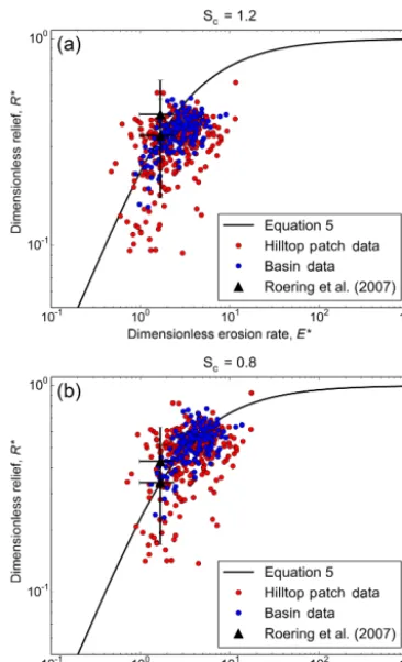
The data from Gabilan Mesa (Fig. 3a) reveal many hilltop patches which correspond closely to the predictedE∗R∗ val-ues from Roering et al. (2007). The data are predominantly clustered around a single point, showing strong agreement with observations that the landscape is in approximate steady state. However, the majority of the basin average data points and a considerable number of the hilltop patch data plot be-low the steady-state curve, which could be interpreted as ev-idence for topographic decay. However, the uniform hilltop curvatures and valley spacing, coupled with measurements of long-term erosion rates, suggest that this landscape is not undergoing topographic decay (Roering et al., 2007; Perron et al., 2009). An alternative explanation for the data falling below the steady-state curve is that anScvalue of 1.2 is too
Figure 3.Hilltop patch and basin average data for Gabilan Mesa plotted using a critical gradient of 1.2 (a) and 0.8 (b) alongside data from Roering et al. (2007) for the same location. Error bars are the standard error.
topographic parameters to estimate the critical gradient for this landscape as 0.8. By replotting these data using this re-visedSc, the data plot more closely to the steady-state curve
(Fig. 3b).
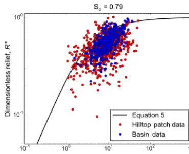
The Oregon Coast Range data are more tightly constrained than the Gabilan Mesa data (Fig. 4a), and have a similar range ofR∗values. However, as is the case for Gabilan Mesa, the majority of the data plot below the steady-state curve. This can be interpreted as evidence for topographic decay; however, due to the preponderance of evidence supporting a steady-state hypothesis for this landscape (e.g., Reneau and Dietrich, 1991; Roering et al., 2007), it is also possible that a critical gradient of 1.2 is too large in this location. By us-ing theScvalue of 0.79 constrained by Grieve et al. (2016b),
the data move closer to the steady-state curve (Fig. 4b). Us-ing this average Sc value several R∗ measurements exceed
1. This indicates that these hillslopes are too steep to sustain soil mantle in this landscape, which corresponds to field ob-servations of the Oregon Coast Range, where frequent shal-low landsliding is reported (e.g., Benda and Dunne, 1997; Montgomery et al., 1998) and where periodic wildfires ex-pose large (tens of square meters) patches of bedrock (Jack-son and Roering, 2009).
Figure 4.Hilltop patch and basin average data for the Oregon Coast Range plotted using a critical gradient of 1.2 (a) and 0.8 (b) along-side data from Roering et al. (2007) for the same location. Error bars are the standard error.
As acknowledged by Roering et al. (2007), extracting the relief from a moving window fails to capture the complete range of relief values in a landscape, resulting in an average value which dampens the true signal, reducingRin high re-lief landscapes such as the Oregon Coast Range. Our method of measuring relief of individual hillslope traces circumvents this problem.
The majority of the data points in Figs. 3 and 4 have larger E∗values than those from Roering et al. (2007). Grieve et al. (2016b) showed that estimating LH using slope–area plots
systematically underestimatesLHby as much as an order of
magnitude in some landscapes. Such an underestimate would reduce theE∗value for a landscape and explains the system-atic differences between this study and the results of Roering et al. (2007). The larger range of hilltop patch data highlights the range ofE∗R∗ values inherent in even a uniform land-scape which is in approximate topographic steady state.
6.1.2 Cascade Ridge
charac-teristic topographic form of this landscape is a smooth, low-relief relict surface which is heavily incised, creating steep canyons with an irregular spacing. The plateau surface is veg-etated with oak forest including California black oak
(Quer-cus kelloggii) and canyon live oak (Quer(Quer-cus chrysolepis) and
pine forest containing ponderosa pine (Pinus ponderosa), Douglas fir (Pseudotsuga menziesii), and sugar pine (Pinus
lambertiana), whereas the canyon is dominated by chaparal
vegetation such as manzanita (Arctostaphylos spp.) (Gabet et al., 2015; Milodowski et al., 2015a). These contrasting landscape morphologies have been shown to be eroding at different rates, with the plateau surfaces eroding an order of magnitude more slowly than the canyons (Riebe et al., 2000; Hurst et al., 2012). This produces a complex land-scape exhibiting a range of erosion rates influenced by cli-mate and tectonic signals, which is not in topographic steady state (Riebe et al., 2000; Stock et al., 2004; Hurst et al., 2012; Gabet et al., 2015).
Cascade ridge is a more morphologically complex land-scape than the Oregon Coast Range or Gabilan Mesa; corre-spondingly, theE∗R∗data for this landscape are predicted to plot along the steady-state curve at a broad range of E∗ values, as was demonstrated by Hurst et al. (2012). Using anSc value of 0.8, as proposed by Hurst et al. (2012),
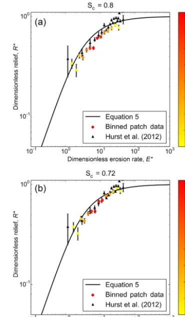
pro-duces data spanning a much wider portion of E∗R∗ space than the data for the steady-state landscapes of Gabilan Mesa and the Oregon Coast Range (Fig. 5a). The binned hilltop patch data show good agreement with the data from Hurst et al. (2012), spanning a similar range ofE∗values with the steady-state curve falling within the standard error of each bin. This supports observations of a range of erosion rates and landscape morphologies and highlights the utility of this method in gaining a first-order approximation of the tectonic and erosional setting of a landscape where no field data are available.
At the Cascade Ridge site, Grieve et al. (2016b) estimated Sc to be 0.72, calculated from topographic parameters.
Us-ing this value there is little change in the trends in the data (Fig. 5b), most of the points now fall above the line and at high values ofE∗, and more data points haveR∗ values in excess of 1. These highR∗ values are consistent with field observations of this transient landscape wherein rapid valley downcutting may decouple hillslopes from the channel net-work (Milodowski et al., 2015b) and drive shallow landslid-ing. In a complex landscape such as Cascade Ridge, which is known to have a broad range of erosion rates and hills-lope morphologies, a landscape averageScvalue will regress
towards the mean. Consequently, as more of the landscape is covered by the low-gradient plateau than the steeper canyons, theScvalue of 0.72 does not reflect the parts of the landscape
with largerE∗R∗values, which may fall closer to the value of 0.8 used by Hurst et al. (2012).
Figure 5.Binned hilltop patch data spanning a wide range ofE∗
values generated using a critical gradient of 0.8 (a) and 0.72 (b) alongside data from Hurst et al. (2012) for the same location. Error bars are the standard error of the data. Error bars from Hurst et al. (2012) are generated from the original data.
6.1.3 Coweeta
The Coweeta Hydrologic Laboratory is in the southern Ap-palachian Mountains in North Carolina, USA, and is a densely vegetated landscape which exhibits classic ridge and hollow topography (Hales et al., 2012). Such topography pro-duces many source areas for shallow landslides in colluvial hollows, which are triggered by high-intensity storms con-nected to hurricanes (Swift Jr. et al., 1988). The vegetation at Coweeta is a mix of shrubs, such as Rhododendron
max-ima, and northern hardwood forest, the distribution of which
is controlled by wildfires, which in many cases are managed through human intervention (Hales et al., 2009). It is debated whether the southern Appalachians are in topographic steady state, as there is little tectonic activity, yet there is a large amount of relief preserved across the range (Baldwin et al., 2003; Matmon et al., 2003; Gallen et al., 2011, 2013).
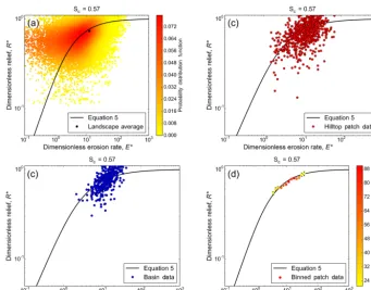
Figure 6.Comparison of the different methods which can be used to visualizeE∗R∗from Coweeta, using a critical gradient of 0.57. (a) Raw data colored by the density of points inE∗R∗space alongside the landscape average value. Error bars plot inside the data point. (b) Data averaged over hilltop patches. (c) Data averaged over second-order drainage basins. (d) Hilltop patch data placed into logarithmically spaced bins. Error bars are the standard error.
signals. Figure 6 outlines the range of methods which can be used to interpretE∗R∗data. As in Sects. 6.1.1 and 6.1.2 the critical gradient used is taken from Grieve et al. (2016b). The raw data in Fig. 6a show the range of reliefs observed in the southern Appalachians. The landscape medianE∗R∗ value falls within the zone of maximum probability density; this highlights the level of noise inherent in high-resolution topographic data when interrogating them in E∗R∗ space, outlining the requirement to smooth or bin the data in order to extract meaningful information from them.
Comparing the data in Fig. 6b and 6c to data for steady-state landscapes such as Gabilan Mesa or the Oregon Coast Range, they show similar levels of clustering, with the loca-tion of the cluster of patch and basin average values corre-sponding with the Oregon Coast Range data (Fig. 4). This corresponds well to field observations of hillslope morphol-ogy in these two locations, with planar hillslopes and fre-quent shallow landsliding reported (Benda and Dunne, 1997; Montgomery et al., 1998; Roering et al., 1999), and this clustering suggests that there is less spatial variation in ero-sion rate in Coweeta than in Cascade Ridge, an assertion supported by measured erosion rates from both locations (e.g., Riebe et al., 2000; Matmon et al., 2003; Hales et al., 2012; Hurst et al., 2012). Figure 6d shows the binned data for Coweeta and highlights the smaller range of E∗ values for this landscape when compared to Cascade Ridge. It also
draws attention to the need to analyzeE∗R∗data using nu-merous methods to avoid an incorrect interpretation, as dis-cussed in Sect. 5.2.
The Coweeta E∗R∗ data cluster around a point on the steady-state curve, and it could be concluded that this land-scape is in approximate steady state. However, the value of Scused in Fig. 6 is significantly smaller than any previously
publishedScvalue. Field observations of Coweeta reveal that
many channels are alluviated and such deposition at the base of hillslopes will alter the mean properties of a hillslope and move its idealized profile away from the model hillslopes de-fined by Roering et al. (2007). As a valley fills with sediment, the hillslope relief will be reduced more rapidly than other hillslope properties, due to the difference between rates of hillslope and channel response to forcing (Hurst et al., 2012). Such a reduction in relief will reduceR∗, resulting in a re-duced best-fitScvalue. Such an alteration of mean hillslope
properties could explain the considerable underestimation of the critical gradient when it is constrained through hillslope length–relief relationships.
The Oregon Coast Range, a broadly similar landscape to Coweeta, based on the range ofE∗values, general landscape morphology and observations of sediment transport pro-cesses, has a critical gradient of 0.79 (Grieve et al., 2016b). This value is similar to theScof many other landscapes
Figure 7.Hilltop patch data from Coweeta plotted using the higher
Scvalue of 0.79, demonstrating that the majority of the hillslopes in this landscape plot below the steady-state curve when using a larger critical gradient.
as such we use this value to explore the patterns ofE∗R∗in Coweeta when a larger critical gradient which more closely resembles predicted values for other landscapes is employed. In such a case the majority of the data plot below the steady-state curve (Fig. 7). Hurst et al. (2013a) observedE∗R∗data plotting below the steady-state curve, along the Dragon’s Back pressure ridge, where these sections of the landscape are understood to be topographically decaying following a pulse of uplift. If thisScis correct it could lend support to the
idea of a Miocene rejuvenation of topography in the south-ern Appalachians (Gallen et al., 2013) followed by a period of gradual topographic decay into the present. However, the nature of sediment transport in Coweeta may not be best con-strained using Eq. (1), as modeling work performed by Mudd (2016) suggests that a deviation of this magnitude from the steady-state curve indicates that a landscape is not undergo-ing pure nonlinear sediment flux.
6.2 Sensitivity analysis of averaging methods
Several of the techniques utilized to average the rawE∗R∗ data have free parameters, the selection of which can influ-ence the final results. In the following section we explore the influence that averaging technique, minimum patch and basin area, basin stream order, and binning parameters can have on the interpretation ofE∗R∗data.
6.2.1 Averaging methods
As outlined in Sect. 4.3, the topographic parameters, LH, R, CHT, andSHT, must be smoothed in order to extract
meaningful trends from the inherently noisy signal. The main technique for performing this smoothing is to spatially aver-age the data over either hilltop patches or drainaver-age basins. These averages can be computed as either the mean or the median of each spatial area. Figure 8 presents a comparison
Figure 8.Comparison between hilltop patch values generated using a spatial mean (a) and a spatial median (b) for the Oregon Coast Range.
between hilltop patch data computed using means and me-dians for the Oregon Coast Range, showing little change be-tween the measurements using the two techniques. Because there is little difference between the two methods, we use median values throughout this paper, as this ensures that any extreme values will have a lesser impact on landscape-scale metrics.
6.2.2 Spatial averaging parameters
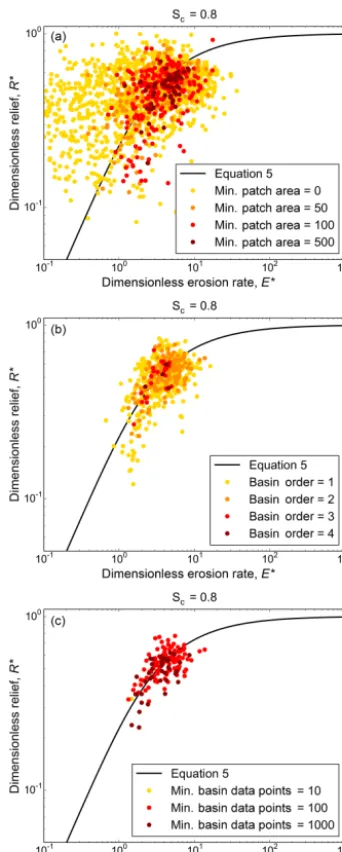
Figure 9.Comparison of the influence of changing spatial averag-ing method on the interpretation ofE∗R∗data for Gabilan Mesa.
(a) Variations in the minimum patch area threshold from 0 (no
threshold) to 500 pixels highlighting the reduction in noise when a minimum patch area is applied. (b) Increasing the basin steam or-der, which reduces variance in the data, as bigger basins are sets containing basins of smaller orders, dampening any extreme val-ues. (c) Variations in the minimum basin pixels threshold. Outly-ing basins have very few data points, so they are influenced more strongly by single atypical values.
patch to ensure that a small number of measurements do not have too large an impact on the interpretation of the data.
The technique in Sect. 3.1 has no method to limit the max-imum size of the hilltop patches, as the aim is to find spa-tially contiguous zones of hilltop and artificially breaking these patches may result in oversampling some sections of a landscape. Large patches make up a very small proportion
of the total population of patches and correspondingly do not have a large impact on the overall trends in an individual data set.
The stream order of the basin used to generate basin av-erage values will also have an influence on the interpretation of the results. Grieve et al. (2016b) used second-order basins to generate basin average topographic parameters as this or-der generated a large number of basins which all had a large enough area to generate numerous data points per basin, ef-fectively sampling as much of the landscape as possible. Fig-ure 9b shows the effect of increasing the stream order of the basins used in Coweeta from first to fourth order. As each increasing order basin can be considered a set containing the previous order basins, the basin average points all plot in very similar locations inE∗R∗space, suggesting that in-creasing basin order may be a useful method of smoothing basin average data in noisy landscapes. However, this comes with the limitation that, as the basin order increases, the num-ber of basins in a landscape decreases, resulting in fewer data points representing larger spatial areas and the possible homogenization of topographic signals occurring at spatial scales smaller than the average basin area.
The number of valid data points contained within a basin used to generate an average value is another free parameter that the user must set. As with the hilltop patch area, selecting a sensible value is important to ensure that each basin aver-age data point corresponds to the basin as a whole and not just a spatial subset. As the threshold is increased, outlying basins are removed (Fig. 9c), indicating that many outlying data points are generated by a small number of irregular hill-slopes in otherwise typical basins. However, if the threshold is too large, too many basins will be excluded. In order to ensure consistency between spatial averaging techniques it is recommended that the minimum number of pixels in a basin be kept equal with the minimum patch area.
6.2.3 Log bin parameters
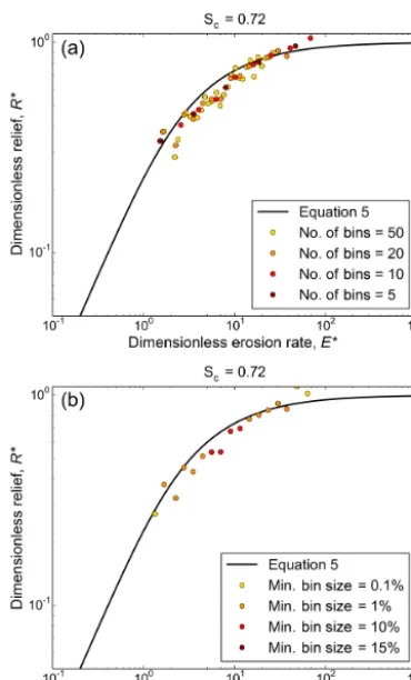
When computing logarithmically spaced bins there are two free parameters, the number of bins (equivalent to the bin width) and the minimum number of data points which must fall within a bin for the binned point to be valid. Figure 10a highlights the influence of changing the number of bins on the interpretation of the Cascade Ridge data. If the number of bins are too low, it becomes difficult to identify a trend in the data as the nature of a landscape can vary consider-ably across large ranges ofE∗, and by homogenizing these measurements a transient signal can be lost.
Figure 10.Comparison of the influence of binning parameters on the interpretation ofE∗R∗data for Cascade Ridge. (a) Varying the number of bins used, equivalent to the bin width inE∗space. As the number of bins reduces it becomes harder to identify patterns in the data, and as the number of bins increases, the number of data points in each bin reduces, thereby reducing the power of the binning tech-nique. (b) Varying the minimum number of data points required in a basin. As this value increases, fewer points are preserved, which compresses the range of the data and can obscure the observation of an erosional gradient. Too small a threshold can result in bins con-taining very few values which do not represent the landscape as a whole.
data are sparser. We have found that using 20 bins reaches a good compromise between data density and data smoothing, and corresponds well with the 21 bins used by Hurst et al. (2012), where no filtering was performed based on bin size.
The minimum size of each bin can also have an impact on the final interpretation of the data. If no threshold is ap-plied, some bins can contain a single value, while others can contain hundreds of values, which makes interpreting the data difficult as one cannot be sure of the robustness of each binned value. If the threshold is placed too high, then valid data will not be included in the final analysis and the inter-pretation of a landscape’s evolution could be incorrect. Fig-ure 10b highlights this issue using data from Cascade Ridge at a range of bin size thresholds, identified as percentages of the total data set size. We have found that using a minimum
bin size of 1–5 % of the total data set ensures a good binning result.
6.3 ConstrainingSc
Landscapes which are in topographic steady state should plot at a single location on the curve described by Eq. (5). In principle this would mean that an erosion gradient would be required in order to constrain Sc, by fitting the data to the
steady-state curve. However, as observed in Figs. 3 and 4, even in idealized steady-state landscapes, there is still con-siderable variability in the E∗R∗ data. This variability is consistent with patterns of dynamic reorganization of low-order drainage basins within models of steady-state land-scapes performed by Reinhardt and Ellis (2015). Therefore, it becomes possible to estimate the critical gradient of the nonlinear sediment flux law (Eq. 1) for a landscape without a strong erosion gradient, usingE∗R∗data.
As with previous analyses, the raw data must be spatially averaged in order to reduce the level of noise present in E∗R∗space before an estimate ofSccan be made. The
op-timal value ofScis estimated using a nonlinear least-squares
method (Jones et al., 2001) which computes the sum of the square of the deviation between each measuredE∗R∗value and the value predicted by Eq. (5). This calculation is per-formed for a range of critical gradients until theScwith the
lowest corresponding deviation from the steady-state curve is found.
The accuracy of this optimized Sc value is constrained
through bootstrapping the optimization procedure. The data are sampled with replacement to generate 100 000 data sets, consisting of values randomly drawn from the population of patch or basin average data. For each of these sampled data sets the optimal value ofSc which minimizes the error
be-tween the data and the steady-state curve is calculated. The finalScvalue for each landscape is the mean value of these
100 000 iterations, with a 95 % confidence interval.
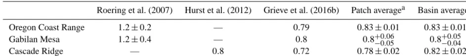
Table 1 contains estimates of the critical gradient gener-ated using both basin and patch average values alongside previously published values for Cascade Ridge, the Oregon Coast Range, and Gabilan Mesa. The predicted patch and basin average values for Gabilan Mesa and the Oregon Coast Range are similar to those published by Grieve et al. (2016b). This method of estimating the best-fitScwill produce an
av-erage value representative of the maximum probability den-sity ofScvalues for a landscape, whereas the method ofSc
estimation employed by Roering et al. (1999) can better be considered as the maximumScvalue for a landscape Grieve
et al. (2016b).
The data for Cascade Ridge show better agreement with the value used by Hurst et al. (2012), which was also de-rived usingE∗R∗data, than the lower estimate from Grieve et al. (2016b). The pair ofScvalues calculated for each
Table 1.Previously publishedScvalues alongside the values generated from the best fit to the steady-state curve for the patch and basin average data.
Roering et al. (2007) Hurst et al. (2012) Grieve et al. (2016b) Patch averagea Basin averageb
Oregon Coast Range 1.2±0.2 — 0.79 0.83±0.01 0.83±0.01 Gabilan Mesa 1.2±0.4 — 0.8 0.8+0.06−0.05 0.8+0.05−0.04 Cascade Ridge — 0.8 0.72 0.78±0.02 0.82±0.02
aCalculated as the value which minimizes the sum of the squared residuals to the steady-state line for the patch average data. Error is the 95 % confidence interval
generated by bootstrapping the calculation 100 000 times.
bAs above but using basin average data.
data averaging. However, the scale of spatial averaging has been demonstrated to have an impact on the interpretation of E∗R∗ data and thus care must be taken to select appropri-ate methods of spatial averaging and data processing in order to ensure that results generated are not simply a function of user-defined parameters.
The similarity of the average Sc values obtained using
the bootstrapping procedure across three diverse landscapes highlights the presence of a distribution ofE∗R∗values ex-isting for each landscape, and the nature of an average Sc
measurement. Such a distribution occurs due to local vari-ations in topography, process, and material properties, and similarities can be drawn between the results presented in Table 1 and other similar studies (DiBiase et al., 2010; Hurst et al., 2012).
The values ofScconstrained using this bootstrapping
pro-cedure are similar to those derived from the relationship be-tween hillslope length and relief demonstrated by Grieve et al. (2016b); however, there is no need to estimate mate-rial properties such as the soil and rock density and thus this method provides an independent constraint onSc. However,
the computational expense of bootstrapping theScfitting
cal-culations from theE∗R∗data is very high, when contrasted with the estimation ofScusingLH-Rrelationships presented
by Grieve et al. (2016b). Additionally, using this bootstrap-ping method in landscapes which do not plot on the steady-state curve in E∗R∗ space can yield an incorrectSc value
with a low error estimate. Consequently, we recommend es-timating the critical gradient of a landscape using this method and the method outlined in Grieve et al. (2016b), when field data are available, in order to best constrain the critical gra-dient of a landscape. However, careful consideration of the differences between a maximumScand a best-fit-derived
av-erageScshould be undertaken to ensure that a valid
geomor-phic interpretation of a landscape is employed.
7 Conclusions
We present a software package which automates the extrac-tion and processing of high-resoluextrac-tion topographic data to generate nondimensional erosion rate and relief measure-ments. Topographic data can be averaged at a hilltop scale
by generating unique hilltop patches or can be averaged over drainage basins automatically extracted from the channel network. Alongside the raw data, these spatially averaged data sets are shown to reproduce the findings of previous studies. In steady-state landscapes such as the Oregon Coast Range and Gabilan Mesa,E∗R∗data plot in a cluster around a single point on the steady-state curve, supporting the con-clusions drawn in previous studies (Roering et al., 2007), and in Cascade Ridge, a transient erosion signal similar to that identified by Hurst et al. (2012) is observed. This technique is also tested on a landscape in the southern Appalachian Mountains, with the results suggesting that topography is de-caying, supporting models of Miocene topographic rejuvena-tion proposed by Gallen et al. (2013). These results, along-side the ability to reproduce previous work, emphasize the value of this software to the geomorphology community as, until now, there has been no clear framework within which to produce nondimensional erosion rate and relief measure-ments.
The average critical gradient used in Eq. (1) is also con-strained for three of the studied landscapes, with the values falling within expected ranges. However, due to the noise in-herent in this form of analysis and the challenges of evaluat-ing the goodness of fit between such noisy data and a model, it is recommended that other methods to constrainSc using
the same raw data be utilized instead. Finally, the influence of free parameters on the final interpretation of the data are explored, providing the user clear guidance on how to se-lect parameters which control the level of smoothing or bin-ning performed on the topographic data. The most significant of which are the minimum patch and basin size thresholds which must be carefully selected to balance smoothing the data with preserving landscape-scale trends.
Data availability
Appendix A: Topographic metadata
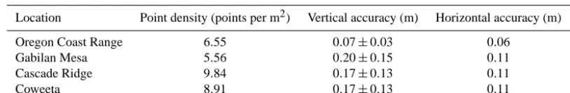
This table provides the accuracy information for the four point clouds used to generate the 1 m resolution topographic data used in this study. This information is compiled from metadata available from http://OpenTopography.org.
Table A1.Lidar point cloud metadata.
Location Point density (points per m2) Vertical accuracy (m) Horizontal accuracy (m)
Oregon Coast Range 6.55 0.07±0.03 0.06
Gabilan Mesa 5.56 0.20±0.15 0.11
Cascade Ridge 9.84 0.17±0.13 0.11
Author contributions. S. W. D. Grieve developed the data anal-ysis and visualization code and performed the data analanal-ysis. S. W. D. Grieve, S. M. Mudd, M. D. Hurst, and D. T. Milodowski wrote the topographic analysis code. S. W. D. Grieve wrote the manuscript with contributions from S. M. Mudd, M. D. Hurst, and D. T. Milodowski.
Acknowledgements. The topographic data used in this paper are freely available from http://www.opentopography.org. All the code used in this analysis is open source and can be downloaded from https://github.com/LSDtopotools/LSDTT_Hillslope_Analysis, http://github.com/sgrieve/ER_Star/, and http://github.com/sgrieve/ ER_Star_Figs/. The data used to generate all the plots are pub-lished as “A nondimensional relief framework: data” (Grieve et al., 2016a). S. W. D. Grieve is supported by NERC grant NE/J009970/1. S. M. Mudd is supported by US Army Research Office contract number W911NF-13-1-0478. D. T. Milodowski is supported by NERC grants NE/152830X/1 and J500021/1, in addition to the Harkness Award from the University of Cambridge. This paper is published with the permission of the Executive Director of the British Geological Survey and was supported in part by the Climate and Landscape Change research program at the British Geological Survey. We thank Fiona Clubb for discussions and advice which shaped the final form of the manuscript. The manuscript was improved through the detailed reviews provided by Jon Pelletier; an anonymous reviewer; and the associate editor, Susan Conway.
Edited by: S. Conway
References
Anders, A. M., Roe, G. H., Montgomery, D. R., and Hallet, B.: In-fluence of precipitation phase on the form of mountain ranges, Geology, 36, 479–482, doi:10.1130/G24821A.1, 2008.
Andrews, D. J. and Bucknam, R. C.: Fitting degradation of shoreline scarps by a nonlinear diffusion model, J. Geophys. Res.-Sol. Ea., 92, 12857–12867, doi:10.1029/JB092iB12p12857, 1987. Baldwin, J. A., Whipple, K. X., and Tucker, G. E.: Implications of
the shear stress river incision model for the timescale of postoro-genic decay of topography, J. Geophys. Res.-Sol. Ea., 108, 2158, doi:10.1029/2001JB000550, 2003.
Benda, L. and Dunne, T.: Stochastic forcing of sediment supply to channel networks from landsliding and debris flow, Water Resour. Res., 33, 2849–2863, https://www.wou.edu/las/physci/ taylor/andrews_forest/refs/benda_dunne_1997.pdf, 1997. Binnie, S. A., Phillips, W. M., Summerfield, M. A., and
Fi-field, L. K.: Tectonic uplift, threshold hillslopes, and denuda-tion rates in a developing mountain range, Geology, 35, 743–746, doi:10.1130/G23641A.1, 2007.
Booth, A. M., Roering, J. J., and Rempel, A. W.: Topographic sig-natures and a general transport law for deep-seated landslides in a landscape evolution model, J. Geophys. Res.-Earth, 118, 603– 624, doi:10.1002/jgrf.20051, 2013.
Braun, J., Heimsath, A. M., and Chappell, J.: Sediment transport mechanisms on soil-mantled hillslopes, Geology, 29, 683–686,
doi:10.1130/0091-7613(2001)029<0683:STMOSM>2.0.CO;2, 2001.
Champagnac, J.-D., Molnar, P., Sue, C., and Herman, F.: Tecton-ics, climate, and mountain topography, J. Geophys. Res.-Sol. Ea., 117, B02403, doi:10.1029/2011JB008348, 2012.
Clarke, B. A. and Burbank, D. W.: Bedrock fracturing, threshold hillslopes, and limits to the magnitude of bedrock landslides, Earth Planet. Sc. Lett., 297, 577–586, doi:10.1016/j.epsl.2010.07.011, 2010.
Clarke, B. A. and Burbank, D. W.: Quantifying bedrock-fracture patterns within the shallow subsurface: Implications for rock mass strength, bedrock landslides, and erodibility, J. Geophys. Res.-Earth, 116, F04009, doi:10.1029/2011JF001987, 2011. Clubb, F. J., Mudd, S. M., Milodowski, D. T., Hurst, M. D., and
Slater, L. J.: Objective extraction of channel heads from high-resolution topographic data, Water Resour. Res., 50, 4283–4304, doi:10.1002/2013WR015167, 2014.
Culling, W. E. H.: Analytical Theory of Erosion, The Journal of Geology, 68, 336–344, 1960.
DiBiase, R. A., Whipple, K. X., Heimsath, A. M., and Ouimet, W. B.: Landscape form and millennial erosion rates in the San Gabriel Mountains, CA, Earth Planet. Sc. Lett., 289, 134–144, doi:10.1016/j.epsl.2009.10.036, 2010.
DiBiase, R. A., Heimsath, A. M., and Whipple, K. X.: Hillslope response to tectonic forcing in threshold landscapes, Earth Surf. Proc. Land., 37, 855–865, doi:10.1002/esp.3205, 2012. Dietrich, W. E., Bellugi, D. G., Sklar, L. S., Stock, J. D.,
Heim-sath, A. M., and Roering, J. J.: Geomorphic Transport Laws for Predicting Landscape form and Dynamics, in: Prediction in Ge-omorphology, edited by Wilcock, P. R. and Iverson, R. M., 103– 132, American Geophysical Union, Washington, DC, 2003. Dillencourt, M. B., Samet, H., and Tamminen, M.: A
Gen-eral Approach to Connected-component Labeling for Arbitrary Image Representations, J. ACM, 39, 253–280, doi:10.1145/128749.128750, 1992.
Dohrenwend, J. C.: Systematic valley asymmetry in the cen-tral California Coast Ranges, Geol. Soc. Am. Bull., 89, 891– 900, doi:10.1130/0016-7606(1978)89<891:SVAITC>2.0.CO;2, 1978.
Dohrenwend, J. C.: Morphologic Analysis of Gabilan Mesa by Iterative Contour-Generalization: An Improved Method of Ge-omorphic Cartographic Analysis, SEPM Pacific Coast Pale-ogeography Field Guide #4, Menlo Park, California, 83–87, available at: http://archives.datapages.com/data/pac_sepm/025/ 025001/pdfs/83.htm, 1979.
Foufoula-Georgiou, E., Ganti, V., and Dietrich, W. E.: A nonlo-cal theory of sediment transport on hillslopes, J. Geophys. Res.-Earth, 115, F00A16, doi:10.1029/2009JF001280, 2010. Furbish, D. J. and Fagherazzi, S.: Stability of creeping soil and
im-plications for hillslope evolution, Water Resour. Res., 37, 2607– 2618, doi:10.1029/2001WR000239, 2001.
Furbish, D. J. and Roering, J. J.: Sediment disentrainment and the concept of local versus nonlocal transport on hillslopes, J. Geo-phys. Res.-Earth, 118, 937–952, doi:10.1002/jgrf.20071, 2013. Gabet, E. J., Pratt-Sitaula, B. A., and Burbank, D. W.: Climatic
con-trols on hillslope angle and relief in the Himalayas, Geology, 32, 629–632, doi:10.1130/G20641.1, 2004.
re-golith thickness along a ridgeline in the Sierra Nevada, Califor-nia, Earth Surf. Proc. Land., 1779–1790, doi:10.1002/esp.3754, 2015.
Gallen, S. F., Wegmann, K. W., Frankel, K. L., Hughes, S., Lewis, R. Q., Lyons, N., Paris, P., Ross, K., Bauer, J. B., and Witt, A. C.: Hillslope response to knickpoint migration in the Southern Appalachians: implications for the evolution of post-orogenic landscapes, Earth Surf. Proc. Land., 36, 1254–1267, doi:10.1002/esp.2150, 2011.
Gallen, S. F., Wegmann, K. W., and Bohnenstieh, D. R.: Miocene rejuvenation of topographic relief in the southern Appalachians, GSA Today, 23, 4–10, doi:10.1130/GSATG163A.1, 2013. Grieve, S. W. D., Mudd, S. M., Hurst, M. D., and Milodowski, D. T.:
A nondimensional relief framework: data, dataset, University of Edinburgh, School of GeoSciences, doi:10.7488/ds/1366, 2016a. Grieve, S. W. D., Mudd, S. M., and Hurst, M. D.: How long is a hillslope?, Earth Surf. Proc. Land., doi:10.1002/esp.3884, 2016b. Hales, T. C., Ford, C. R., Hwang, T., Vose, J. M., and Band, L. E.: Topographic and ecologic controls on root reinforcement, J. Geophys. Res.-Earth, 114, F03013, doi:10.1029/2008JF001168, 2009.
Hales, T. C., Scharer, K. M., and Wooten, R. M.: Southern Ap-palachian hillslope erosion rates measured by soil and de-trital radiocarbon in hollows, Geomorphology, 138, 121–129, doi:10.1016/j.geomorph.2011.08.030, 2012.
Hancock, G. R. and Evans, K. G.: Channel head location and characteristics using digital elevation models, Earth Surf. Proc. Land., 31, 809–824, doi:10.1002/esp.1285, 2006.
He, L., Chao, Y., and Suzuki, K.: A Run-Based Two-Scan La-beling Algorithm, IEEE T. Image Processing, 17, 749–756, doi:10.1109/TIP.2008.919369, 2008.
He, L.-F., Chao, Y.-Y., and Suzuki, K.: An Algorithm for Connected-Component Labeling, Hole Labeling and Euler Number Computing, J. Comput. Sci. Technol., 28, 468–478, doi:10.1007/s11390-013-1348-y, 2013.
Heimsath, A. M., Dietrich, W. E., Nishiizumi, K., and Finkel, R. C.: Stochastic processes of soil production and transport: erosion rates, topographic variation and cosmogenic nuclides in the Oregon Coast Range, Earth Surf. Proc. Land., 26, 531–552, doi:10.1002/esp.209, 2001.
Heimsath, A. M., Furbish, D. J., and Dietrich, W. E.: The illusion of diffusion: Field evidence for depth-dependent sediment trans-port, Geology, 33, 949–952, doi:10.1130/G21868.1, 2005. Hilley, G. E. and Arrowsmith, J. R.: Geomorphic response to uplift
along the Dragon’s Back pressure ridge, Carrizo Plain, Califor-nia, Geology, 36, 367–370, doi:10.1130/G24517A.1, 2008. Hurst, M. D., Mudd, S. M., Walcott, R., Attal, M., and Yoo,
K.: Using hilltop curvature to derive the spatial distribu-tion of erosion rates, J. Geophys. Res.-Earth, 117, F02017, doi:10.1029/2011JF002057, 2012.
Hurst, M. D., Mudd, S. M., Attal, M., and Hilley, G.: Hillslopes Record the Growth and Decay of Landscapes, Science, 341, 868– 871, doi:10.1126/science.1241791, 2013a.
Hurst, M. D., Mudd, S. M., Yoo, K., Attal, M., and Walcott, R.: In-fluence of lithology on hillslope morphology and response to tec-tonic forcing in the northern Sierra Nevada of California, J. Geo-phys. Res.-Earth, 118, 832–851, doi:10.1002/jgrf.20049, 2013b. Jackson, M. and Roering, J. J.: Post-fire geomorphic re-sponse in steep, forested landscapes: Oregon Coast
Range, USA, Quaternary Sci. Rev., 28, 1131–1146, doi:10.1016/j.quascirev.2008.05.003, 2009.
Jones, E., Oliphant, T., and Peterson, P.: SciPy: Open source sci-entific tools for Python, available at: http://www.scipy.org/ (last access: 8 March 2015), 2001.
Kelsey, H. M., Ticknor, R. L., Bockheim, J. G., and Mitchell, E.: Quaternary upper plate deformation in coastal Ore-gon, Geol. Soc. Am. Bull., 108, 843–860, doi:10.1130/0016-7606(1996)108<0843:QUPDIC>2.3.CO;2, 1996.
Kim, H., Arrowsmith, J., Crosby, C. J., Jaeger-Frank, E., Nandigam, V., Memon, A., Conner, J., Baden, S. B., and Baru, C.: An efficient implementation of a local binning algorithm for dig-ital elevation model generation of LiDAR/ALSM dataset, in: AGU Fall Meeting Abstracts, vol. 1, p. 0921, San Francisco, http://adsabs.harvard.edu/abs/2006AGUFM.G53C0921K, 2006. Korup, O.: Rock type leaves topographic signature in landslide-dominated mountain ranges, Geophys. Res. Lett., 35, L11402, doi:10.1029/2008GL034157, 2008.
Lashermes, B., Foufoula-Georgiou, E., and Dietrich, W. E.: Channel network extraction from high resolution topography using wavelets, Geophysical Research Letters, 34, L23S04, doi:10.1029/2007GL031140, 2007.
Lumia, R., Shapiro, L., and Zuniga, O.: A new connected components algorithm for virtual memory computers, Com-puter Vision, Graphics, and Image Processing, 22, 287–300, doi:10.1016/0734-189X(83)90071-3, 1983.
Matmon, A., Bierman, P. R., Larsen, J., Southworth, S., Pavich, M., and Caffee, M.: Temporally and spatially uni-form rates of erosion in the southern Appalachian Great Smoky Mountains, Geology, 31, 155–158, doi:10.1130/0091-7613(2003)031<0155:TASURO>2.0.CO;2, 2003.
McKean, J. A., Dietrich, W. E., Finkel, R. C., Southon, J. R., and Caffee, M. W.: Quantification of soil production and downs-lope creep rates from cosmogenic 10Be accumulations on a hillslope profile, Geology, 21, 343–346, doi:10.1130/0091-7613(1993)021<343:QOSPAD>2.3.CO;2, 1993.
Milodowski, D. T., Mudd, S. M., and Mitchard, E. T.: Erosion rates as a potential bottom-up control of forest structural char-acteristics in the Sierra Nevada Mountains, Ecology, 96, 31–38, http://www.esajournals.org/doi/abs/10.1890/14-0649.1, 2015a. Milodowski, D. T., Mudd, S. M., and Mitchard, E. T. A.:
Topographic roughness as a signature of the emergence of bedrock in eroding landscapes, Earth Surf. Dynam., 3, 483–499, doi:10.5194/esurf-3-483-2015, 2015b.
Montgomery, D. R. and Foufoula-Georgiou, E.: Channel network source representation using digital elevation models, Water Re-sour. Res., 29, 3925–3934, doi:10.1029/93WR02463, 1993. Montgomery, D. R., Sullivan, K., and Greenberg, H. M.: Regional
test of a model for shallow landsliding, Hydrol. Process., 12, 943–955, 1998.
Mudd, S. M.: Detection of transience in eroding landscapes, Earth Surf. Proc. Land., doi:10.1002/esp.3923, 2016.
Mudd, S. M. and Furbish, D. J.: Influence of chemical denudation on hillslope morphology, J. Geophys. Res.-Earth, 109, F02001, doi:10.1029/2003JF000087, 2004.
Passalacqua, P., Do Trung, T., Foufoula-Georgiou, E., Sapiro, G., and Dietrich, W. E.: A geometric framework for channel network extraction from lidar: Nonlinear diffusion and geodesic paths, J. Geophys. Res.-Earth, 115, F01002, doi:10.1029/2009JF001254, 2010.
Pelletier, J. D.: A robust, two-parameter method for the extraction of drainage networks from high-resolution digital elevation models (DEMs): Evaluation using synthetic and real-world DEMs, Wa-ter Resour. Res., 49, 75–89, doi:10.1029/2012WR012452, 2013. Perron, J. T., Kirchner, J. W., and Dietrich, W. E.: Formation of evenly spaced ridges and valleys, Nature, 460, 502–505, doi:10.1038/nature08174, 2009.
Reinhardt, L. and Ellis, M. A.: The emergence of topo-graphic steady state in a perpetually dynamic self-organized critical landscape, Water Resour. Res., 51, 4986–5003, doi:10.1002/2014WR016223, 2015.
Reneau, S. L. and Dietrich, W. E.: Erosion rates in the southern ore-gon coast range: Evidence for an equilibrium between hillslope erosion and sediment yield, Earth Surf. Proc. Land., 16, 307–322, doi:10.1002/esp.3290160405, 1991.
Riebe, C. S., Kirchner, J. W., Granger, D. E., and Finkel, R. C.: Erosional equilibrium and disequilibrium in the Sierra Nevada, inferred from cosmogenic 26Al and 10Be in al-luvial sediment, Geology, 28, 803–806, doi:10.1130/0091-7613(2000)28<803:EEADIT>2.0.CO;2, 2000.
Roering, J. J.: How well can hillslope evolution models “explain” topography? Simulating soil transport and production with high-resolution topographic data, Geol. Soc. Am. Bull., 120, 1248– 1262, doi:10.1130/B26283.1, 2008.
Roering, J. J., Kirchner, J. W., and Dietrich, W. E.: Evidence for nonlinear, diffusive sediment transport on hillslopes and impli-cations for landscape morphology, Water Resour. Res., 35, 853– 870, doi:10.1029/1998WR900090, 1999.
Roering, J. J., Kirchner, J. W., and Dietrich, W. E.: Hillslope evolu-tion by nonlinear, slope-dependent transport: Steady state mor-phology and equilibrium adjustment timescales, J. Geophys. Res.-Sol. Ea., 106, 16499–16513, doi:10.1029/2001JB000323, 2001.
Roering, J. J., Perron, J. T., and Kirchner, J. W.: Functional rela-tionships between denudation and hillslope form and relief, Earth Planet. Sc. Lett., 264, 245–258, doi:10.1016/j.epsl.2007.09.035, 2007.
Roering, J. J., Marshall, J., Booth, A. M., Mort, M., and Jin, Q.: Evidence for biotic controls on topography and soil production, Earth Planet. Sc. Lett., 298, 183–190, doi:10.1016/j.epsl.2010.07.040, 2010.
Rosenbloom, N. A. and Anderson, R. S.: Hillslope and chan-nel evolution in a marine terraced landscape, Santa Cruz, California, J. Geophys. Res.-Sol. Ea., 99, 14013–14029, doi:10.1029/94JB00048, 1994.
Rosenfeld, A. and Pfaltz, J. L.: Sequential operations in digital picture processing, Journal of the ACM (JACM), 13, 471–494, 1966.
Samet, H.: Connected Component Labeling Using Quadtrees, J. ACM, 28, 487–501, doi:10.1145/322261.322267, 1981. Schmidt, K. M., Roering, J. J., Stock, J. D., Dietrich, W. E.,
Mont-gomery, D. R., and Schaub, T.: The variability of root cohesion as an influence on shallow landslide susceptibility in the
Ore-gon Coast Range, Canadian Geotechnical Journal, 38, 995–1024, doi:10.1139/t01-031, 2001.
Shreve, F.: The Vegetation of a Coastal Mountain Range, Ecology, 8, 27–44, doi:10.2307/1929384, 1927.
Small, E. E., Anderson, R. S., and Hancock, G. S.: Estimates of the rate of regolith production using 10Be and 26Al from an alpine hillslope, Geomorphology, 27, 131–150, doi:10.1016/S0169-555X(98)00094-4, 1999.
Sofia, G., Pirotti, F., and Tarolli, P.: Variations in multiscale cur-vature distribution and signatures of LiDAR DTM errors, Earth Surf. Proc. Land., 38, 1116–1134, doi:10.1002/esp.3363, 2013. Stock, G. M., Anderson, R. S., and Finkel, R. C.: Pace of
land-scape evolution in the Sierra Nevada, California, revealed by cosmogenic dating of cave sediments, Geology, 32, 193–196, doi:10.1130/G20197.1, 2004.
Stock, J. and Dietrich, W. E.: Valley incision by debris flows: Evi-dence of a topographic signature, Water Resour. Res., 39, 1089, doi:10.1029/2001WR001057, 2003.
Suzuki, K., Horiba, I., and Sugie, N.: Linear-time connected-component labeling based on sequential local operations, Computer Vision and Image Understanding, 89, 1–23, doi:10.1016/S1077-3142(02)00030-9, 2003.
Sweeney, K. E., Roering, J. J., and Ellis, C.: Experimental evidence for hillslope control of landscape scale, Science, 349, 51–53, doi:10.1126/science.aab0017, 2015.
Swift Jr., L. W., Cunningham, G. B., and Douglass, J. E.: Cli-matology and Hydrology, in: Forest Hydrology and Ecology at Coweeta, edited by Swank, W. T. and Jr, D. A. C., no. 66 in Eco-logical Studies, 35–55, Springer New York, http://link.springer. com/chapter/10.1007/978-1-4612-3732-7_3, 1988.
Tarolli, P.: High-resolution topography for understanding Earth sur-face processes: Opportunities and challenges, Geomorphology, 216, 295–312, doi:10.1016/j.geomorph.2014.03.008, 2014. Tarolli, P. and Dalla Fontana, G.: Hillslope-to-valley transition
mor-phology: New opportunities from high resolution DTMs, Geo-morphology, 113, 47–56, doi:10.1016/j.geomorph.2009.02.006, 2009.
Tseng, C.-M., Lin, C.-W., Dalla Fontana, G., and Tarolli, P.: The to-pographic signature of a major typhoon, Earth Surf. Proc. Land., 40, 1129–1136, doi:10.1002/esp.3708, 2015.
Tucker, G. E. and Bradley, D. N.: Trouble with diffusion: Re-assessing hillslope erosion laws with a particle-based model, J. Geophys. Res.-Earth, 115, F00A10, doi:10.1029/2009JF001264, 2010.
Tucker, G. E. and Slingerland, R.: Drainage basin responses to climate change, Water Resour. Res., 33, 2031–2047, doi:10.1029/97WR00409, 1997.
Tucker, G. E., Catani, F., Rinaldo, A., and Bras, R. L.: Statisti-cal analysis of drainage density from digital terrain data, Geo-morphology, 36, 187–202, doi:10.1016/S0169-555X(00)00056-8, 2001.
Wiener, N.: Extrapolation, interpolation, and smoothing of station-ary time series, vol. 2, MIT press Cambridge, MA, available at: http://tocs.ulb.tu-darmstadt.de/129776289.pdf, 1949.