www.earth-surf-dynam.net/3/67/2015/ doi:10.5194/esurf-3-67-2015
© Author(s) 2015. CC Attribution 3.0 License.
A reduced-complexity model for river delta formation –
Part 1: Modeling deltas with channel dynamics
M. Liang1,*, V. R. Voller1, and C. Paola2
1Department of Civil, Environmental, and Geo-Engineering, National Center for Earth Surface Dynamics,
Saint Anthony Falls Laboratory, University of Minnesota, Twin Cities, Minneapolis, Minnesota, USA
2Department of Geology and Geophysics, National Center for Earth Surface Dynamics, Saint Anthony Falls
Laboratory, University of Minnesota, Twin Cities, Minneapolis, Minnesota, USA
*now at: Department of Civil, Architectural and Environmental Engineering and Center for Research in Water
Resources, The University of Texas at Austin, Austin, Texas, USA
Correspondence to: M. Liang ([email protected])
Received: 25 June 2014 – Published in Earth Surf. Dynam. Discuss.: 28 July 2014 Revised: 31 December 2014 – Accepted: 8 January 2015 – Published: 28 January 2015
Abstract. In this work we develop a reduced-complexity model (RCM) for river delta formation (referred to as DeltaRCM in the following). It is a rule-based cellular morphodynamic model, in contrast to reductionist models based on detailed computational fluid dynamics. The basic framework of this model (DeltaRCM) consists of stochastic parcel-based cellular routing schemes for water and sediment and a set of phenomenological rules for sediment deposition and erosion. The outputs of the model include a depth-averaged flow field, water surface elevation and bed topography that evolve in time. Results show that DeltaRCM is able (1) to resolve a wide range of channel dynamics – including elongation, bifurcation, avulsion and migration – and (2) to produce a variety of deltas such as alluvial fan deltas and deltas with multiple orders of bifurcations. We also demonstrate a simple stratigraphy recording component which tracks the distribution of coarse and fine materials and the age of the deposits. Essential processes that must be included in reduced-complexity delta models include a depth-averaged flow field that guides sediment transport a nontrivial water surface profile that accounts for backwater effects at least in the main channels, both bedload and suspended sediment transport, and topographic steering of sediment transport.
1 Introduction
Home to hundreds of millions of people, major coastal cities and infrastructure, immensely productive wetlands, and some of the most compelling and diverse landscapes on Earth – yet low-lying and vulnerable to storms and rising sea levels – deltas are emerging as among the most critical environments in a changing world (Syvitski et al., 2009). They are also immensely complex. The science of deltas comprises, in roughly equal parts, geomorphology, ecology, hydrology, organic and microbial geochemistry, and human dynamics. The physical dynamics alone would present a formidable challenge, even if they were restricted to just tur-bulent flow interacting with sand; but most natural deltas in-volve major additional complications such as fine-grained
cohesive sediment (mud) and strong, two-way interactions with biota.
simplifica-tion. We use a method based on weighted random walks, where the random walks are constrained by rules based on a hybrid of simplified governing equations for fluid motion and phenomenological representation of sediment transport pro-cesses. With suitable rules, DeltaRCM (reduced-complexity model for river delta formation) is able to produce delta mor-phologies that compare well with those produced by more complex models such as Delft3D and with the morphology of deltas in the field. We believe that the availability of abun-dant computing power strengthens rather than weakens the case for so-called reduced-complexity models such as the one we propose here. Understanding – as opposed to sim-ulating – complex natural phenomena requires a spectrum of approaches and a clear understanding of the advantages and disadvantages of each.
The paper begins with a review (Sect. 2) of current ap-proaches to modeling deltas, emphasizing previous reduced-complexity models. The detailed implementation of our model is presented in Sect.3, and results from it in Sects. 4 and 5. In Sect. 6 we discuss the meaning of the model results to date. Conclusions are provided in Sect. 7.
2 Modeling river delta formation
As with any morphodynamic model, the most direct delta formation model would solve the governing equations for water flow and sediment particles based on first principles, i.e., the conservation of mass and momentum or energy, in detail, given all the necessary initial and boundary condi-tions. However, this is still not practical, not only because of limits of computational power, but also because of the potential error accumulation in such complex “full physics” models (Hajek and Wolinsky, 2012). Existing models for delta formation cover a wide range of scales and complex-ity (Fagherazzi and Overeem, 2007; Paola et al. 2011).
On the simple side, models based on spatially averaged delta surface topography can predict average delta dynam-ics, such as laterally averaged surface profile, position of the shoreline, and position of the alluvial–bedrock transi-tion (Parker et al., 2008; Kim et al., 2009; Lorenzo-Trueba et al., 2013). These models do not attempt to provide detailed structure, such as topography and channel networks. On the more complex side, to date, the most inclusive physics-based delta formation model is Delft3D, which solves a depth-integrated version of the Reynolds-averaged Navier–Stokes equations (shallow water equations) with a turbulence clo-sure term for horizontal Reynolds stresses, and coupled with empirical sediment transport formulas based on bed shear stress (Lesser et al., 2004; Edmonds and Slingerland, 2007). Delft3D can resolve deltaic processes from smaller, engi-neering scales such as river mouth-bar formation and bifur-cation (Edmonds and Slingerland, 2007) to larger, geolog-ical scales such as the whole delta morphodynamics con-trolled by sediment cohesion (Edmonds and Slingerland,
2009), waves, tides and antecedent stratigraphy (Geleynse et al., 2010). Delft3D is widely considered the best high-resolution delta model available to the research community, and its utility is greatly enhanced by the release of an open-source version in 2012. In the middle ground of the model complexity spectrum are the so-called reduced-complexity models (RCMs). These models feature descriptive construc-tions and intuitive simplificaconstruc-tions over the hierarchy of nat-ural processes, in contrast to highly detailed but computa-tionally complex models such as Delft3D, while still evolv-ing the topography and channel network without simplifyevolv-ing to the degree of spatially averaged models. The most com-mon form of models in this category is a rule-based cellu-lar routing scheme, such as the braided river model by Mur-ray and Paola (1994, 1997) and some of the early erosional-landscape models (e.g., Willgoose et al., 1991). In terms of channel-resolving delta formation models, an excellent ex-ample is found in Seybold et al. (2007, 2009, 2010). In their model, the water flux field is calculated on a lattice grid via a set of simplified hydrodynamic equations which are equiva-lent to a diffusive-wave form of the shallow water equations with constant diffusivity. A few other examples of delta-related channel-resolving RCMs include an avulsive delta building model by Sun et al. (2002) and a channel-floodplain co-evolution delta building model, AquaTellUS, by Overeem et al. (2005).
a simple function using backwater equations) and bed eleva-tion, but is almost decoupled from the bed topography.
In this work, we present a RCM delta model using the “weighted random walk” method. The basic goal is to de-velop a model that includes just enough of the dynamics to tackle the main problems listed above. To be more spe-cific, we seek complexity-reduction in the following aspects: (i) the solution of water surface elevation, (ii) the flow mo-mentum balance, and (iii) the criteria for sediment deposi-tion and erosion. A detailed model descripdeposi-tion is given in the next section, followed by results and comparisons with ex-perimental and field deltas, along with the results of more detailed delta models, and then a discussion of the strengths and weaknesses of our model approach.
3 Model construction
DeltaRCM has two components: a cellular flow routing scheme as the hydrodynamic component, and a set of sed-iment transport rules as the morphodynamic component. The model uses a lattice of square cells for its domain, where wa-ter and sediment flux are routed in a cell-by-cell fashion. The model evolves in time by updating the depth-averaged flow field, water surface elevation, sediment flux, and bed eleva-tion at each time step.
3.1 Model setup
The physical setting of our delta formation model is simpli-fied to a rectangular basin of constant water depth (hB) with
a short inlet channel on one side (Fig. 1). At the inlet we as-sume a constant water dischargeQw0(m3s−1) and sediment
dischargeQs0(m3s−1). The boundary with the inlet channel
is a wall boundary such that no water or sediment crosses. The other three boundaries are ocean boundaries with the boundary condition of a fixed sea level,HSL.
For water and sediment routing, we first define a set of global parameters that remain constant for each model run: (1) a reference water depth h0, i.e., a representative flow
depth for the system, and (2) a reference slopeS0, which is a
representative overall water surface slope of the system. For example, for a lowland river delta, a typical value of h0 is
from a few meters to tens of meters, withS0on the order of
10−4to 10−5, while for an experimental fan delta, a typical value ofh0is tens of millimeters andS0on the order of 10−2.
The values are not precise but rather represent scale values, and may require trial and error to validate for each specific system. The depth of the inlet channel is set at h0 and the
inlet flow velocity is calculated asU0=hQw0
0W, which will be referred to as a reference velocity of the system. W is the inlet channel width, specified for each model run.
The domain is shown in Fig. 2, with cell sizeδc, a value
that depends on the target scale of the model run; e.g., in the results section we use 50 m for a field-scale delta and 2 cm for a laboratory-scale fan delta. The total number of cells along
the dip direction (from the inlet, into the basin) isNxand the number of cells along the strike direction (perpendicular to the inlet, across the basin) isNy. Typically,Nx andNy are both on the order of a hundred, withNybeing roughly twice as large asNxto allow for a semicircular delta growth. The inlet has a width ofN0cells. Typically,N0is around 5. The
primary quantities associated with each cell include (i) water unit discharge vectorqw=(qx,qy), (ii) water surface eleva-tionH, and (iii) bed elevationη. These primary quantities are updated at each time step. Other useful quantities such as velocity vectoru=(ux,uy) and water depthh can be eas-ily calculated from the primary quantities byh=H−ηand u=qw
h .
Two types of parcels that carry a water or sediment at-tribute are routed through the domain. A time step is defined by the addition ofnwwater parcels andnssediment parcels.
This is done through a sequence of water parcels carrying an equal fraction of the total input water discharge during a time step followed by sediment parcels carrying an equal fraction of the total input sediment discharge during a time step.
Within each model run, the size of the time step 1t is constant. As is often the case in numerical modeling, the choice of1tis a balance between computation efficiency and model stability. In each time step, the total amount of sedi-ment added to the domain is measured by1Vs=Qs01t. A
smaller1Vsmeans less change to the topography and allows
the cellular routing scheme to perform better with a more consistent terrain but, obviously it will take more steps to build the delta to a certain size. Here we introduce a refer-ence volume,
V0=h0δ2c, (1)
which is the volume of a channel inlet cell from the bed to water surface. If we assume that channels on the delta self-organize in scale with the reference depthh0, this reference
volume gives a good measurement of the characteristic to-pographic change on the growing delta. Currently we set the time step size so that the sediment volume added in each time step satisfies
1Vs=0.1N02V0. (2)
Therefore, time step size is given by
1t=0.1N 2 0V0
Qs0
. (3)
3.2 Model operation
Figure 1.Illustration of the basin, boundaries and inlet channel.
Figure 2.Diagram of the lattice grid and the primary values at each cell (water unit discharge, water surface elevation and bed elevation). Note that the total number of cells is reduced for the illustration.
determines the direction of flow through each cell in the do-main. Each of these phases is described in turn.
To prepare, we divide the upstream water discharge (Qw0)
and the total sediment input volume during a time step (1Vs)
into parcels. Typically, we usenw=2000 water parcels and
each water parcel carries an equal amount of discharge:
Qp_water=
Qw0
nw
. (4)
Likewise, we usens=2000 sediment parcels and each
sedi-ment parcel carries an equal amount of sedisedi-ment volume:
Vp_sed=
1Vs
ns
. (5)
3.2.1 Phase 1: water routing
At the start of a time step we assume that we have a delta with known shape and topography, i.e., at each cell we have a value of the water surface elevationH, bed elevationη, and water depth (difference between the water surface elevation and the bed elevation)h. We also have, at each cell, a unit vectorF, referred to as the routing direction, which indicates the average downstream direction of flow through that cell. If the current time step is the first step in the model run, the routing directions are all in line with the inlet channel.
For the purpose of routing water, we define a binary cell state: 0 – dry, 1 – wet. This is done by doing a sweep through the domain and marking cells with a water depth larger than a small threshold valuehdryas wet cells. This threshold value
of the environment of interest or 0.1 m, whichever is smaller. For example, for a natural delta,hdryis typically 0.1 m, while
for an experimental delta in laboratory,hdryis typically a few
millimeters which is 10 % of the characteristic flow depth. The process in the first part of the time step requires us to route, in turn, each of the water parcels through the domain. When the parcel is at a given cell, a decision is needed in-dicating to which of the eight neighbor cells it will move to. We achieve this by using a so-called weighted random walk where the movement is dictated by a predefined probability distribution between the eight neighbor cells. The specifica-tion of the probability distribuspecifica-tion is as follows.
At a given cell, first we calculate the routing weights for the eight neighbor cells. With the local routing direction F specified, the routing weights are determined by two factors: (i) the angle between the relative direction of the neighbor celliand the routing direction, which we will estimate using a dot product method that we describe below; and (ii) the resistance to the flow from each neighbor celli. In this model we calculate the routing weight for neighbor cellias
wi = 1
Rimax(0,F·di)
1i
, (6)
where resistance Ri is estimated as an inverse function of
local water depthhi,
Ri=
1
hθi . (7)
For the current version of flow routing, the exponentθis set to 1, hence, leading to the following relationship of the rout-ing weight:
wi =
himax(0,F·di)
1i
. (8)
The cellular direction vector,di, is a unit vector pointing to neighborifrom the given cell. Finally,1i is the cellular dis-tance: 1 for cells in main compass directions and
√
2 for cor-ner cells (Fig. 3).
The weights above are calculated only for the wet neighbor cells of the given channel cell. All dry neighbor cells take a weight value of 0. At each channel cell we can then calculate routing probabilitiespi:
pi=
wi 8 P
nb=1
wnb
, i=1,2, . . .,8. (9)
To obtain a discharge vector at each cell based on the motion of visiting water parcels, our starting point is to construct, for each visiting parcel, an average vector of the input and output vectors (Fig. 4). So the result is, for each channel cell, a set (sizeNvisit) of vectors, each expressing the average path of a
visiting parcel through that cell. A summation of this set of
Figure 3. Definition of cellular direction di and cellular dis-tance1i. For example,d1=(1, 0),d6=(−√12,−√12),11=1,
16= √
2.
vectors provides, after appropriate normalization, a represen-tative direction for water parcels through the cell. In this way, a vector with this direction and a magnitude ofNvisitQp_water
can be regarded as a discharge vector for the cell,Qcell. Then, for the purpose of later sediment transport, we need to estimate the local flow unit discharge and velocity. To do this we take the cell discharge vector (m3s−1) and divide it by the cell sizeδc to obtain a unit water discharge vector
(m2s−1):
qw=Qcell
δc
. (10)
3.2.2 Phase 2: water surface calculation
Water surface elevation is essential in this model not only because it participates in the calculation of flow depth but, even more importantly, because the gradient of water surface plays a major role in determining the routing probabilities,
wi(Eq. 8), of water parcels.
In this reduced-complexity model, our goal is to obtain a sufficiently accurate surface profile without solving the full 2-D hydrodynamic equations. We propose a method that uses a finite-difference scheme along the movement path of in-dividual water parcels, analogous to the simplified surface solver developed by Rinaldo et al. (1999).
To start with the simplest formulation, we assume that wa-ter surface slope along a channel streamline can be approxi-mated by the reference slopeS0, and in the ocean the water
surface slope is always zero. With the downstream water sur-face boundary conditionH=HSL, ideally along any given
Figure 4.Calculation of the direction of the cell-representative discharge vector. The representative discharge vector takes the direction of the summation vector of all contributions from each visiting water parcel, and forNvisit-visiting parcels its magnitude isNvisitQp_water.
Figure 5.A diagram showing the path of one individual water par-cel compared to smooth flow streamlines.
profile along a water-parcel path with a given reference slope
S0.
First, we need to locate the part of the path that is on the delta surface, as the part in ocean is considered flat. In gen-eral, a water-parcel path starts at one of the inlet cells, moves from one cell to an adjacent cell, and ends at one of the down-stream ocean boundary cells. We distinguish the cells along the path on the delta surface and the cells in the open ocean by checking two values at each cell such that either a cell is on the delta, or a cell is in the ocean if both of the following criteria are met:
1. local bed elevationη is lower than a threshold value
ηshore(set toηshore=HSL−0.9href);
2. local flow speed |u| is smaller than a threshold value
Ushore(set toUshore=0.5Uref).
With a given water-parcel path, the calculation starts from the end of the path and goes backward towards the inlet. For thekth cell in the direction of calculation,
– if cellkis in the ocean,H|k=HSL;
– if cell k is on the delta,H|k=H|k−1−1δc(qw|qw| ·
d|k)S0, where1is the cellular distance between thekth
and (k−1)th cell,δc is cell size, andd|k is the parcel step vector from cellkto cellk−1.
The purpose of the term (qw|qw| ·d|k)is to take into account the angle between the parcel path and the streamline.
This calculation gives the surface profile along the path of an individual water parcel and is repeated for all water-parcel paths. There are two additional situations to be taken care of.
1. If a cell is visited by multiple water parcels, all the val-ues from each visiting path are recorded and an average value is taken from these stored values in the end to ob-tain a single value for water surface elevation at each cell.
2. If a cell is not visited by any water parcels, its water surface elevation retains the old value (from the previ-ous time step).
This newly calculated surface profile is recorded asHtemp. We then apply a diffuser to smooth the calculated surface profile, which is typically spiky due to the 1-D stepwise method of calculation. The diffusion is applied as
Hsmooth=(1−ε)Htemp+0.125ε
8 X
nb=1
Hnb. (11)
We have used a diffusivity ofε=0.1 and applied the smooth-ing calculation in Eq. (11) 10 times in each time step. This number is selected by checking samples of the resulting sur-face profile until no obvious spikes appear. We will discuss more in detail how sensitive the results are along with other features in calculating the free surface.
In the end, the water surface elevation is updated with an underrelaxation scheme for numerical stability:
Hnew=(1−$ )Hold+$ Hsmooth. (12) The underrelaxation coefficient$ is set to 0.1, which allows the surface profile to transit slowly and smoothly from one time step to another, avoiding numerical instability.
3.2.3 Phase 3: sediment transport and bed topography update
Now, both the flow field,qw, and water surface elevation,H, are updated. These two variables will remain constant until the next time step. To calculate the changes to the topography in a time step, we propose two sets of rules for the transport, deposition and erosion of sediment. The first set describes the routing of the sediment parcels, and the second set de-scribes the rate of deposition and erosion as the exchange of sediment volume between sediment parcels and the bed. The rules are phenomenological and the goal is to build them via our understanding of macroscopic behavior rather than via fine-scale physical interactions between the fluid, sediment and bed. To this end, we distinguish two types of sediment that have different behaviors in the model:
– coarse sediment, referred to as “sand”, is noncohesive,
and transported as bedload;
– fine sediment, referred to as “mud”, is cohesive, and
transported as suspended load.
A sediment parcel is either a “sand” parcel or a “mud” par-cel. At the beginning of each run, an input parameterfsand
gives the portion of sand in the total upstream sediment input. Therefore, a total number offsandns parcels are designated
as sand parcels and a total number of (1−fsand) ns parcels
are designated as sand parcels for each time step.
3.2.4 Routing of the sediment parcels
For routing sediment parcels we use the same weighted ran-dom walk method as for the routing of water parcels (Eq. 6) with two modifications:
1. The routing direction F in Eq. (6) is replaced with the newly calculated water discharge vector qw at the given cell (from Phase 1 above), assuming that sediment parcels move with the water flow.
2. Transport resistance for sediment maintains the inverse function of flow depth but has different exponents. The idea is that sediment flux tends to concentrate in the lower portion of the water column and therefore it is more likely to follow topographically low areas. For now we use an exponent θ=2 for sand parcels (bed-load) which is twice the value for water, andθ=1 for mud parcels (suspended load) which is equal to the value for water. The physical reason for the values cho-sen is that the distribution of the concentration of coarse material is skewed towards the lower portion of the wa-ter column and the distribution of fine mawa-terial is more evenly distributed throughout the water column.
Thus, the routing weights for sediment parcels are
wi=
h2imax 0,qw·di
1i
for sand parcels, and (13)
wi=
himax 0,qw·di
1i
for mud parcels. (14)
And routing probabilities are calculated as
pi=
wi 8 P
nb=1
wnb
, i=1,2, . . .,8. (15)
3.2.5 The rate of deposition and erosion
Sediment parcels are routed sequentially in a weighted ran-dom walk fashion according to the probabilities calculated with Eqs. (13), (14) and (15). The change to the bed topogra-phy is obtained by the exchange of sediment volume between the moving parcel and the local bed at each cell along the path – during deposition a sediment parcel loses part of its volume and this volume is added to the bed, and vice versa for erosion. We use simple phenomenological rules to decide (i) where deposition or erosion happens and (ii) how much volume should be exchanged between the sediment parcel and the bed. The rules for sand and mud parcels are differ-ent.
For convenience of description, we refer to the initial vol-ume of each sediment parcelVp_sed as the “reference
sedi-ment parcel volume”, and the remaining volume during the walking process of a sediment parcel as the “residual sed-iment parcel volume”, Vp_res. The amount of deposition at
each cell by an individual parcel is referred to asVp_dep. The
amount of erosion at each cell by an individual parcel is re-ferred to asVp_ero. The detailed rules are as follows.
For the deposition from a sand parcel we do the following:
– At each cell in the domain, we calculate a “transport
capacity” for sand flux, qs_cap, as the maximum flux
per unit width, which is a nonlinear function of local flow velocityUloc. The scaling between sediment flux
and flow velocity takes the form of the Meyer-Peter and Müller (1948) formula,
qs_cap=qs0
Uloc3
U03, (16)
whereqs0 is calculated by dividing the upstream sand
flux input by the inlet channel width:
qs0=
fsandQs0
N0δc
. (17)
– Similar to the calculation of water discharge, as the sand
parcels are routed sequentially, we track the accumu-lated total sand flux,qs_loc, which increases with each
visiting bedload parcel:
qs_loc0 =qs_loc+
Vp_res
δc1t
– Deposition occurs if a sand parcel visits a cell that has
an accumulated local sand flux exceeding the transport capacity:
Vp_dep=Vp_resifqs_loc> qs_cap, (19a)
Vp_dep=0 ifqs_loc≤qs_cap. (19b)
For deposition from a mud parcel we do the following:
– Deposition occurs if a mud parcel visits a cell that has a
local flow velocityUlocsmaller than a threshold
veloc-ity,Udep. The amount of deposition is proportional to
the residual sediment volume of the mud parcel as well as the relative difference between the squares of Uloc
andUdep, a simplified representation of standard
empir-ical laws for fine-sediment deposition (van Rijn, 1984):
Vp_dep=Vp_res
Udep3 −Uloc3
Udep3 ifUloc< Udep, (20a) Vp_dep=0 ifUloc≥Udep. (20b)
– Udep is set toUdep=0.3Uref. The idea is that the finer
the grain size, the slower the flow it requires to settle.
For the erosion by both types of sediment parcels, we do the following:
– Erosion occurs if local flow velocity magnitude is larger
than a threshold value, Uero, that differs for sand and
mud parcels (García and Parker, 1991):
Vp_ero=Vp_sed
Uloc3 −Uero3 U3
ero
ifUloc> Uero, (21a)
Vp_ero=0 ifUloc≤Uero. (21b)
– For a sand parcel,Uero=1.05Uref. – For a mud parcel,Uero=1.5Uref.
For volume exchange between sediment parcel and the bed:
– At each step, the volume of the sediment parcel is
up-dated as
Vp_res0 =Vp_res−Vp_dep+Vp_ero. (22)
– The elevation of the local bed is updated as:
η0=η+Vp_dep
δ2 c
−Vp_ero
δ2 c
. (23)
– The local flow velocity and flow depth are updated in
accordance with each event of deposition or erosion:
h0=H−η0andu0=qw h .
Note that in this setup a parcel can only take sediment of its own category (e.g., sand or mud), and the volume is equal to the total volume entrained. Therefore, in the erosion pro-cess, only the total sediment mass is preserved rather than the individual category of sand or mud. Given that deltas are predominantly depositional environments this method pro-vides a reasonable conservation of sediment. We note, how-ever, that if our approach is to be extended to model environ-ments that involve strong erosion over mixed sand/mud beds our treatment will need modification to allow each parcel to carry multiple sediment categories.
The reason for updating local flow depth and velocity im-mediately after each event of deposition and erosion is to avoid excess change to the bed. Similarly, we add an ex-tra control on the rate of change to the bed by limiting the amount of deposition and erosion by a sediment parcel so that the change to local depth is less than 25 %, so that the change to local flow velocity is less than 33 %. For example, if local flow depth is 4 m, then the maximum deposition or erosion by a single sediment parcel is limited to 1 m change to the bed.
After all sediment parcels finish their random walk, to take into account the influence of topographical slope on sediment flux in an approximation of the Bagnold–Ikeda expressions (García, 2008), we apply a topographic diffuser that assumes the diffusive flux is proportional to local sand (bedload) flux and topographical slope:
qs_diff=α|∇η|qs_loc, (24)
whereα is a scaling coefficient, by default set to 0.1, and |∇η|is bed slope. The total change to the bed elevation by the topographic diffuser is obtained by summing up the in-bound and outin-bound diffusive fluxes at each cell over the time period1t. This topographic diffusion also introduces lateral erosion by allowing sediment on the bank to be re-moved and added to the channels. This lateral erosion gives channels the mobility to migrate or even to meander. Exam-ples are shown in the results section.
3.2.6 Phase 4: update routing direction
Before moving to the next time step, we need to update the routing direction: a unit vector at each cell indicating the downstream direction for routing water parcels. In this last phase of the time step, at each cell we calculate the updated value of the unit water discharge vectorqw, water surface elevationH, bed elevationη, water depthh, etc.
Table 1.List of model constants and parameters.
Parameter Values and rationale
α Coefficient of topographic diffusion, set to 0.1. This parameter controls the cross-slope sediment flux as well as bank erosion. The magnitude of 10−1comes from the portion of bedload that is steered by bed slope.
γ Partitioning coefficient between routing direction by inertia and routing direction by water surface gradient. This parameter essentially controls how much water spread laterally (caused by cross-channel component of water surface gradient) and is usually a small value (on the order of 10−2).
ε Coefficient for water surface diffusion, set to a small value of 0.1 to ensure stability.
θ Depth dependence in routing water and sediment parcels. The value is set to 1 for water parcels and mud parcels, and 2 for sand parcels. The higher this value is the more skewed in the routing probabilities towards cells with larger depth value.
Udep Threshold velocity for sediment deposition. Currently, it only applies to mud parcels and is set to 30 % of the reference velocityU0. The smaller this value is the longer a mud parcel can travel before losing all its mud volume.
Uero Threshold velocity for sediment erosion. The value is set to 1.05·U0for sand parcels and 1.5·U0for mud parcels. The higher this value is the more difficult to erode the bed.
hdry Threshold depth for a cell to be considered “dry” and turned off from flow routing. The value is user defined and should be estimated depending on the physical environment. We suggest 1–10 % of the characteristic flow depth. In the model runs presented in this paper a value of 0.1 m is used for field scale, which comes from the observation in Wax Lake Delta, LA; and 0.002 m for experimental scale, which comes from the observation of delta basin experiments in the lab.
First, we calculate a unit vector from the downstream di-rection based on the previous time step:
Fint=
qw,old
|qw,old|. (25)
Then, we calculate a unit vector from the water surface gra-dient (from the previous time step):
Fsfc= ∇Hold |∇Hold|
. (26)
Then, a linear combination of the two vectors is taken with a partitioning coefficientγ:
F∗=γFsfc+(1−γ )FintandF =
F∗
|F∗|. (27) The value ofγis set to a small number, typically 0.05 in the runs reported here.
By implementing the method described in this section, we have achieved our goal of complexity reduction: (i) the con-struction of the water surface via 1-D profiles captures the overall trend of water surface gradients without solving the
full hydrodynamic equations; (ii) the flow momentum bal-ance is relaxed, e.g., the effect of flow inertia is considered only in the form of direction rather than magnitude; and (iii) the criteria for sediment deposition and erosion are in the very basic form of a nonlinear relation between sediment carrying capacity and flow velocity. Key constants and pa-rameters that do not vary in our tests are listed in Table 1. In the next section, we will show that when implemented in our DeltaRCM model these reduced-complexity construc-tions predict delta growth characteristics and channel dynam-ics that are comparable to those of high-fidelity modeling and field observations.
4 Model results
studied via field observation (Orton and Reading, 1993) and numerical simulation (Edmonds and Slingerland, 2009). The latter is based on the availability of data from experimental deltas; also, we believe that if a model can handle both field and experimental scales, it could potentially inform the inter-pretations and connections of both. Furthermore, we demon-strate DeltaRCM as a tool for hypothesis testing through study of the effects of the receiving basin depth.
As discussed above, two types of sediment are routed through the system: coarse (sand) and fine (mud). The ra-tio of the numbers of these two types of parcels at the inlet gives the ratio of sand and mud coming into the system. To set the physical scale of the simulation, domain and grid size are adjusted by changing cell size and physical input param-eters, such as total input water and sediment discharge, and also global parameters such as the reference energy slope.
The input parameters (Table 2) include
1. the portion of sand in the upstream sediment input,
fsand;
2. global parameters; i.e., the reference flow depth h0,
basin depthhB, and the reference slope,S0;
3. total dischargeQw0andQs0.
Strictly speaking, the choice of the reference slopeS0is
de-pendent on the sand : mud ratio as well as the scale of the physical setting. In our model runs for field scale we use 3×10⁻⁴for purely sandy deltas, 1×10⁻⁴on purely muddy deltas and a linear combination of the two for mixed deltas; for laboratory scale, we use values on the order of 10−2for
S0. The magnitude of the reference slope is scaled with the
ratio of bedload and water fluxes that come from the inlet channel, such thatS0∼Qs0_bed/Qw0.
4.1 Effects of input coarse/fine sediment ratio
In this group, the domain is a lattice grid of 120 by 60 square cells. Cell size is taken to be 50 m. The channel inlet is five-cells wide (250 m), with a reference flow depth ofh0=5 m.
The total water discharge is 1250 m3s−1. The total sediment discharge is 0.1 % by volume, which is 1.25 m3s−1. We use a time step calculated from Eq. (3) of 25 000 s (∼7 h). Both water and sediment discharge stay constant and we assume they represent channel-forming conditions.
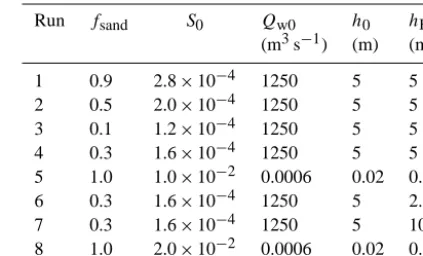
We show three model runs in Fig. 6 with the portion of sand in the upstream sediment discharge set to 25, 50, and 75 %. The resultant deltas differ systematically based on the input mud fraction in the following characteristics, which are consistent with those found in the investigation on the effects of sediment cohesion by Edmonds and Slingerland (2009).
– On a sandy delta the channels are relatively shallow and
mobile, without well-defined levees. Flow is less con-fined. There are large areas of sheet flow. The shoreline is smooth and the delta grows roughly in a semicircular shape.
Table 2.List of delta model runs and parameter values.
Run fsand S0 Qw0 h0 hB
(m3s−1) (m) (m)
1 0.9 2.8×10⁻⁴ 1250 5 5
2 0.5 2.0×10⁻⁴ 1250 5 5
3 0.1 1.2×10⁻⁴ 1250 5 5
4 0.3 1.6×10⁻⁴ 1250 5 5
5 1.0 1.0×10⁻² 0.0006 0.02 0.02
6 0.3 1.6×10⁻⁴ 1250 5 2.5
7 0.3 1.6×10⁻⁴ 1250 5 10
8 1.0 2.0×10⁻² 0.0006 0.02 0.02
– On a muddy delta, channels are deeper and stable, with
well-defined levees. Channels tend to elongate. The shoreline is rugose, and deltas build in different direc-tions by switching lobes.
– The contrast in the model-predicted roughness between
a sandy and muddy delta is illustrated in Fig. 7, where plots of the time variation of the ratio of number of cells on the shoreline to average delta radius (measured in number of cells) is presented. In these calculations, the shoreline is defined using the opening-angle method (OAM) developed by Shaw et al. (2008), employing an elevation threshold of−1 m and an opening-angle threshold of 30◦. Also note that the calculation of the roughness ratio in Fig. 7 is made across the range of time intervals where the predicted delta consists of sev-eral lobes but has not yet filled the calculation domain.
4.2 Experimental fan deltas
Laboratory experiments, numerical modeling and field obser-vation are three important approaches of understanding the formation of deltas. Because we would like to test our model across as wide a scale range as possible, we include experi-mental deltas at laboratory scales. To do this, we change the domain to a lattice grid of 90 by 180 cells with a cell size of 0.02 m. The inlet channel is still five-cells wide but has a flow depth of 0.02 m and a water discharge of 0.6 L s−1. Basin wa-ter depth is 0.02 m. The reference slope is set at 0.02. The time step is estimated at 1.67 s. Sediment input is considered to be coarse-grained only. These conditions are representa-tive of laboratory experiments such as those reported by Re-itz and Jerolmack (2012).
Figure 6.Time series of delta formation with different ratios of sand and mud flux (runs 1, 2 and 3). The time interval between rows is roughly 200 days of delta building time with continuous bank-full discharge.
Figure 7.Comparing shoreline roughness between simulated deltas with input sand fractions of 25, 50, and 75 %. Shoreline roughness here is measured by the ratio between (i) the number of cells in the domain that contain a piece of shoreline of the simulated delta, and (ii) the average radius of the delta toposet in number of cells.
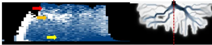
velocity greater than 50 % of the characteristic flow velocity) and plot it against time (Fig. 8g). Each avulsion event can be identified by a sudden drop of the wet fraction followed by a relatively slow rise caused by backfilling and flooding. An avulsion timescale estimated from this plot is in the range of 5–10 min, a value that is of the same order as the laboratory observations made by Reitz and Jerolmack (2012).
4.3 Effects of basin depth
Figure 8. The series of images matches the avulsion cycles observed in physical experiments (Reitz and Jerolmack, 2012): (a) channelizes, (b) pushes out the shoreline (only deposits at the channel mouth), (c) flares out locally to establish a semicircular lobe (deposits minilobes around original channel mouth by local avulsions and sheet flow), (d) backfills (channel widens), (e) floods, and (f) channelizes again. Note that the time interval between (d) and (e) is about 4 times longer than any other pair of consecutive frames.
to the description of Storms et al., while the deep basin delta has similar outcomes but the middle ground bar and avulsion over the levee are not as clear in the RCM results.
The differences between a shallow and deep receiving basin, according to our model results, are the following:
– Channels will still try to maintain the same unit power
of transporting sediment by maintaining a certain cross-sectional geometry with levees on the side and erosion or deposition on the bottom.
– In general, a distributary channel network shoals up and
channels are stable at shallower depths going seaward. With a shallow basin the amount of work is reduced. Also, the narrow space promotes the splitting of flow which enhances the growth of a distributary network.
– A deep basin increases the timescale of establishing a
stable channel and, therefore, introduces stronger
com-Figure 9.Two model runs (runs 6 and 7) with different basin depths and everything else the same. The shallow basin delta is dominated by more frequent bifurcations while the deep basin delta is domi-nated by few channels with more avulsions.
petition among channels by allowing larger differences to develop.
– The total number of active channels is higher in the
shal-low basin case, with about 5–6 channels, as compared to 1–3 channels in the deep-basin case.
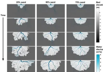
Finally, we note two interesting emergent features from our model that have also been observed in the field at Wax Lake Delta by Shaw (2013) and Shaw et al. (2013) (Fig. 10). First, the channels in the shallow basin delta are initially erosional, and carve into the basin bottom. This is consistent with the observations at the Wax Lake Delta (Shaw et al., 2013). Sec-ond, the channel network on this delta develops “tributary” subnetworks on islands (highlighted in Fig. 10), which col-lect flow both from tie channels directly connected to the main channel network and from sheet flow topping the levees into the islands. As to whether this subnetwork is erosional or depositional, Shaw (2013) points out that at least the chan-nels comprising it are likely not favorable for deposition. In our model results, we notice the following process that might explain the situation.
1. The subnetwork mainly collects fine sediment from the main channel network, which requires a much slower flow to settle.
2. As the tributary subnetwork joins into bigger trunk channels, the ability of the flow to carry sediment in-creases.
Figure 10.Flow features on the island of a delta formed in a shal-low basin. (a) Model result from run 6, where basin depth (2.5 m) is only half of the inlet channel depth (5 m); (b) Wax Lake Delta, where basin depth (<5 m) is much lower than the inlet channel depth (>20 m); (c) schematic drawing showing the “tributary” flow feature on the island (Shaw et al., 2013) observed both in the field (Shaw, 2013) and in our numerical model results.
deposited is very similar to a normal channel that has a coarser bar-like structure at the mouth.
5 Recording of stratigraphy
A delta writes (and rewrites) its own autobiography by build-ing a sedimentary record from deposition and erosion. These sedimentary records allow us understand the past and to use delta deposits to reconstruct their range of natural behavior. Therefore, the ability to record stratigraphy in a delta for-mation model enables us to directly investigate the connec-tion between surface and subsurface processes. In this model, we have two methods that track the stratigraphy of model-produced deltas: the first method tracks the distribution of coarse and fine sediment by recording the percentage of sand in each deposition event; and the second method tracks the age of the deposit by labeling each deposition event with the time that its sediment enters the domain from the inlet chan-nel.
To track stratigraphy each cell in the domain is viewed as a storage column (shown in Fig. 2), and the volume be-low the bed surface is further divided into thin layers of an equal thickness (these layers are visible especially in Figs. 11 and 12). The thickness is chosen to be about a thousandth of the reference depth, although it can be set to different val-ues to allow for different vertical resolutions. Each layer is recorded with a value associated with it – at present it is ei-ther the percentage of sand (a value between 0 and 1) or the age of the deposit (represented by the number of time step).
For example, if a cell has net deposition, the volume it re-ceived from passing parcels will fill up as many layers as needed above the previous bed surface, and all values associ-ated with these layers are set to the ratio between the volume of sand deposited and the total volume of sediment deposited during this time step. If a cell has net erosion, the bed sur-face will be lowered and all values associated with the layers above the new bed surface will be erased (by resetting these values to−1 in the code).
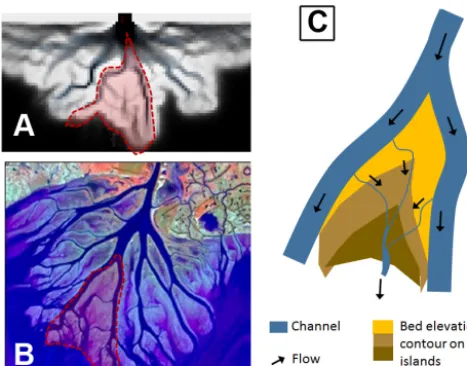
Here we present two examples. (1) We take a sample run of a field-scale delta and 30 % sediment input (run 4). In Fig. 11, we show a stratigraphic slice in the dip direction along the center line of the inlet channel. In Fig. 12, we show the time series of the stratigraphic slice in the strike direction about 20 cells (1 km in this case) away from the inlet channel. In both figures white represents pure sand and dark blue rep-resents pure mud, with mixed deposits represented by linear combinations of the two endmembers. Generally speaking, coarse sediment (sand) can be found in channel belts and mouth bars, while fine sediment (mud) can be found in distal regions such as the bottom set of the delta, on the floodplain or in abandoned channels. (2) In Fig. 13 we show a sample model run for laboratory conditions (run 8). Note the evolu-tion of the area pointed to by the yellow arrow. The series of images shows the deposition sequence from an individual avulsion event.
6 Discussion
Figure 11.Stratigraphy slice in the dip direction of run 4 (30 % sand input). Note the layering of coarse and fine grains over time. Yellow arrow points to the bottom layer that accumulates fine grains at the bottom set of the delta; orange arrow points to the coarse grain layer deposited by channels that used to be active at that location; the two together show the classic “coarsening-up” pattern in stratigraphy. The red arrow points to the fine grains deposited after the channels are abandoned.
Figure 12.Time series of the stratigraphic slice in the strike direction about 20 cells (1 km) away from the inlet channel. Note that be-tween (b), (c) and (d), in the yellow box, the abandoned channel belts are covered by muddy floodplain deposits. Also note that bebe-tween (e) and (f), in the light gray box, a mouth bar quickly deposits a significant amount of sand.
noncohesive sediment behaviors through a flow strength and flow velocity terms, respectively, was able to build both elon-gated bird-foot and multichannel fan deltas. Part 2 of this work further explores the hydrodynamic mechanism of the water surface and investigates the feedback between the flow solver and the sediment transport processes in determining channel bifurcations.
The need for accurate representation of some of the phys-ical details in DeltaRCM is quite striking compared to the success of even fairly radical reduced-complexity approaches in modeling other morphodynamic environments such as ero-sional landscapes (e.g., Willgoose et al., 1991), braided rivers (e.g., Murray and Paola, 1994) and eolian bedforms (e.g., Werner, 1995). So why is it that deltas seem to require more attention to detail? Can we learn anything from this
Figure 13.Time series of a delta produced by DeltaRCM with laboratory settings, and stratigraphy slices in the strike direction about 20 cells (0.4 m) away from channel inlet. Note the evolution of the area pointed to by the yellow arrow. (a) A concave shoreline – empty space in stratigraphy; (b) channel begins to receive water and sediment – deposition begins; (c) more water and sediment switch to the channel – space is filled-up quickly; (d) full avulsion completed – a channel is established by water eroding existing deposits; (e) backfilling causes flooding and the channel loses its advantage – the channel is refilled and there is a discontinuity in deposition age (yellowish green in the upper portion and bluish green in the lower portion).
deltas because deltas are low-gradient environments where the transport direction and capacity are to some extent de-coupled from bed elevation and slope. To be more specific, (1) bed slope in low-gradient environments is often uncor-related with flow direction and strength; for example, bed slope points opposite to the direction of flow where channels shoal up towards the shoreline; (2) the water surface, which dominates local flow routing, is largely independent of bed topography; (3) the typical Froude-number flow in low-gradient deltaic environments creates strong backwater ef-fects that imply strong nonlocality in flow and sediment flux control (Lamb et al., 2012; Nittrouer et al., 2011) – meaning that downstream conditions control upstream flow dynamics (Hoyal and Sheets, 2009); and (4) river mouth and shore pro-cesses such as waves and tides also control the overall mor-phology of deltas, providing additional process complexity.
According to Werner (1995), for a nonlinear and dissipa-tive system, considerable simplification can be applied if the system exhibits the following two properties: (1) it has a fi-nite number of steady states as “attractors”, and (2) it has macroscopic emergent behaviors that are self-organized and consistent with, but decoupled, from microscopic physics. If we compare drainage networks with deltas, the former ex-hibits a strong generic pattern and scale-invariant properties expressed in generalizations such as Horton’s laws (Horton, 1945). In contrast, the networks on deltas have many vari-eties, responding to a wide range of processes; no universal geometry applies to them all. Regarding model complexity, the lack of universality in the system pattern indicates the re-quirement for a more detailed, system-specific approach in modeling them.
So, is the low gradient the main cause of the modeling difficulty, making deltas more “unforgiving” than erosional landscapes in terms of the accuracy of hydrodynamic cal-culation? For cellular models that use explicit flow routing schemes, the complexity level rises as factors other than to-pographic slope alone determine water and sediment routing. It also increases with nonlocality in the broad sense of the sensitivity of dynamics at one point to conditions far away in the system. Other contributing factors such as water surface gradient and flow inertia weigh in as the overall topographic gradient decreases. For example, dune fields may have very low to zero average topographic slope, but they have lo-cally high steepness meaning that, as in erosional landscapes, the sediment dynamics are dominated by bed topography. In deltas, however, the controlling factor is the relatively sub-tle water surface topography, therefore simple descriptions relating sediment deposition and erosion to e.g., local eleva-tion and slope give realistic dune field dynamics but do not work in deltas.
Can we be more systematic about evaluating the amount of detail needed to model a geomorphodynamic system? This is an important fundamental question in morphodynamic mod-eling, and we do not pretend to resolve it here. But our
expe-rience with DeltaRCM suggests the following guidelines as a starting point.
– For gravity-driven systems, the overall gradient of the
landform is one important index in the sense that in high-gradient systems the gradient alone is enough to route the flow.
– A closely related indicator is the wetted area fraction in
the sense that a combination of low wetted fraction and high topographic gradient is the limit in which steepest-path methods (Passalacqua et al., 2010) are sufficient to determine the flow path, without the need for simulation of the flow details.
– Froude number (Fr): as Fr tends to unity, the backwater
length tends to zero (Cui and Parker, 1997), so the sim-plification of a local normal-flow assumption provides a satisfactory means of accounting for momentum bal-ance in the flow.
– For systematic behaviors on scales greater than the
backwater length scale, in-channel-scale hydrodynamic details can be resolved at much lower complexity; this applies for example to avulsion models that use single-cell-wide threads to represent channel belts (Jerolmack and Paola, 2007).
– Whether the system to be modeled exhibits a strong
generic pattern or scale-invariant (e.g., fractal) proper-ties, the lack of universal patterns in a dynamic system is an indicator of sensitivity to local detail.
We see the potential of this type of modeling as analogous to that of laboratory experiments, which can also provide useful insight despite not capturing all the details of complex natu-ral systems (Paola et al., 2009). The strength of RCMs is to serve as (1) exploratory models that allow for direct represen-tation of phenomenological observation; (2) a tool to iden-tify those aspects of large-scale system behavior that are not sensitive to the details of smaller-scale processes; and (3) a framework for hybrid modeling in which higher-resolution model results can be integrated where precise description of smaller-scale processes is needed even for larger-scale dy-namics.
7 Conclusions
on a set of rules that distinguish bedload and suspended load; (4) bed sediment columns record the composition of coarse and fine material in layers; (5) a topographic diffusion pro-cess takes into account cross-slope sediment transport and bank erosion. By varying input conditions such as the ratio of coarse and fine sediment, reference slope, and dimensions of the domain, the simulated deltas yield a range of different behaviors that compare well to higher-fidelity model results and observations of field and experiment deltas.
We find that the relatively simple cellular representation of water and sediment transport is able to replicate delta morphology at the scale of channel dynamics, including the emergent channel network with channel extension, bifurca-tion and avulsion. Here, we summarize the basic components needed for a RCM to produce major static and dynamic fea-tures of river deltas:
– a depth-averaged flow field that guides sediment
trans-port
– a nontrivial water surface profile that accounts for
back-water effects at least in the main channels
– representation of both bedload and suspended load – topographic steering of sediment transport.
Even at the RCM level of modeling, the following items still require a physically consistent treatment:
– the instability at channel mouths that creates bars and
subsequent bifurcation
– the variation in water surface profile associated with
lobe extension that causes channel avulsion
– water surface slope along channel sides which creates
Appendix A
Table A1.List of notations.
Symbol Definition and unit Symbol Definition and unit
α Topographic diffusion ns Number of sediment parcels
coefficient (m2s−1) (–)
γ Partitioning parameter for Pi Routing probability (–) routing by inertia and by free
surface (–)
1i Cellular distance (–) Qcell Total discharge at a cell (m3s−1)
δc Grid size (m) Qw0 Total water discharge from
inlet channel (m3s−1)
ε Diffusion coefficient for water Qs0 Total sediment discharge surface smoothing (–) from inlet channel (m3s−1)
η Bed/land elevation (m) Qp_water Discharge represented by a water parcel (m3s−1)
ηshore Threshold bed elevation for qs_cap Sediment flux capacity at a marking shoreline (m) cell (m2s−1)
θ Exponent of depth dependence qs_diff Diffusive sediment flux at a
(–) cell (m2s−1)
$ Underrelaxation coefficient for qs_loc Local coarse sediment flux at
water surface (–) a cell (m2s−1)
di Cellular unit direction (–) qw=(qx,qy) Water unit discharge vector (m2s−1)
F Routing direction (–) Ri Flow resistance (–)
Fint Routing direction by inertia (–) S0 Reference slope (–) Fsfc Routing direction by water 1t Time step (s)
surface (–)
fsand Fraction of sand (–) U0 Reference velocity (m s−1)
H Water surface elevation (m) Udep,Uero Threshold velocity for deposition and erosion (m s−1)
HSL Sea level (m) Uloc Local velocity at a cell (m s−1)
Hsmooth Smoothed water surface Ushore Threshold velocity for marking
elevation (m) shoreline (m s−1)
Htemp Temporary water surface u=(ux,uy) Flow velocity vector (m s−1) solution (m)
h Water depth (m) Vp_sed Initial volume of a sediment parcel (m3)
h0 Reference water depth (m) Vp_dep Volume removed from a sediment parcel by deposition (m3)
hB Basin water depth (m) Vp_ero Volume added to a sediment parcel by erosion (m3)
hdry Threshold water depth for dry Vp_res Remaining volume of a
land (m) sediment parcel (m3)
Nvisit Number of water-parcel visits at V0 Reference volume (m3) a cell (–)
Nx,Ny Number of cells in thexand 1Vs Total volume of sediment
ydirections of the input at each time step (m3) computational domain (–)
N0 Number of cells across inlet W Width of inlet channel (m) channel (–)
The Supplement related to this article is available online at doi:10.5194/-15-67-2015-supplement.
Acknowledgements. This work was supported by the National Science Foundation via the National Center for Earth-surface Dynamics (NCED) under agreement 0120914 and EAR-1246761. This work also received support from the National Science Foundation via grant FESD/EAR-1135427 and from ExxonMobil Upstream Research Company. The authors thank P. Passalacqua, D. A. Edmonds, N. Geleynse, and J. Martin for discussions and comments. The authors also thank S. Castelltort, R. Slingerland and A. Ashton for their insightful comments and reviews.
Edited by: S. Castelltort
References
Cui, Y. and Parker, G.: A quasi-normal simulation of aggradation and downstream fining with shock fitting, Int. J. Sediment Res., 12, 68–82, 1997.
Edmonds, D. A. and Slingerland, R. L.: Mechanics of river mouth bar formation: implications for the morphodynamics of delta distributary networks, J. Geophys. Res., 112, F02034, doi:10.1029/2006JF000574, 2007.
Edmonds, D. A. and Slingerland, R. L.: Significant effect of sedi-ment cohesion on delta morphology, Nat. Geosci., 3, 105–109, 2009.
Fagherazzi, S. and Overeem, I.: Models of deltaic and inner con-tinental shelf landform evolution, Annu. Rev. Earth Pl. Sc., 35, 685–715, 2007.
García, M. and Parker, G.: Entrainment of bed sediment into sus-pension, J. Hydraul. Eng., 117, 414–435, 1991.
García, M. H.: Sedimentation Engineering: Processes, Measure-ments, Modeling, and Practice, American Society of Civil En-gineers, Reston, VA, 1132 pp., 2008.
Galloway, W. E.: Process framework for describing the morpho-logic and stratigraphic evolution of deltaic depositional systems, in: Deltas, Models for Exploration, Houston Geological Society, Houston, TX, 87–98, 1975.
Geleynse, N., Storms, J. E. A., Stive, M. J. F., Jagers, H. R. A., and Walstra, D. J. R.: Modeling of a mixed-load fluvio-deltaic system, Geophys. Res. Lett., 37, L05402, doi:10.1029/2009GL042000, 2010.
Hajek, E. A. and Wolinsky, M. A.: Simplified process modeling of river avulsion and alluvial architecture: connecting models and field data, Sediment. Geol., 257–260, 1–30, 2012.
Heller, P. L., Paola, C., Hwang, I.-G., John, B., and Steel, R.: Ge-omorphology and sequence stratigraphy due to slow and rapid base-level changes in an experimental subsiding basin (xes 96-1), AAPG Bull., 85, 817–838, 2001.
Horton, R. E.: Erosional development of streams and their drainage basins, Geol. Soc. Am. Bull., 56, 275–370, 1945.
Hoyal, D. C. and Sheets, B. A.: Morphodynamic evolution of experimental cohesive deltas, J. Geophys. Res., 110, F02009, doi:10.1029/2007JF000882, 2009.
Jerolmack, D. J. and Paola, C.: Complexity in a cellular model of river avulsion, Geomorphology, 91, 259–270, 2007.
Kim, W., Mohrig, D., Twilley, R., Paola, C., and Parker, G.: Is it feasible to build new land in the Mississippi River Delta?, EOS Trans. Am. Geophys. Un., 90, 373–374, 2009.
Lamb, M. P., Nittrouer, J. A., Mohrig, D., and Shaw, J.: Backwater and river-plume controls on scour upstream of river mouths: im-plications for fluvio-deltaic morphodynamics, J. Geophys. Res., 117, F01002, doi:10.1029/2011JF002079, 2012.
Lesser, G. R., Roelvink, J. A., van Kester, J. A. T. M., and Stelling, G. S.: Development and validation of a three-dimensional mor-phological model, Coast. Eng., 51, 883–915, 2004.
Lorenzo-Trueba, J., Voller, V. R., and Paola, C.: A geometric model for the dynamics of a fluvially dominated deltaic system under base-level change, Comput. Geosci., 53, 39–47, 2013.
Meyer-Peter, E. and Müller, R.: Formulas for bed-load transport, in: Proceedings of the 2nd Meeting of IAHSR, Stockholm, Sweden, 39–64, 1948.
Murray, A. B.: Contrasting the goals, strategies, and predictions as-sociated with simplified numerical models and detailed simula-tions, Geophys. Monogr. Ser., 135, 151–165, 2003.
Murray, A. B. and Paola, C.: A cellular model of braided rivers, Nature, 371, 54–57, 1994.
Murray, A. B. and Paola, C.: Properties of a cellular braided-stream model, Earth Surf. Proc. Land., 22, 1001–1025, 1997.
Nittrouer, J. A., Mohrig, D., Allison, M. A., and Peyret, A. P. B.: The lowermost Mississippi River: a mixed bedrock-alluvial channel, Sedimentology, 58, 1914–1934, 2011.
Orton, G. J. and Reading, H. G.: Variability of deltaic processes in terms of sediment supply, with particular emphasis on grain size, Sedimentology, 40, 75–512, 1993.
Overeem, I., Syvitski, J. P. M., and Hutton, E. W. H.: Three-dimensional numerical modeling of deltas, in: River Deltas: Con-cepts, Models and Examples, edited by: Bhattacharya, J. P. and Giosan, L., SEPM Spec. Publ. 83, SEPM, Tulsa, OK, 13–30, 2005.
Paola, C.: Quantitative models of sedimentary basin filling, Sedi-mentology, 47, 121–178, 2000.
Paola, C. and Leeder, M.: Environmental dynamics: simplicity ver-sus complexity, Nature, 469, 38–39, 2011.
Paola, C., Straub, K., Mohrig, D., and Reinhardt, L.: The “unreason-able effectiveness” of stratigraphic and geomorphic experiments, Earth-Sci. Rev., 97, 1–43, 2009.
Paola, C., Twilley, R. R., Edmonds, D. A., Kim, W., Mohrig, D., Parker, G., Viparelli, E., and Voller, V. R.: Natural processes in delta restoration: application to the Mississippi Delta, Annu. Rev. Mar. Sci., 3, 67–91, 2011.
Parker, G., Muto, T., Akamatsu, Y., Dietrich, W. E., and Lauer, J.: Unravelling the conundrum of river response to rising sea-level from laboratory to field, Part I: Laboratory experiments, Sedi-mentology, 55, 1643–1655, 2008.
stud-ies in empirical geomorphic relationships, Water Resour. Res., 35, 3919–3929, 1999.
Seybold, H., Andrade Jr., J. S., and Herrmann, H. J.: Modeling river delta formation, P. Natl. Acad. Sci. USA, 104, 16804–16809, 2007.
Seybold, H. J., Molnar, P., Singer, H. M., Andrade, J. S., Herrmann, H. J., and Kinzelbach, W.: Simulation of birdfoot delta formation with application to the Mississippi Delta, J. Geophys. Res., 114, F03012, doi:10.1029/2009JF001248, 2009.
Seybold, H. J., Molnar, P., Akca, D., Doumi, M., Cavalcanti Tavares, M., Shinbrot, T., Andrade, J. S., Kinzelbach, W., and Herrmann, H. J.: Topography of inland deltas: observations, modeling, and experiments, Geophys. Res. Lett., 37, L08402, doi:10.1029/2009GL041605, 2010.
Shaw, J. B.: The kinematics of distributary channels on the Wax Lake Delta, coastal Louisiana, USA, PhD dissertation, Univer-sity of Texas at Austin, Austin, TX, 2013.
Shaw, J. B., Wolinsky, M. A., Paola, C., and Voller, V. R.: An image-based method for shoreline mapping on complex coasts, Geo-phys. Res. Lett., 35, L12405, doi:10.1029/2008GL033963, 2008. Shaw, J. B., Mohrig, D., and Whitman, S. K.: The morphology and evolution of channels on the Wax Lake Delta, Louisiana, USA, J. Geophys. Res.-Earth, 118, 1–23, 2013.
Storms, J. E. A., Stive, M. J. F., Roelvink, D. (J.) A., and Walstra, D. J.: Initial Morphologic and Stratigraphic Delta Evolution Re-lated to Buoyant River Plumes, Coastal Sediment’07, American Society of Civil Engineers, New Orleans, Louisiana, 736–748, 2007.
Sun, T., Paola, C., Parker, G., and Meakin, P.: Fluvial fan deltas: linking channel processes with large-scale morphodynamics, Water Resour. Res., 38, 26-1–26-10, 2002.
Syvitski, J. P. M., Kettner, A. J., Overeem, I., Hutton, E. W. H., Han-non, M. T., Brakenridge, G. R., Day, J., Vörösmarty, C., Saito, Y., Giosan, L., and Nicholls, R. J.: Sinking deltas due to human ac-tivities, Nat. Geosci., 2, 681–686, 2009.
Van Rijn, L. C.: Sediment transport II: Suspended load transport, J. Hydraul. Eng., 110, 1431–1456, 1984.
Werner, B. T.: Eolian dunes: computer simulations and attractor in-terpretation, Geology, 23, 1107–1110, 1995.