www.earth-surf-dynam.net/3/55/2015/ doi:10.5194/esurf-3-55-2015
© Author(s) 2015. CC Attribution 3.0 License.
Re-evaluating luminescence burial doses and bleaching
of fluvial deposits using Bayesian computational
statistics
A. C. Cunningham1,2, J. Wallinga3, N. Hobo3,4,5, A. J. Versendaal3, B. Makaske3,4, and H. Middelkoop5 1School of Geosciences, University of the Witwatersrand, Johannesburg, South Africa
2Centre for Archaeological Science, School of Earth and Environmental Sciences, University of Wollongong,
Wollongong, Australia
3Soil Geography and Landscape group & Netherlands Centre for Luminescence dating, Wageningen University,
Wageningen, the Netherlands
4Alterra, Wageningen University and Research Centre, Wageningen, the Netherlands 5Department of Physical Geography, Utrecht University, Utrecht, the Netherlands
Correspondence to: A. C. Cunningham ([email protected])
Received: 20 June 2014 – Published in Earth Surf. Dynam. Discuss.: 2 July 2014 Revised: 24 November 2014 – Accepted: 22 December 2014 – Published: 16 January 2015
Abstract. The optically stimulated luminescence (OSL) signal from fluvial sediment often contains a remnant from the previous deposition cycle, leading to a partially bleached equivalent-dose distribution. Although iden-tification of the burial dose is of primary concern, the degree of bleaching could potentially provide insights into sediment transport processes. However, comparison of bleaching between samples is complicated by sample-to-sample variation in aliquot size and luminescence sensitivity. Here we begin development of an age model to account for these effects. With measurement data from multi-grain aliquots, we use Bayesian computational statistics to estimate the burial dose and bleaching parameters of the single-grain dose distribution. We apply the model to 46 samples taken from fluvial sediment of Rhine branches in the Netherlands, and compare the results with environmental predictor variables (depositional environment, texture, sample depth, depth relative to mean water level, dose rate). Although obvious correlations with predictor variables are absent, there is some suggestion that the best-bleached samples are found close to the modern mean water level, and that the extent of bleaching has changed over the recent past. We hypothesise that sediment deposited near the transition of chan-nel to overbank deposits receives the most sunlight exposure, due to local reworking after deposition. However, nearly all samples are inferred to have at least some well-bleached grains, suggesting that bleaching also occurs during fluvial transport.
1 Introduction
The use of optically stimulated luminescence (OSL) for dat-ing Holocene fluvial deposits is widespread. However, flu-vial sediments are not ideal for OSL dating because the in-tensity of sunlight under water may not be sufficient to re-set the OSL signal in some grains prior to their deposition. The remnant OSL signal can then cause the burial dose to be overestimated, leading to an overestimate of the age. This
phenomenon is referred to as poor, partial or heterogeneous bleaching (e.g. Wallinga, 2002a).
pri-mary sediment source (Murari et al., 2007). For fluvial de-posits, poor bleaching might, for instance, reflect short trans-port distances or an old deposit acting as the primary source. To compare the bleaching between samples, it is first nec-essary to distinguish between the part of the equivalent dose (De) built up since the time of deposition and the poorly bleached remnant dose. Previous studies have avoided this issue by deliberately sampling modern or known-age sedi-ment. Such studies have indicated that bleaching is better in coarse sand-sized grains compared to finer grains (Olley et al., 1998; Truelsen and Wallinga, 2003), and may be depen-dent on depositional context (Murray et al., 1995; Schielein and Lomax, 2013) and transport distance (Stokes et al., 2001; Jain et al., 2004; and references therein).
Nevertheless, the inherent variability from sample to sam-ple makes definitive conclusions hard to come by. The main problem arises in distinguishing signal from noise: how much of the sample-to-sample variation in bleaching is due to physical processes, as opposed to random statistical fluc-tuations? Studies focusing on modern or known-age deposits seldom have enough samples for confident conclusions to be drawn, and no study has quantified the variation between ad-jacent samples. Moreover, the review of Jain et al. (2004) showed a discrepancy in residual doses of modern fluvial samples compared to young known-age samples, with mod-ern samples yielding larger residual doses. They argued that modern deposits may yet be remobilised, so their transport history is not representative of deposits preserved in the stratigraphic record.
Here we focus not on modern samples but on samples of various ages that have already been used for age estimation. This approach allows for more samples to be included, and avoids the bad-modern-analogue issue, but presents the addi-tional problem of separating out the burial dose from the rem-nant dose. For this purpose we have designed an age model specifically for these young, partially bleachedDe distribu-tions. We define the degree of bleaching by the proportion of grains that were well bleached upon deposition, rather than by the remnant dose. We apply the model to a suite of 46 samples from embanked floodplains of the lower Rhine in the Netherlands, and correlate the outcome with geomorphic data for each sample.
2 Methods
2.1 Samples and measurements
We use a data set of OSL measurements on a suite of 46 sam-ples from embanked floodplain deposits formed during the past 700 years. Different parts of the data set have been pre-sented by Hobo et al. (2010, 2014) and Wallinga et al. (2010). Samples come from four different sites, all located in the Rhine Delta in the Netherlands (Fig. 1). At each of the sites, several cores (diameter 14–19 cm) were taken in a cross sec-tion perpendicular to the river course (see Hobo et al., 2010,
Figure 1.Map showing the sample sites. The sites Brummen and Zwolle are along the river IJssel, whereas the other two sites (Neer-ijnen and OB1-3) are along the river Waal. Both are branches of the river Rhine. OB1-3 refers to two cores from the Hiensche Uiter-waarden and one core from the Gouverneursche polder.
for examples). Samples were extracted from the cores in sub-dued orange light and prepared using methods described by Wallinga et al. (2010). For each of the sample sites, cross sections were constructed based on the borehole database of Utrecht University (Berendsen and Stouthamer, 2002) and additional hand corings. The cross sections were interpreted to identify morphogenetic units (see also Hobo et al., 2014). For all samples, radionuclide concentrations were deter-mined with high-resolution gamma-ray spectroscopy, from which dose rates were estimated using standard conversion factors. Sand-sized quartz grains were extracted for single-aliquot regeneration OSL measurements (Murray and Win-tle, 2003) for equivalent-dose measurements. Details of the procedure are described by Hobo et al. (2010) and Wallinga et al. (2010). The grain-size fractions varied between samples (180–212 µm, 180–250 µm or 90–180 µm), due to differences in texture of the sampled deposit. The measurement proto-cols were similar for all samples. The dose response was de-fined using a single regenerative dose (Wallinga et al., 2010), net OSL signals were defined using the early background subtraction (Cunningham and Wallinga, 2010) and low pre-heat temperatures were selected to avoid thermal transfer (e.g. Truelsen and Wallinga, 2003).
distal overbank, overbank, proximal overbank, channel); the sediment texture (clay, loam, silt, sand, coarse sand/gravel); the dose rate; the De; and the OSL age (although De and OSL age are derived from the model, they can also be con-sidered as predictor variables; the dose rate may indirectly af-fect the bleaching statistic). Table S1 (Supplement) provides an overview of all variables that are considered.
2.2 Statistical rationale
We seek to define a poor-bleaching score based on the mea-sured De distribution, which can then be used to compare bleaching between samples. Previous attempts have applied a statistical model directly to theDedistribution to define a summary statistic (e.g. theF statistic; Spencer et al., 2003 – skewness and kurtosis applied to single-grain (SG) distri-butions; Bailey and Arnold, 2006). This type of approach may be valid if the observed De distribution is a function of the burial dose and remnant dose. For multi-grain (MG) aliquots, the OSL signal comes from many grains; theDefor an aliquot is the average of those grains, weighted by their OSL sensitivity (e.g. Wallinga, 2002b; Duller, 2008; Cun-ningham et al., 2011). Therefore, for MG data sets, theDe distribution is a function of the burial and remnant doses, and also the aliquot size and the single-grain OSL sensitivity distribution.
Aliquot size and SG sensitivity may vary between sam-ples, so for a statistic to be useful, it must be independent of these factors for the range of samples considered. A model defined directly on theDe distribution of young samples is also likely to be sensitive to the burial dose, as the measure-ment precision decreases with decreasing De. Our data set contains many samples, measured over several years on dif-ferent OSL readers. While the SG sensitivity distributions are likely to be similar (as all samples are from Rhine de-posits), the aliquot size varies both between and within sam-ples: measurements used either 2 or 3 mm mask size, with grain sizes of 180–212, 180–250 or 90–180 µm. A statistic defined from the MG aliquot De distribution (such as the burial dose, overdispersion, degree of bleaching) may not have any real-world meaning, because the data are affected by the confounding variables of aliquot size and SG sensi-tivity. The meaningful parameters operate at the single-grain level, so the approach we take here is to estimate what combi-nation of single-grain parameters would lead to the measured MG De distribution. There are two parts to the procedure. First, we define how the MGDedistribution is derived from single-grain parameters. Second, we use Bayesian compu-tational statistics to estimate the value each parameter must take to reproduce the observed MGDedistribution.
2.3 From single-grain parameters to the multi-grain-aliquot distribution
2.3.1 The single-grain sensitivity distribution
The magnitude of the OSL signal induced by a given radia-tion dose varies from grain to grain. The sensitivity distribu-tion also varies between samples (Duller et al., 2000). Quan-tifying the SG sensitivity is important for dating partially bleached samples, because it governs the extent of averag-ing across multi-grain aliquots (Cunnaverag-ingham et al., 2011). We therefore need to define the SG sensitivity distribution in order to simulate an MGDedistribution. While this can be done using a single-grain measurement system, there are practical difficulties: some grain holes may be empty and some may contain more than one grain, and with many sen-sitivity values clustered around zero, it is difficult to distin-guish signal from noise.
Here we use computational Bayesian statistics to estimate the SG sensitivity distribution from the MG sensitivity data. The first step is to parameterise the SG sensitivity, for which we use the gamma distribution. The gamma distribution can be formatted with two parameters: a shape parameteraand a scale parameterb. By altering these parameters, the gamma distribution can comfortably fit a range of measured SG sen-sitivity distributions (Fig. 2a). Moreover, when a MG aliquot is simulated from SG sensitivity data, the MG sensitivity distribution can also be fitted with a gamma distribution (Fig. 2b). For measured data, we already know the MG sen-sitivity distribution (from the regenerative-dose signal) and the approximate number of grains in the aliquot (from the grain size and mask size); we can therefore estimate the pa-rameters a andb of the SG sensitivity distribution using a computational Bayesian procedure similar to that described below.
2.3.2 Modelling theDedistribution The single-grain parameters are as follows:
a. SG sensitivity, drawn from the gamma distribution with parameters:
– adescribes the shape (i.e. skewness); – bdescribes the scale.
b. The burial dose, drawn from a normal distribution with parameters:
– γ: mean, in Gy;
– σbSG: relative standard deviation of the burial dose (fixed as 0.20 for this work).
c. The remnant dose, drawn from the positive part of a nor-mal distribution with mean of 0 and:
Figure 2.(a) Three SG sensitivity distributions presented by Duller
et al. (2000) from SG measurements (dotted lines). Each has been approximated using the gamma distribution, with sample name and shape parametera indicated. (b) Simple stochastic simulation of a multi-grain-aliquot sensitivity distribution. The simulation uses the measured SG sensitivity data set RBM2 (from Duller et al., 2000), with parametersng=200 andna=1000. The MG
sensitiv-ity distribution can also be fitted using the gamma distribution, with
a=5.70. The shape of the gamma distribution is indicated in the figure, with theyscale normalised to the peak of the histogram.
– p: proportion of well-bleached grains.
d. Additional parameters:
– ng: number of grains in each aliquot; – na: number of aliquots.
The simulated natural OSL signal from na aliquots is the sum of the signal fromnggrains, with Poisson noise added. Each grain is assigned a sensitivity value (per Gy) drawn from the gamma distribution with parameters a andb, and an indicative dose. The indicative dose combines the burial dose, drawn from a normal distribution, and a remnant dose, drawn from a half-normal distribution. The number of grains in each aliquot that have a remnant dose is drawn from the binomial distribution with parametersngand 1−p. TheDe
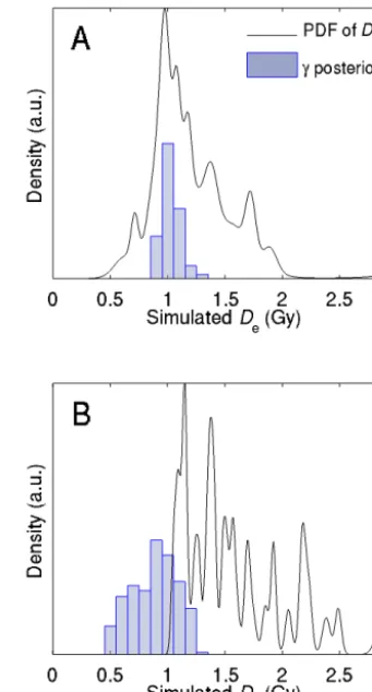
Figure 3.Posterior distribution of the burial doseγ for simulated data of aliquots of (a) 80 grains and (b) 300 grains. The “given” burial dose is 1 Gy; other parameters are specified in Table 1. The simulatedDedistributions are visualised with probability density
functions (PDFs).
is determined by constructing a dose-response curve in the same way as measured data, i.e. one regenerative point of 3 Gy, sensitivity-corrected (although no sensitivity change is added), and subject to the same rejection criteria. Where dif-ferent aliquot sizes are used in the measured data, these are replicated in the simulation. The number of grains per aliquot (ng) is approximated using the known mask size and grain size, assuming spherical grains and a 0.7 packing density (i.e. quartz grains cover 70 % of the mask surface).
2.4 Computational Bayesian solution
the posterior distribution, which requires intensive computa-tion.
In our model, the posterior is sampled using a Markov chain Monte Carlo (MCMC) process. Single-grain param-eters for four Markov chains are drawn from a starting dis-tribution, and these parameters are then corrected to better approximate the target posterior. The approximate distribu-tions are improved at each step using the Metropolis algo-rithm. When the simulation has run long enough, each step can be considered a random draw from the target distribution. The length of the sequence is determined by the convergence of the Markov chains; this is monitored by comparing the within-chain and between-chain variance, following the pro-cedure of Gelman et al. (2004). The first half of each Markov chain is discarded to ensure that the choice of starting values does not influence the result.
2.4.1 Priors
Five parameters are determined in the computational pro-cessing:γ,σ,p,a andb. Each of these is assigned a prior distribution, which represents our knowledge of these param-eters before any measurements are undertaken. The priors could in future be determined from previous measurement data or, in the case of γ, from the stratigraphic order of the samples. For a andb, the priors are given by the posteri-ors obtained from the SG sensitivity model. For γ we use a uniform-positive prior, as we have no information on the burial dose and do not want to restrict it. The situation is dif-ferent when it comes to p andσ. There is an unavoidable conflict when estimating these two parameters: as the resid-ual dose gets smaller, at some point theDevalues cannot be distinguished from well-bleached Devalues. This problem, not unique to our model, could erroneously assign a lowp to a well-bleached sample, or high p to a poorly bleached sample (if σ is very small). To prevent this error, we spec-ify arbitrary cut-offs in the priors: the lower limit for σ is 0.25 Gy, and for p it is 0.05. As such, any sample that is poorly bleached to a very small extent (σ <0.25 Gy) will be inferred to be well bleached (highp). Very few samples are affected by the low-cut priors. In future, it will be useful to find an objective value for the low cut-off, probably varying with measurement precision.
2.4.2 Density evaluation
Parameters with positive values (γ,σ,a,b) are estimated on the log scale;p must lie between 0 and 1, and is therefore estimated on the logit scale (logit p=log(p/(1−p); this transforms the unit interval to the real number line). The sim-ulated MGDedistribution is compared to the measured dis-tribution using the models of Galbraith et al. (1999) as sum-mary statistics. This provides four sumsum-mary statistics to com-pare with the measured data (three from the three-component minimum-age model (MAM3), and one from the central-age
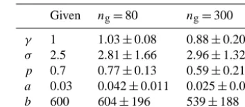
Table 1.Results of the simulation recovery: “recovered” values are defined by the mean and standard deviation of the posterior distri-bution.na=40.
Given ng=80 ng=300 γ 1 1.03±0.08 0.88±0.20
σ 2.5 2.81±1.66 2.96±1.32
p 0.7 0.77±0.13 0.59±0.21
a 0.03 0.042±0.011 0.025±0.008
b 600 604±196 539±188
model (CAM)). The likelihood term is defined by projecting these values onto the bootstrap likelihood distribution for the measured data (see Cunningham and Wallinga, 2012).
The model is run in two phases. The first is a short run, giv-ing an approximate range of the parameter space. The output of the first run is summarised by a multivariate normal dis-tribution, which is used to define the starting distribution and jumping distributions for phase two. The second phase is run until convergence.
2.5 Model validation
Here we perform a simulation-recovery test to check that the model is performing as expected. Single-grain parameters are chosen, and then used to simulateDe data for two different aliquot sizes (80 and 300 grains). Each data set is used as input for the model, and the SG parameters are then recon-structed. The results are given in Table 1, and plotted in Fig. 3 for the burial doseγ.
For both aliquot sizes, the SG parameters can be recon-structed (Table 1). Reconstruction of the 1 Gy burial dose is reasonably precise (8 %) for the 80-grain aliquots, and very close to the bootstrapped MAM3 estimate of the burial dose on the MG aliquot data set (1.03±0.08 Gy, usingσbof 0.16. σb is used in the MAM3 to allow for the expected disper-sion inDefrom well-bleached samples, and it changes with aliquot size). For the 300-grain aliquots, the estimate of the burial dose is imprecise but accurate, and lies mostly out-side the range of the MG aliquotDedistribution. For multi-grain aliquots, it is quite possible that none of the aliquots are indicating the burial dose, if at least one grain contribut-ing to the OSL signal on each aliquot is poorly bleached. The model is able to explore this possibility by making use of the MG sensitivity distribution and aliquots size. In con-trast, the bootstrap MAM3 applied to the MG data assumes some “well-bleached” aliquots exist, and therefore gives an overestimated burial dose of 1.15±0.03 Gy for this data set (σb=0.08).
A
NCL-1110008B
NCL-1107146C
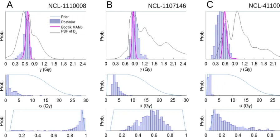
NCL-4110020Figure 4.Example model output for three samples that are (a) relatively well bleached, (b) moderately bleached and (c) poorly bleached. For each sample the posterior draws are indicated by the blue histograms, showing the burial doseγ(along with the bootstrap likelihoods of the MAM3 (bootlik MAM3) and a probability density function of theDedistribution), the residual doseσ, and the proportion of well-bleached
grainsp. Two sensitivity parameters,aandb, are also estimated in the model, but not shown here. All data sets are normalised to their maximum value.
distribution; it does not reconstruct the SG distribution itself. Testing the model against SG data for a real sample would not distinguish between the performance of the model and validity of the assumptions about SG parameters. The way around this would be to construct an artificial sample with a known dose distribution, like Roberts et al. (2000) and Sivia et al. (2004), but such an elaborate approach is outside the scope of this paper. Also, the mode of optical stimulation in single-grain measurement systems (green laser) differs from that used for MG aliquots for our study (blue LEDs). This prevents direct comparison between SG and MG, as com-ponent separation is wavelength-dependent (e.g. Singarayer and Bailey, 2003).
3 Results
The reconstructed SG sensitivity distribution is similar for all samples measured here, not surprising as they are all from recent Rhine deposits. The shape parameter a has a mean of 0.008 and standard deviation 0.003, indicating a highly skewed sensitivity distribution (more so than all of the ex-ample distributions in Fig. 2). The averaging effect on multi-grain aliquots is therefore very weak. The scale parameterb has a mean of 400 and standard deviation of 220. The es-timates of p are evenly spread between 0.2 and 0.95 (not shown). The uncertainty on p is typically large, except for those values close to 1.
The distribution ofσ is positively skewed; the mean is 2 Gy, and most values are below 8 Gy. However, high values of σ have very poor precision, coming from samples with highpin whichσ has little influence on theDedistribution. The susceptibility ofσ to outliers and topmakes it unsuit-able as an indicator of bleaching. The degree of bleaching is best defined byp, the proportion of well-bleached grains.
Three examples of the model output are shown in Fig. 4, each indicating a different degree of bleaching. For each sam-ple, the histograms indicate the posterior density of the burial doseγ and the two bleaching parametersσ andp. The two sensitivity parametersa andb are of lesser interest for this study, and are not shown. In Fig. 4a, the sample is inferred to be well bleached, and the burial-dose posterior is similar to the MAM3 bootstrap likelihood. This sample is affected by the problematic low-σ/high-p distinction alluded to earlier; the posteriorσis being influenced by the low-cut prior, caus-ing a low tail in the burial-dose posterior. Figure 4b shows a moderately bleached sample, with meanp=0.56. The pos-teriorσis well clear of the low-cut prior, and the burial dose is less precise but potentially more accurate than the MAM3 burial-dose estimate. A poorly bleached sample is shown in Fig. 4c (meanp=0.25, but affected by the prior). The burial-dose estimate is much less precise than the MAM3 estimate, but is permitted to be smaller than any of the measured MG De.
here). Such distributions are not well described by the mean and standard deviation, and thus may need to be summarised differently. We will not dwell on the issue here, but will leave it for future consideration.
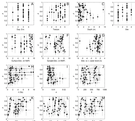
The mean (and standard deviation) of thepposterior pro-vides a useful summary statistic for between-sample com-parison. In Fig. 5,pis plotted against the potential geomor-phic variables (Fig. 5a–g), the other model-derived statis-tics (Fig. 5h–k), and finally the dose rate and model-derived age (Fig. 5l, m). A crude table of correlations is provided in the Supplement (Table S2), but is of limited use because it treats the ordinal variables of “depositional environment” and “texture” as if they are interval types. Nevertheless, there are some correlations among the predictor variables. For ex-ample, deeper samples are older and coarser (being channel deposits), and thus they have lower dose rates than the silty overbank samples. There are also significant correlations be-tween the sensitivity parametersaandband several predictor variables; these are probably due to inadequate aliquot-size estimates, as discussed in Sect. 4.
While there are no clear relationships betweenpand pre-dictor variables, some of the plots appear to indicate struc-ture beyond that expected through chance. Figure 5g shows that most of the best-bleached samples were located close to the modern mean water level. Figure 5k and m show a trend inp for the relatively young samples. In Fig. 6, the burial-dose estimate is compared directly to the original MAM3. The weighted mean ratio of γ to MAM3 minimum age is 0.97±0.025. Samples inferred to be relatively well bleached return very similar burial doses in both models, with com-parable precision. For poorly bleached samples, our model provides a smaller and less precise burial-dose estimate.
4 Discussion
4.1 Influences on bleaching
There appear to be significant relationships between the sen-sitivity parametersa andb, and several predictor variables: bothaandbare correlated with sample depth/elevation (Ta-ble S1). These relationships are difficult to explain in geo-morphic terms, but may be a manifestation of subtle differ-ences in grain size. Most measurements were carried out on grain-size range of 180–250 µm, with the aliquot sizeng es-timated from the grain size and mask size. This grain-size range still allows differences in the grain-size distribution of the natural sediment to be reflected on the disc. For fine sediments, the selected grain-size range will be at the upper tail of the grain-size distribution, resulting in a prepared frac-tion with many grains at the lower end of the sieved fracfrac-tion (i.e. 180 µm or just larger). In contrast, for coarse sediments the prepared fraction will be dominated by grains at the up-per end of the sieved fraction (i.e. 250 µm and somewhat smaller). The aliquots prepared from overbank sediment will therefore contain more grains than assumed in the model, and
aliquots prepared from channel sediments will contain fewer. These biases lead to an error in the model’s estimate of the SG sensitivity. The error would also feed through into the estimate of bleaching parameters. We should therefore ig-nore the correlations involving the sensitivity parameters for this data set, and be cautious about any relationship between bleaching parameters and depositional environment or depth, as both are correlated with sediment texture.
The large degree of uncertainty in our model results pre-vents convincing conclusions from being drawn. This uncer-tainty is again down to aliquot size. Firstly, the aliquot sizes used were often too large. Second, our post hoc estimates of the aliquot size were not sufficiently accurate (as noted by Heer et al., 2012). These issues affected model efficiency and outcome by amplifying the difficulty of distinguishing high pand lowσ. By contrast, recent measurements by Cunning-ham et al. (2015) included a grain-counting step, and allowed more emphatic conclusions to be drawn. Here, we do not feel confident in claiming either the existence or absence of geo-morphic controls on the basis of our results.
With these caveats established, it is worth considering two structures in the modelled data that might, possibly, have ge-omorphic significance. These concern the relationship be-tweenp and mean water level, and between p and model age, which are enlarged for clarity in Fig. 7. Figure 7a shows a cluster of relatively well-bleached samples coming from sediment deposited close to, or just above, the modern mean water level. This cluster might be telling something about the comparative strengths of bleaching during transport and deposition. The attenuation of light (especially UV/blue) un-derwater is well established (Berger, 1990), and if light in-tensity at deposition was the main control on bleaching, we might expect shallower sediments to be better bleached (Wallinga, 2002a). The clustering of highp values around the mean water level may therefore reflect a period of bleach-ing that occurs at deposition. However, close examination of the samples that are best bleached (NCL-111004, -5, -7, -8; NCL-2107157, -59, -61; NCL-4110018) shows that some of these are sandy channel deposits, whereas others are sand beds within silty overbank deposits, or silty overbank de-posits with sand admixtures. All these samples are indeed within a metre from the transition of channel to overbank de-posits. For the samples classified as channel deposits, depo-sition likely occurred on top of point bars, potentially with swash backwash operating and sub-aerial exposure likely (analogous to coastal beaches, which produce well-bleached quartz; e.g. Ballarini et al., 2003). For the well-bleached sam-ples from overbank deposits, we hypothesise that sand grains may have experienced aeolian reworking prior to final de-position and burial. Such aeolian reworking of sandy flood deposits has been documented following sand deposition on overbanks during high-discharge events of the Waal and Lek (Isarin et al., 1995; illustrated in Fig. 8).
best-A
B
C
D
E
F
G
H
I
J
K
L
M
Figure 5.The bleaching statisticp(proportion of grains well bleached) plotted against possible predictor variables (a–g), and other model-derived statistics and the dose rate (h–m). (a) Depositional environment on a scale of distal overbank (1) to channel (4). (b) Sediment texture is classed from clay (1) to coarse sand (5). Site classification in (d) is nominal. NAP is Dutch ordnance datum (≈mean sea level in Amsterdam). For classification details see Table S1.
bleached deposits, are obtained for samples with model ages around ∼0.10 ka. The youngest samples appear to be less well bleached (i.e. lowp), andpvaries a lot for the samples older than ∼0.10 ka. The same trends are observed when burial dose (Fig. 6k) or MAM3 age (not shown) is used in-stead of modelled age.
There are three possible reasons for the structure. It could be an artefact of the model through the high-p/low-σ prob-lem, but examination of the model output for these ples does not confirm this. Alternatively, it might be a sam-pling effect caused by coring from the floodplain down to-wards the high-p cluster at mean water level, but most of the high-psamples are older. A more intriguing explanation involves changes in river management over the last few
sed-0 0.25 0.5 0.75 1 1.25 0
0.2 0.4 0.6 0.8 1 1.2
MAM3 Minimum dose (Gy)
Modelled burial dose
γ
(Gy)
Figure 6.Comparison of burial-dose estimates. The modelled dose is defined by the mean and standard deviation of the posterior, and is compared to the original MAM3 minimum dose (usingσbof 12 %;
Galbraith et al., 1999). Squares indicate where the unlogged MAM3 was used (Arnold et al., 2009). The best-bleached samples are filled black (p >0.8), and the worst-bleached samples in red (p <0.3).
−4 −3 −2 −1 0 1 2 3 0
0.2 0.4 0.6 0.8 1
Elevation w.r.t mean water (m)
p
0 0.1 0.2 0.3 0.4 0.5 0.6 0
0.2 0.4 0.6 0.8 1
Age (ka)
p
(a)
(b)
Figure 7. Two possible structures in the proportion of well-bleached grainspversus predictor variables of Fig. 5, enlarged here for clarity. (a) Plotted against the sample elevation with respect to mean water level at each sampling site. A cluster of well-bleached samples appears at about the (modern) mean water level. (b) Plotted against model-derived age, showing a trend for the youngest sam-ples (age<0.10 ka). The onset of groyne construction is indicated at 0.15 ka.
Figure 8.A sand bar deposited close to the river Waal during high discharge (photo by Gilbert Maas, Alterra). Due to the absence of vegetation, such deposits may be reworked through aeolian pro-cesses, which may enhance bleaching for deposits formed above the mean water level.
iments. Secondly, sand bars within the channel disappeared, perhaps reducing light exposure of channel deposits during low flow. Thirdly, the groynes caused deepening of the chan-nel through bottom scour, enhancing the reworking of the underlying, high-residual-dose Pleistocene deposits.
4.2 Modelling the burial dose
The requirements of this project led us to develop a spe-cific “age model” for partially bleached, multi-grain-aliquot data. It uses Bayesian computational methods to estimate the parameters of the single-grain dose distribution, without the need for any single-grain measurements. Along the way, the parameters of the single-grain sensitivity distribution are estimated from multi-grain aliquot sensitivity data. Our ap-proach has significant advantages over existing models:
– The interaction of aliquot size and SG sensitivity is in-corporated, meaning that prior quantification of the av-eraging effect is not necessary.
– It includes uncertainty deriving from the number of aliquots consistent with the burial dose.
– It should provide an unbiased estimate of the burial dose, even when no aliquots are “well bleached”. Poorly bleached samples give a very imprecise, but still accu-rate, estimate of the burial dose.
– The degree of bleaching is quantified, and is potentially independent of the SG sensitivity, aliquot size and burial dose.
Of course, the validity of the outcome rests on a number of assumptions. The parameterisation of the SG dose and sensitivity distributions must be appropriate and, crucially, the estimate of aliquot size should be reasonable. This paper uses archive data, so aliquot size was estimated only roughly. When applied in future, careful grain counting should take place; this could be performed manually, or with a digital camera plus image-recognition software.
Compared to familiar and well-used age models in OSL dating (e.g. CAM and MAM3), this model is a different beast altogether. It requires more data to be input per sample, and careful consideration and specification of model parameters and priors. It includes the MAM3 (Galbraith et al., 1999) and bootstrap likelihoods (Cunningham and Wallinga, 2012) as a small part of it, and requires∼1 h of computer time to run per sample, provided no errors arise. We provide the code in the Supplement in order to spur further development in this field; we do not present a refined model for general applica-tion.
The model could be immediately improved by treating σbSG as an unknown parameter. At present, the model as-sumes that scatter in the single-grain burial-dose population is exactly 20 %. If it becomes possible to create a sample-specific estimate of σbSG (e.g. through radiation transport modelling; Cunningham et al., 2012; Guerin et al., 2012), it could be incorporated as a prior. The posterior σbSG would then be estimated along with γ, σ and p. A further step would be to incorporate stratigraphic information on sample order and/or age (e.g. Rhodes et al., 2003; Cunningham and Wallinga, 2012), although this would significantly increase computational time.
5 Conclusions
There are a particular set of challenges in estimating the de-gree of bleaching for unknown-age OSL samples, and these problems relate closely to the burial-dose calculation. We have begun to refashion the burial-dose calculation by using Bayesian computational statistics to reduce theDe distribu-tion into meaningful statistics. There are many novel aspects to our approach, such as parameterising the OSL sensitivity distribution and inferring single-grain statistics from small-aliquot measurements. We found that a good small-aliquot-size es-timate is particularly important for the model, and that our poor knowledge of aliquot size hampered our application of the model to archive data.
Nevertheless, the results do show some interesting fea-tures that may point to geomorphic controls on sediment bleaching. We found a concentration of well-bleached sam-ples around the modern mean water level, indicating to us that sediment receives a “kick” of bleaching upon deposition, through local reworking, in addition to the bleaching that oc-curs during transport. We also speculate on whether changes in the degree of bleaching over time could relate to river
man-agement changes, especially the construction of groynes in the lower Rhine around AD 1850.
Despite the limitations of this study, it seems clear that processes of sediment provenance, transport and deposition can influence the measured OSL signal. The challenge lies in extracting meaningful information from the OSL data. The computational approach explored in this study has real po-tential, and we hope aspects of our model will be taken for-ward.
The Supplement related to this article is available online at doi:10.5194/-15-55-2015-supplement.
Acknowledgements. This work was partially funded through a Technology Foundation (STW) VIDI grant (DSF.7553). We would like to thank Geoff Duller (Aberystwyth University) for making the data set on single-grain sensitivity distributions available. Zhixiong Shen and an anonymous reviewer are kindly thanked for their constructive comments. Matlab code is available in the supplement files.
Edited by: A. Lang
References
Arnold, L. J., Roberts, R. G., Galbraith, R. F., and DeLong, S. B.: A revised burial dose estimation procedure for optical dating of youngand modern-age sediments, Quatern. Geochronol., 4, 306– 325, doi:10.1016/j.quageo.2009.02.017, 2009.
Bailey, R. M. and Arnold, L. J.: Statistical modelling of single grain quartz De distributions and an assessment of procedures for esti-mating burial dose, Quaternary Sci. Rev., 25, 2475–2502, 2006. Ballarini, M., Wallinga, J., Murray, A. S., Van Heteren, S., Oost, A.
P., Bos, A. J. J., and Van Eijk, C. W. E.: Optical dating of young coastal dunes on a decadal time scale, Quaternary Sci. Rev., 22, 1011–1017, 2003.
Berendsen, H. J. A. and Stouthamer, E.: Palaeogeographic develop-ment of the Rhine-Meuse delta, The Netherlands, Van Gorcum, Assen, p. 268, 2002
Berger, G. W.: Effectiveness of natural zeroing of the thermolumi-nescence in sediments, J. Geophys. Res.-Solid Ea., 95, 12375– 12397, 1990.
Cunningham, A. C. and Wallinga, J.: Selection of integration time-intervals for quartz OSL decay curves, Quaterna. Geochronol., 5, 657–666, 2010.
Cunningham, A. C. and Wallinga, J.: Realizing the potential of fluvial archives using robust OSL chronologies, Quatern. Geochronol., 12, 98–106, 2012.
Cunningham, A. C., Wallinga, J., and Minderhoud, P. S. J.: Expecta-tions of scatter in equivalent-dose distribuExpecta-tions when using multi-grain aliquots for OSL dating, Geochronometria, 38, 424–431, 2011.
Cunningham, A. C., Evans, M., and Knight, J.: Quantifying bleach-ing for zero-age fluvial sediment: a Bayesian approach, Radiat. Measure., in press, 2015.
Duller, G. A. T.: Single-grain optical dating of Quaternary sedi-ments: why aliquot size matters in luminescence dating, Boreas, 37, 589–612, 2008.
Duller, G. A. T., Botter-Jensen, L., and Murray, A. S.: Optical dat-ing of sdat-ingle sand-sized grains of quartz: sources of variability, Radiat. Measure., 32, 453–457, 2000.
Galbraith, R. F.: On plotting OSL equivalent doses, Ancient TL, 28, 1–10, 2010.
Galbraith, R. F., Roberts, R. G., Laslett, G. M., Yoshida, H., and Ol-ley, J. M.: Optical dating of single and multiple grains of quartz from Jinmium rock shelter, northern Australia: Part I. Experi-mental design and statistical models, Archaeometry, 41, 339– 364, 1999.
Gelman, A., Carlin, J. B., Stern, H. S., and Rubin, D. B.: Bayesian data analysis, Chapman & Hall/CRC, Boca Raton, Florida, 2004. Guerin, G., Mercier, N., Nathan, R., Adamiec, G., and Lefrais, Y.: On the use of the infinite matrix assumption and associated con-cepts: A critical review, Radiat. Measure., 47, 778–785, 2012. Heer, A. J., Adamiec, G., and Moska, P.: How many grains are there
on a single aliquot?, Ancient TL, 30, 9–16, 2012.
Hesselink, A. W.: History makes a river: Morphological changes and human interference in the river Rhine, the Netherlands, Neth. Geogr. Stud., 292, 177, 2002.
Hobo, N., Makaske, B., Middelkoop, H., and Wallinga, J.: Re-construction of floodplain sedimentation rates: a combination of methods to optimize estimates, Earth Surf. Proc. Land., 35, 1499–1515, 2010.
Hobo, N., Makaske, B., Middelkoop, H., and Wallinga, J.: Recon-struction of eroded and deposited sediment volumes of the em-banked river Waal, the Netherlands, for the period AD 1631– present, Earth Surf. Proc. Land., 39, 1301–1318, 2014.
Isarin, R. F. B., Berendsen, H. J. A., and Schoor, M. M.: De morfo-dynamiek van de rivierduinen langs de Waal en de Lek, in: Pub-lications and reports of the project ’Ecological Rehabilitation of the Rivers Rhine and Meuse’, RIZA report 49, RIZA – Rijksinsti-tuut voor Integraal Zoetwaterbeheer en Afvalwaterbehandeling, Lelystad, 1995.
Jain, M., Murray, A. S., and Botter-Jensen, L.: Optically stimulated luminescence dating: how significant is incomplete light expo-sure in fluvial environments?, Quaternaire, 15, 143–157, 2004. Middelkoop, H.: Embanked floodplains in the Netherlands;
Geo-morphological evolution over various time scales, Netherlands Geographical Studies 224, Boca Raton, Florida, p. 341, 1997. Murari, M. K., Achyuthan, H., and Singhvi, A. K.: Luminescence
studies on the sediments laid down by the December 2004 tsunami event: Prospects for the dating of palaeo tsunamis and for the estimation of sediment fluxes, Current Sci., 92, 367–371, 2007.
Murray, A. S. and Wintle, A. G.: The single aliquot regenerative dose protocol: potential for improvements in reliability, Radiat. Measure., 37, 377–381, 2003.
Murray, A. S., Olley, J. M., and Caitcheon, G. G.: Measurement of equivalent doses in quartz from contemporary water-lain sed-iments using optically stimulated luminescence, Quaternary Sci. Rev., 14, 365–371, 1995.
Olley, J., Caitcheon, G., and Murray, A.: The distribution of ap-parent dose as determined by optically stimulated luminescence in small aliquots of fluvial quartz: implications for dating young sediments, Quaternary Sci. Rev., 17, 1033–1040, 1998. Reimann, T., Notenboom, P. D., De Schipper, M. A., and
Wallinga, J.: Testing for sufficient signal resetting dur-ing sediment transport usdur-ing a polymineral multiple-signal luminescence approach, Quatern. Geochronol., 25, 26–36., doi:10.1016/j.quageo.2014.09.002, 2015.
Rhodes, E. J., Bronk Ramsey, C., Outram, Z., Batt, C., Willis, L., Dockrill, S., and Bond, J.: Bayesian methods applied to the in-terpretation of multiple OSL dates: high precision sediment ages from Old Scatness Broch excavations, Shetland Isles, Quaternary Sci. Rev., 22, 1231–1244, doi:10.1016/S0277-3791(03)00046-5, 2003
Roberts, R. G., Galbraith, R. F., Yoshida, H., Laslett, G. M., and Ol-ley, J. M.: Distinguishing dose populations in sediment mixtures: a test of single-grain optical dating procedures using mixtures of laboratory-dosed quartz, Radiat. Measure., 32, 459–465, 2000. Schielein, P. and Lomax, J.: The effect of fluvial environments on
sediment bleaching and Holocene luminescence ages – A case study from the German Alpine Foreland, Geochronometria, 40, 283–293, doi:10.2478/s13386-013-0120-y, 2013.
Singarayer, J. S. and Bailey, R. M.: Further investigations of the quartz optically stimulated luminescence components using linear modulation, Radiat. Measure., 37, 451–458, doi:10.1016/S1350-4487(03)00062-3, 2003.
Sivia, D. S., Burbidge, C., Roberts, R. G., and Bailey, R. M.: A Bayesian approach to the evaluation of equivalent doses in sed-iment mixtures for luminescence dating, Am. Inst. Phys. Conf. Proc., 735, 305–311, 2004.
Spencer, J., Sanderson, D. C. W., Deckers, K., and Sommerville, A. A.: Assessing mixed dose distributions in young sediments identified using small aliquots and a simple two-step SAR pro-cedure: the F-statistic as a diagnostic tool, Radiat. Measure., 37, 425–431, 2003.
Stokes, S., Bray, H. E., and Blum, M. D.: Optical resetting in large drainage basins: tests of zeroing assumptions using single-aliquot procedures, Quaternary Sci. Rev., 20, 879–885, 2001. Truelsen, J. L. and Wallinga, J.: Zeroing of the OSL signal as a
func-tion of grain size: investigating bleaching and thermal transfer for a young fluvial sample, Geochronometria, 22, 1–8, 2003. Wallinga, J.: Optically stimulated luminescence dating of fluvial
de-posits: a review, Boreas, 31, 303–322, 2002a.
Wallinga, J.: Detection of OSL age overestimation using single-aliquot techniques, Geochronometria, 21, 17–26, 2002b. Wallinga, J., Hobo, N., Cunningham, A. C., Versendaal, A. J.,