www.earth-syst-dynam.net/7/697/2016/ doi:10.5194/esd-7-697-2016
© Author(s) 2016. CC Attribution 3.0 License.
Why CO
2
cools the middle atmosphere – a consolidating
model perspective
Helge F. Goessling1and Sebastian Bathiany2
1Alfred Wegener Institute, Helmholtz Centre for Polar and Marine Research, Bremerhaven, Germany 2Wageningen University, Wageningen, Netherlands
Correspondence to:Helge F. Goessling ([email protected])
Received: 11 March 2016 – Published in Earth Syst. Dynam. Discuss.: 18 March 2016 Revised: 27 July 2016 – Accepted: 8 August 2016 – Published: 29 August 2016
Abstract. Complex models of the atmosphere show that increased carbon dioxide (CO2) concentrations, while warming the surface and troposphere, lead to lower temperatures in the stratosphere and mesosphere. This cool-ing, which is often referred to as “stratospheric cooling”, is evident also in observations and considered to be one of the fingerprints of anthropogenic global warming. Although the responsible mechanisms have been iden-tified, they have mostly been discussed heuristically, incompletely, or in combination with other effects such as ozone depletion, leaving the subject prone to misconceptions. Here we use a one-dimensional window-grey radiation model of the atmosphere to illustrate the physical essence of the mechanisms by which CO2cools the stratosphere and mesosphere: (i) theblocking effect, associated with a cooling due to the fact that CO2absorbs radiation at wavelengths where the atmosphere is already relatively opaque, and (ii) the indirect solar effect, associated with a cooling in places where an additional (solar) heating term is present (which on Earth is partic-ularly the case in the upper parts of the ozone layer). By contrast, in the grey model without solar heating within the atmosphere, the cooling aloft is only a transient blocking phenomenon that is completely compensated as the surface attains its warmer equilibrium. Moreover, we quantify the relative contribution of these effects by sim-ulating the response to an abrupt increase in CO2(and chlorofluorocarbon) concentrations with an atmospheric general circulation model. We find that the two permanent effects contribute roughly equally to the CO2-induced cooling, with the indirect solar effect dominating around the stratopause and the blocking effect dominating otherwise.
1 Introduction
The laws of radiative transfer in the Earth’s atmosphere are a key to understanding our changing climate. With the ab-sorption spectra of greenhouse gases as one central starting point, climate models of increasing complexity have been built during the last decades. These models show that in-creased carbon dioxide (CO2) concentrations, while warm-ing the surface and the troposphere, lead to lower temper-atures in the middle atmosphere (MA; the stratosphere and the mesosphere) (Manabe and Strickler, 1964; Manabe and Wetherald, 1967, 1975; Fels et al., 1980; Gillett et al., 2003). Meanwhile, observations show a cooling trend in the MA during the satellite era until the most recent years; the neg-ative trend is especially large in the upper stratosphere and
in the mesosphere, although uncertainties also increase with height (Beig et al., 2003; Randel et al., 2009; Liu and Weng, 2009; Beig, 2011; Seidel et al., 2011; Thompson et al., 2012; Huang et al., 2014).
dis-cussed. The increase of CO2concentration contributed to the decrease of lower stratospheric temperatures, but only to a small extent (Shine et al., 2003). In the middle and upper stratosphere (and beyond), the CO2 increase has probably been the most important reason for the temperature decrease (Ramaswamy et al., 2001; Ramaswamy and Schwarzkopf, 2002; Shine et al., 2003; Thompson and Solomon, 2005). As ozone concentrations are expected to recover in the future, it seems likely that CO2-concentration trends will be of grow-ing importance also in the lower stratosphere (Stolarski et al., 2010; Ferraro et al., 2015).
The isolated effect of CO2on temperatures in the MA is rarely explained. Probably the most frequent argument found in textbooks (e.g., Pierrehumbert, 2010; Neelin, 2011) is re-lated to the ozone layer where a considerable part of the locally absorbed radiation is short-wave (solar) radiation. Therefore, the temperature around the stratopause exceeds the corresponding temperature in a hypothetical grey atmo-sphere by far. Because the main absorption bands of CO2are in the long-wave (LW) part and not in the solar part of the spectrum, an increase in CO2leads to increased emission of LW radiation while the rate of solar heating remains unal-tered. The excess of emission compared to absorption leads to a cooling. It should be stressed that the argument is related not to the depletion but to the mere presence of ozone (Ra-maswamy and Schwarzkopf, 2002). Although this effect is a major contributor to CO2-induced MA cooling (as we con-firm below), this explanation is less convincing in the mid-dle and upper mesosphere where there is unabated (observed and simulated) cooling despite the solar heating becoming weaker with height. Neither can this effect explain an im-portant difference between CO2and other long-lived green-house gases: while methane and nitrous oxide have a much weaker effect on MA temperatures compared to CO2, chlo-rofluorocarbons (CFCs) even tend to warm the lower strato-sphere (neglecting ozone depletion) (Dickinson et al., 1978; Forster and Joshi, 2005).
More complete explanations discern not only between so-lar and LW radiation, but treat the LW absorption spectra of greenhouse gases in more detail. Ramaswamy et al. (2001) and Seidel et al. (2011) point out that the balance of LW emission and LW absorption must be considered: any green-house gas emits simply according to its local temperature, but absorbs radiation emitted from certain distances (repre-sented by radiation mean free paths) depending on the ab-sorption spectrum of the gas and the atmospheric composi-tion. At the absorption bands of certain CFCs, the radiation mean free path of the atmosphere is large because the bands are located in the spectral window region. These CFCs thus absorb mainly radiation emitted from the warm surface and lower troposphere, but emit with the low temperatures of the MA. Consequently, increased CFC concentrations impose an LW warming tendency. Ramaswamy et al. (2001) point out that, in contrast, the radiation mean free path in the 15 µm band of CO2is small, implying that the radiation absorbed
by CO2in the MA mainly comes from the cold tropopause region.
Forster et al. (1997b) and Ramaswamy et al. (2001) ad-dress yet another aspect: the MA responds much faster than the rather inert surface-troposphere system. Hence, when greenhouse gases are added to the atmosphere, initially the MA cools because the radiation mean free path of the atmo-sphere has been reduced and the radiation arriving in the MA now stems from higher, colder levels of the troposphere. Af-ter this first phase of MA temperature adjustment, the surface and troposphere gradually warm, leading to increased up-ward LW radiation at the tropopause which warms the lower stratosphere.
All these effects, though mentioned in the literature and included in complex climate models, are rarely discussed to-gether. Furthermore, they are usually explained only heuristi-cally and not formalized with a conceptual model. The most popular educational model of the greenhouse effect, a global-mean grey atmosphere model with one ground level and a one-layer atmosphere (e.g., Neelin, 2011; Liou, 2002), can not explain CO2-induced MA cooling. Although Thomas and Stamnes (1999) introduce an atmospheric window to their conceptual model, they do not apply it to explain MA cool-ing. The same is true for more complex conceptual models (e.g., Pollack, 1969a, b; Sagan, 1969; Pujol and North, 2002), which are also not limited to the ingredients needed to ex-plain how CO2cools the MA.
parame-ters of the window-grey model in Appendix C. Appendix D provides technical details on Fig. 1.
2 The grey-atmosphere model
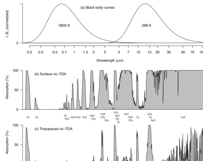
In the following we derive the vertical temperature profile of a grey atmosphere, first with only the atmosphere in thermal equilibrium and then assuming equilibrium also for the sur-face. We consider a vertically continuous grey atmosphere with horizontally homogeneous (global-mean) conditions. The grey atmosphere is transparent for solar radiation and uniformly opaque for LW radiation. Splitting the electromag-netic spectrum into a transparent solar band and an opaque LW band is a common approximation that is naturally sug-gested by (i) the well separated emission spectra of the Sun and the Earth (Fig. 1a) and (ii) the shape of the absorp-tion spectrum of the Earth’s atmosphere (Fig. 1b). The grey model accounts only for radiation while other processes of energy transfer (most importantly convection) are neglected. Greenhouse gases are assumed to be well-mixed and any ef-fects from clouds or aerosols are neglected. Assuming hor-izontally homogeneous conditions and the absence of scat-tering we apply the two-stream approximation (Liou, 2002; Pierrehumbert, 2010), meaning that we distinguish only up-ward and downup-ward propagating radiation (indicated by ar-rows in the subsequent equations). This leads to the differen-tial form of the radiative transfer equation (e.g., Goody and Yung, 1989; Pierrehumbert, 2010):
dL↑(z) dz =
1
µ
J−L↑(z)ρ(z)k, (1)
with radianceL, source termJ, geometric heightz, air den-sity ρ, mass absorption coefficient k, and µ=cos(θ) with the effective angle of propagationθ. To remove any angular dependence from the equations, we use the common assump-tion of an effective angle of propagaassump-tion of 60◦relative to the vertical, i.e., µ=1/2 (see Pierrehumbert, 2010, chap. 4.2). As we neglect scattering, J only consists of the long-wave blackbody emission, which is isotropic. Integrating Eq. (1) over the half sphere then yields
dF↑(z) dz =
σ T(z)4−F↑(z)ρ(z)k (2)
with irradianceF(in W m−2) and the Stefan-Boltzmann con-stantσ. Using the relative pressure deficit
h=1−p/psrf (3)
as vertical coordinate, wherepis pressure andpsrfis surface pressure, the radiative transfer equation reads
dF↑(h) dh =
σ T(h)4−F↑(h)
α . (4)
The absorption coefficientαis the only parameter of the grey model and describes the atmospheric opacity in the LW
band. Due to our definition of the vertical coordinateh,αis independent of h (in fact, it follows from hydrostatic bal-ance that α=k psrf/g). Also, h is proportional to optical thickness:τ=α h. Although we distinguish the parameter
αfrom the vertical coordinateh, our model is equivalent to similar approaches in popular textbooks of radiative trans-fer which usually choose optical depth (τ, also called optical thickness) as their vertical coordinate. For example, the op-tical thickness between a heighthand the top of the atmo-sphere, in our caseα(1−h), is identical toτ∞−τ in
Pierre-humbert (2010), toτ in Salby (1992), and toτ/µin Thomas and Stamnes (1999). In the latter two cases, the vertical axis points downwards, hence the reversed sign. In Thomas and Stamnes (1999), a parameterµstill appears in the equations as no assumption on the average direction of propagation is made.
Equation (4) is the spectrally integrated grey-absorption-case of Schwarzschild’s equation and holds analogously for downwelling LW radiation F↓. In radiative equilibrium F
must be free of divergence because other source or sink terms of heat are neglected. WithFtoa↓ =0,F↓is hence determined by
F↑(h)−F↓(h)=Ftoa↑ , (5)
where the index toa stands for the top of the atmosphere (TOA). Thermal equilibrium for a thin layer of air is given when
2 σ T(h)4=F↑(h)+F↓(h), (6)
where=αdhis the emissivity, and hence also the absorp-tivity, of the thin layer for LW radiation. Combining Eqs. (5) and (6) yields
σ T(h)4=F↑(h)−F ↑
toa
2 . (7)
Substituting Eq. (7) into the radiative transfer equation (Eq. 4) gives
dF↑(h) dh = −
α
2F
↑
toa. (8)
Becauseαis constant, Eq. (8) has the simple solution
F↑(h)=Ftoa↑
α
2(1−h)+1
. (9)
With Eq. (5) it follows further from Eq. (9) that
F↓(h)=Ftoa↑ α
2(1−h). (10)
Inserting Eqs. (9) and (10) into Eq. (6) leads to the vertical temperature profile of the equilibrated grey atmosphere:
T(h)= 4
s
Ftoa↑
2σ α(1−h)+1
Absor
p
tion (%) Absor
p
tion (%)
λ
Bλ
(nor
maliz
ed)
0
0.2 0.3 0.5 0.7 1 1.5 2 3 5 7 10 15 20 30 50 70 100
Wavelength (μm)
288 K 5800 K
(a) Black body curves
0 50 100
(b) Surface−to−TOA
O2 O3 OH2
2OH2O H2O H2O
H2O
CO2
H2O CO2
CH4
CO2
N2O
CO O3
H2O N2O CH4
O3
CO2
O3
N2O
H2O
0 50 100
(c) Tropopause−to−TOA
Figure 1.(a)Normalized black body curves for 5800 K (the approximate emission temperature of the Sun) and 288 K (the approximate
surface temperature of the Earth).(b)Representative absorption spectrum of the Earth’s atmosphere for a vertical column from the surface to space, assuming the atmosphere to be a homogeneous slab.(c)The same but for a vertical column from the tropopause (∼11 km) to space. Spectra based onHITRAN on the Web; see Appendix D for details. Figure after Goody and Yung (1989, Fig. 1.1 on p. 4).
Evaluating Eq. (9) at the surface (h=0) gives
Ftoa↑ = F ↑
srf
α/2+1. (12)
Assuming that the surface is a perfect black body for LW radiation, it is
Fsrf↑ =σ Tsrf4 . (13)
With Eqs. (12) and (), the vertical temperature profile de-scribed by Eq. (11) can be written as
T(h)=Tsrf 4
r
α(1−h)+1
α+2 . (14)
Equation (14) implies for the near-surface (h=0) air that
T(0)=Tsrf 4
r
α+1
α+2. (15)
Hence,T(0)< Tsrf. The reason for this discontinuity at the surface is that, in order to attain the same temperature as the surface, the near-surface air would have to receive as much
LW radiation from above as it receives from the surface be-low, which is not the case (see Eq. 5). This is a result of the negligence of all mechanisms of energy transfer other than radiation in the model; in reality, the molecular and turbulent diffusion of heat removes the discontinuity, although sharp temperature gradients right above the surface can still be ob-served (see for example Pierrehumbert, 2010, whose Eq. 4.45 is identical to our Eq. 15).
The vertical temperature profile can also be written by ref-erence to the effective radiative temperature of the planet, defined as
Teff = 4
s
Ftoa↑
σ . (16)
InsertingTeffinto Eq. (11) gives
T(h)=Teff 4
r
α
2(1−h)+ 1
2. (17)
an arbitrary surface temperature as lower boundary condi-tion. Equation (14) can thus be interpreted as the quasi-instantaneous atmospheric temperature profile. In the fol-lowing, we consider the situation where not only the atmo-sphere but also the surface is in thermal equilibrium. We re-fer to this situation as the overall equilibrium and denote the corresponding variables with the index eq.
Assuming that no solar radiation is absorbed within the atmosphere, surface equilibrium requires that
S =Fsrf,eq↑ −Fsrf,eq↓ , (18)
whereSis solar radiation absorbed at the surface. Inserting Eq. (5) into Eq. (18) gives
S =Ftoa,eq↑ , (19)
which is the overall equilibrium condition at the top of the atmosphere. It follows with Eq. (16) that
Teff,eq= 4
r
S
σ. (20)
In overall equilibrium, the vertical temperature profile (Eq. 17) hence becomes
Teq(h)=Teff,eq 4
r
α(1−h)+1
2 . (21)
Apart from the different choices of the vertical coordi-nate, the temperature profile given by Eq. (21) is identical to Eq. (12.21) in Thomas and Stamnes (1999), to Eq. (4.42) in Pierrehumbert (2010), and to Eq. (3.47) in Salby (1992).
Insertingh=1 into our Eq. (21) yields the temperature at the TOA:
Ttoa,eq=Teff,eq 4
r
1
2. (22)
Finally, combining Eqs. (21) and (15) gives the corre-sponding equilibrium surface temperature:
Tsrf,eq=Teff,eq 4
r
α+2
2 . (23)
Equations (21)–(23) reveal that, in overall thermal equilib-rium, an increase in absorptivity of a grey atmosphere with-out non-LW heat sources leads to a temperature increase ev-erywhere except at the TOA where the temperature is inde-pendent ofα.
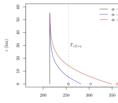
Figure 2 shows solutions of Eq. (21) for different values of α. In the limit of an almost completely transparent at-mosphere (α→0), the whole atmosphere attains one single equilibrium temperature (Eq. 22) and the surface temperature attains the effective equilibrium radiative temperature of the planet (Eq. 20). Note that the vertically continuous model de-rived here can be interpreted as a generalization of a discrete-layer model (see Appendix B).
200 250 300 350
0
10
20
30
40
50
60
T (K)
z
(km)
α = 0 α = 2 α = 6
Teff,eq
Figure 2.Vertical temperature profiles of a grey atmosphere in
overall equilibrium for different absorptivitiesα. The latter cor-responds toαoin the window-grey model withβw=0.Teff,eq= 255 K. The circles atz=0 denote the corresponding surface tem-peratures. Note that the vertical coordinatezis only approximate height, calculated fromh with a constant scale heightH=8 km such thath=1−e−z/H.
3 The window-grey atmosphere model
In reality, the atmosphere is not uniformly opaque for LW radiation, as within the grey approximation, but interacts dif-ferently with LW radiation of different wavelengths. To ac-count for this in the simplest possible way, we extend the grey model (Sect. 2) by splitting the total LW radiation F
into two separate LW bands: an opaque bandF1=O with opacityαo>0, and a completely transparent (window) band
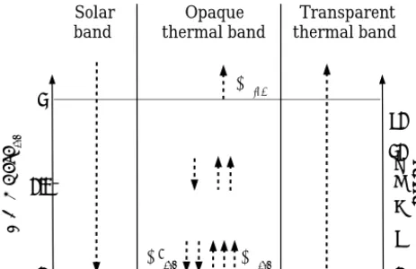
F2=W with opacityαw=0. Withβw=1−βodescribing the fraction of LW radiation from the surface which is di-rectly emitted to space, the resulting window-grey model has only two parameters:αo andβw. Thereby βw is iden-tical to the so-called transparency factorG in Thomas and Stamnes (1999), but independent of temperature in our case as we neglect Wien’s law. This approach represents the so-called window-grey or one-band Oobleck case of a multi-band model (Sagan, 1969; Pierrehumbert, 2010). In contrast to the grey-atmosphere model, the window-grey model al-lows for the existence of a spectral window, which can be interpreted as an idealization of the region between 8 and 12 µm in the Earth’s atmosphere (Fig. 1b). The window-grey model is depicted in Fig. 3.
S W O↑
toa
O↑ srf Solar
band thermal bandOpaque thermal bandTransparent
O↓ srf
h
=
1
p
/psr
f
0 0.5
1
z
(
km
)
0 4 2 6 8 10 20∞
Figure 3.Sketch of the window-grey atmosphere model.S: solar
radiation absorbed at the surface.O: radiation in the opaque LW band (↑: upwelling,↓: downwelling, srf: surface, toa: top of the at-mosphere).W: radiation emitted from the surface in the transparent LW band (atmospheric window).p: pressure. Interpreting the num-ber of arrows in the opaque LW band as proportional to the radiative flux, the illustrated case corresponds to an equilibrated atmosphere withαo=4.
dO↑(h) dh =
σ T(h)4(1−βw)−O↑(h)αo, (24)
the energy balance equation reads
2oσ T(h)4(1−βw)=o(O↑(h)+O↓(h)), (25)
and the surface emission in the opaque band is
Osrf↑ = (1−βw)σ Tsrf4 . (26)
Equations (24)–(26) can be solved analogously to the cor-responding equations describing the grey case (Eqs. 4, 6, and ). This leads to the quasi-instantaneous atmospheric temper-ature profile of the window-grey model. It is
T(h)=Tsrf 4
s
αo(1−h)+1
αo+2
. (27)
Comparison with Eq. (14) reveals that, with the same sur-face temperature prescribed as lower boundary condition, the vertical temperature profiles in the grey and in the window-grey case are identical for αo=α; the factor (1−βw) in Eqs. (24)–(26) has cancelled.
To determine the overall equilibrium state, the surface en-ergy balance needs to be incorporated. In overall equilibrium it is
S+Osrf,eq↓ =Osrf,eq↑ +Weq (28)
where
Weq = βwσ Tsrf,eq4 . (29)
Here we omitted the indices denoting the orientation and vertical position ofW (as we already did forS) because the only radiation in the window band is the one emitted upward from the surface, andW remains unchanged throughout the atmosphere becauseαw=0.
With derivations analogous to the grey case (Sect. 2), one arrives at simple expressions for the overall equilibrium state. The surface temperature for the window-grey model in over-all equilibrium is
Tsrf,eq=Teff,eq 4
s
αo+2
αoβw+2
. (30)
The corresponding vertical temperature profile reads
Teq(h)=Teff,eq 4
s
αo(1−h)+1
αoβw+2
, (31)
which implies for the TOA temperature
Ttoa,eq=Teff,eq 4
s
1
αoβw+2
. (32)
The TOA temperature, sometimes called the skin temper-ature (Goody and Yung, 1989; Pierrehumbert, 2010), can be thought of as the temperature an infinitely thin air layer above the atmosphere would have in radiative equilibrium. Obvi-ously, with βw=0 Eqs. (30)–(32) are reduced to the grey case (compare Eqs. 21–23).
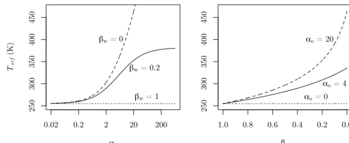
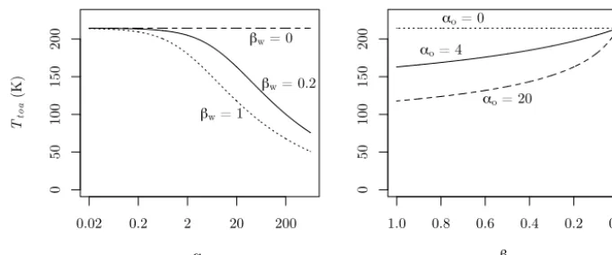
Equation (30) implies that an increased absorber amount leads to an increased equilibrium surface temperature (Fig. 4), independent of whether the added molecules absorb in the already opaque part of the LW spectrum (increasing
αo) or in the window region (decreasingβw, that is, “closing the atmospheric window”). In the following section we dis-cuss the sensitivity of atmospheric temperatures to the model parameters.
4 The mechanisms of CO2-induced
middle-atmosphere cooling
With the window-grey radiation model we are now equipped to investigate the physical essence of CO2-induced MA cool-ing. In the window-grey model, the response of temperature to changes in the parameters can be quantified with partial derivatives. The different effects of CO2-induced MA cool-ing can thereby be separated in a formal way. We present such an approach in Appendix C, but constrain the discus-sion in the following main text largely to the undifferentiated equations.
4.1 The blocking effect
250
300
350
400
450
αo Tsr
f
(K)
0.02 0.2 2 20 200
βw = 1
βw = 0.2 βw = 0
1.0 0.8 0.6 0.4 0.2 0.0
250
300
350
400
450
βw Tsr
f
(K)
αo = 0
αo = 4
αo = 20
250
300
350
400
450
αo Tsr
f
(K)
0.02 0.2 2 20 200
βw = 1
βw = 0.2 βw = 0
1.0 0.8 0.6 0.4 0.2 0.0
250
300
350
400
450
βw Tsr
f
(K)
αo = 0
αo = 4
αo = 20
Figure 4.The dependence of the overall equilibrium surface temperature on the parametersαoandβwin the window-grey model (Eq. 30).
βw=0 corresponds to the grey case.Teff,eq=255 K.
the optically thicker atmosphere, less upwelling radiation in the non-window part of the spectrum reaches high altitudes. The temperature at the TOA must thus be lower because, as follows from Eq. (25),
Ttoa= 4
s
Otoa↑
2σ(1−βw). (33)
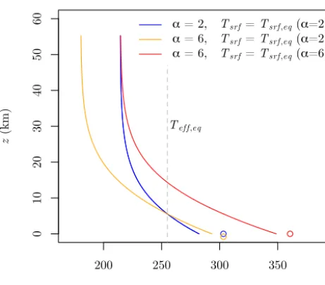
We first investigate the situation in which the assump-tion of thermal equilibrium is kept for the atmosphere but dropped for the surface. This is a reasonable assumption be-cause the atmosphere adjusts quickly to energetic changes (on the order of months) while the response of the ocean-dominated surface is very slow (including decadal and cen-tennial timescales). In reality, convection closely couples the surface with the troposphere, hence a change in green-house gases first affects the middle atmosphere, after which the slow surface-troposphere system adjusts. In the radiation model we represent this timescale separation by letting the atmosphere respond while keeping the surface temperature constant. The temperature profile for this quasi-instantaneous response is given by Eq. (27) which is valid even if the sur-face is not in thermal equilibrium. Fig. 5 shows the verti-cal temperature profile before (blue curve) and after (orange curve) increasingαin the grey case (for whichαcorresponds toαowithβw=0).
Insertingh=1 in Eq. (27) we arrive at the corresponding quasi-instantaneous TOA temperature:
Ttoa=Tsrf 4
s
1
αo+2
. (34)
Equation (34) implies a cooling at the TOA for increased
αo. Furthermore, Eq. (27) implies that at a certain heighthˆfast the sign of the fast temperature response due to added green-house gases reverses. It is
ˆ hfast=
1
2. (35)
This implies that at first the upper half of the atmosphere (with respect to mass) is cooled while the lower half is warmed.
Both the upper-level cooling and the lower-level warming are due to enhanced blocking, that is, a reduced mean free path of LW radiation in response to increased absorptivity. In radiative equilibrium, the emission, determined by the local temperature, and the absorption of radiation are locally bal-anced. In the upper atmosphere, where downwelling radia-tion is subordinate, the upwelling radiaradia-tion received from be-low comes from higher (and thus colder) levels when the ab-sorptivity of the atmosphere is increased. Consequently, the air cools until emission and absorption are in balance again. In contrast, in lower levels near the ground, where most of the absorbed upwelling radiation comes directly from the surface (with a fixed temperature), the increased absorptivity mostly affects the downwelling radiation which now comes from lower (and thus warmer) levels, resulting in warming.
200 250 300 350
0
10
20
30
40
50
60
T (K)
z
(km)
α = 2, Tsrf = Tsrf,eq (α=2)
α = 6, Tsrf = Tsrf,eq (α=2)
α = 6, Tsrf = Tsrf,eq (α=6)
Teff,eq
Figure 5. Vertical temperature profiles of a grey atmosphere for
two equilibrium states and one transient state. While the blue and red curves show the same equilibria as the corresponding curves in Fig. 2, the orange curve shows the transient state that occurs after switching from α=2 toα=6, directly after equilibration of the atmosphere but withTsrfstill unchanged. Againαcorresponds toαo in the window-grey model withβw=0.Teff=255 K. The circles at z=0 denote the corresponding surface temperatures. Note that the vertical coordinatezis only approximate height, calculated fromh with a constant scale heightH=8 km such thath=1−e−z/H.
would force the OLR to increase as well, the OLR does not change when CO2is increased, even though the temperature is increased throughout the atmosphere.
The situation is different in the presence of an atmospheric window where a part of the surface radiation is emitted di-rectly to space, bypassing the atmosphere. An atmospheric window implies a reduced sensitivity of the surface temper-ature to the state of the atmosphere (its absorptivity in the opaque band and the corresponding temperature profile, see Eq. 30) because the radiation in the opaque LW band be-comes less important in the surface energy budget (Eq. 28) with increasing window size. Consequently, in the presence of an atmospheric window, a permanent cooling at the TOA remains after the surface has equilibrated (Eq. 32).
It becomes evident from Eq. (32) that, in contrast to the surface, at the TOA the sign of the temperature response de-pends on the spectral property of the added absorbers: if they absorb in the already opaque part of the LW spectrum (in-creasingαo),Ttoa,eq is decreased (MA cooling), but if they absorb in the transparent part of the LW spectrum (decreas-ingβw, that is, “closing the atmospheric window”),Ttoa,eqis increased (MA warming) (Fig. 6).
In fact, decreasing βw leads in overall equilibrium to a temperature increase at every height in the atmosphere (Fig. 7, top). In contrast, if molecules absorbing in the opaque
LW band are added, the sign of the equilibrium temperature response reverses at a certain heighthˆ
eq, with cooling above and warming below (see Eq. C6; Fig. 7, bottom):
ˆ
heq(βw)=1−βw
2 . (36)
Forβw=0, that is in the grey case,hˆeq becomes 1 (the corresponding geometric heightzˆeq becomes ∞), meaning that no cooling takes place.
We term the above described cooling in the upper parts of the atmosphere theblocking effectof CO2-induced MA cool-ing. This presupposes that the main consequence of adding CO2 to the atmosphere is, in terms of the window-grey model, an increase ofαorather than a decrease ofβw. The permanent component of this effect, thepermanent blocking effect, is revealed by Eqs. (31) and (32). It has to be distin-guished from the instantaneous blocking effect, which con-sists of the permanent blocking effect and a transient com-ponent. The instantaneous blocking effect can be observed when atmospheric CO2is altered but when the surface tem-perature has not yet adjusted to the forcing (which is to some extent also the case for present-day Earth). In the grey model the blocking effect is only a transient phenomenon: the entire atmosphere has warmed (except at the TOA) after the surface has equilibrated. In the window-grey model the blocking ef-fect has a permanent component that persists after the surface has adjusted.
The blocking effect can be understood in terms of the in-terplay between the sensitivity of the surface temperature to greenhouse-gases on the one hand and the blocking of up-welling LW radiation by greenhouse gases on the other hand: while an atmospheric window diminishes the sensitivity of the surface temperature toαo(see Eq. 30), the blocking as-sociated withαois independent of the presence or width of an atmospheric window (see Eq. 27). Only in the grey case, where the sensitivity of the surface temperature is at its max-imum (Eq. 30), the surface temperature response is strong enough to compensate for the blocking effect, resulting in anαo-independent equilibrium TOA temperature (compare Eq. 32).
0
50
100
150
200
αo
Tto
a
(K)
0.02 0.2 2 20 200
βw = 0
βw = 0.2
βw = 1
1.0 0.8 0.6 0.4 0.2 0.0
0
50
100
150
200
βw
Tto
a
(K) αo = 20 αo = 4
αo = 0
0
50
100
150
200
αo
Tto
a
[K]
0.02 0.2 2 20 200
βw = 0
βw = 0.2
βw = 1
1.0 0.8 0.6 0.4 0.2 0.0
0
50
100
150
200
βw Tto
a
[K] αo = 20
αo = 4
αo = 0
Figure 6.The dependence of the overall equilibrium temperature at the top of the atmosphere on the parametersαoandβwin the
window-grey model (Eq. 32).βw=0 corresponds to the grey case.Teff,eq=255 K.
4.2 The indirect solar effect
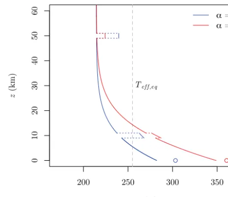
On Earth not all solar radiation transects the air unhindered, but some is absorbed within the atmosphere and leads to increased temperatures, particularly in the upper parts of the ozone layer. The solar heating can be incorporated into Eq. (25) as an additional termS∗(h):
2oσ T∗(h)4(1−βw)=o
O↑(h)+O↓(h)+S∗(h). (37)
Equation (37) is similar to Eq. (6.15) in Neelin (2011), ex-cept that Neelin considers only the grey case (βw=0) and neglects the downwelling LW radiation, constraining the va-lidity of the equation to the vicinity of the TOA.
Assuming that solar heating is confined to an infinitesi-mally thin layer ath=h0, such that the equilibrium temper-ature everywhere else remains unchanged and, thus,O↑(h0) andO↓(h0) are not affected by the additional term, one ar-rives at
T∗(h0)4=T(h0)4+ s ∗(h0)
αo(1−βw), (38)
where T(h0) is the solution of Eq. (37) with S∗(h0)=0, that is, the window-grey solution of Eq. (25), ands∗(h0)= S∗(h0)/(2σdh) .
Equation (38) reveals the following: given that due to an additional term in the local energy budget the atmospheric temperature at some height is deflected from the window-grey solution, increasing the amount of LW absorbers in the atmosphere results in a relaxation of the temperature towards the window-grey solution. This holds both for increasingαo and for decreasingβw. It must be kept in mind though that the window-grey solution itself depends onαoandβw(Eq. 31), making the relaxation towards the window-grey solution an additional effect. Figure 8 illustrates the indirect solar effect for the grey case (i.e., forβw=0).
If the additional terms∗is positive, as it is the case for the absorption of solar radiation by ozone, increasing the emis-sivity either by increasingαoor by decreasingβwresults in
local cooling. We call this effect theindirect solar effect of CO2-induced MA cooling. The term “indirect” reminds us that this effect is not due to any change in solar heating rates as might be caused by a change in ozone concentrations. In-stead, the mere presence of solar absorption is a prerequisite for this effect. Like the permanent blocking effect, the indi-rect solar effect is still at work when the system has reached the new (more opaque) overall equilibrium. Note that the indirect solar effect would also manifest if the opacity was changed only locally. This is not the case for the blocking effect, where integration over a finite layer with perturbed opacity is needed.
5 Effect strengths
An essential question so far unanswered is how strong the above derived effects are compared to each other. In this sec-tion we apply a complex atmospheric model to give a quan-titative answer to this question, and we discuss the implica-tions and limitaimplica-tions of the window-grey model in the light of these results.
spatio-706 H. F. Goessling and S. Bathiany: Why CO2cools the middle atmosphere
200 250 300 350
0
10
20
30
40
50
60
T (K)
z
(km)
αo = 4 βw = 0.3
βw = 0.1
Teff,eq
200 250 300 350
0
10
20
30
40
50
60
T (K)
z
(km)
βw = 0.2
αo = 2 αo = 6
Teff,eq
200 250 300 350
0
10
20
30
40
50
T (K)
z
(km)
βw = 0.3
βw = 0.1
Teff,eq
200 250 300 350
0
10
20
30
40
50
60
T (K)
z
(km)
βw = 0.2
αo = 2 αo = 6
Teff,eq
Figure 7.Vertical temperature profiles in overall equilibrium for
the window-grey case withTeff,eq=255 K for different combina-tions of the parametersαoand βw (Eq. 31). The circles atz=0 denote the corresponding surface temperatures. Note that the verti-cal coordinatezis only approximate height, calculated fromhwith a constant scale heightH=8 km such thath=1−e−z/H.
temporal resolution. The radiative transfer scheme used in ECHAM6, which employs 16 LW bands, has been shown to give instantaneous clear-sky responses to greenhouse-gas perturbations in close agreement with accurate line-by-line calculations (Iacono et al., 2008). To adequately resolve the middle atmosphere, we have used the T63L95 configuration with relatively coarse (∼2◦) horizontal but high (95 levels, top at 0.01 hPa) vertical resolution. The distribution of ozone is prescribed by a climatology.
The ocean and sea ice have been treated in a simple way similar to the approach of Dickinson et al. (1978). The ocean surface temperature and sea ice concentration and thickness are prescribed with a realistic seasonal and spatial pattern
de-200 250 300 350
0
10
20
30
40
50
60
T (K)
z
(km)
α = 2
α = 6
Teff,eq
Figure 8.Vertical temperature profiles of a grey atmosphere that is
additionally locally heated (e.g., by absorption of solar radiation) at two heights within the atmosphere. Apart from the heights at which the profiles are locally deflected due to additional heating, the blue and red curves show the same grey equilibria as the corresponding curves in Fig. 2. Againαcorresponds toαo in the window-grey model withβw=0 . The heights at which additional heating occurs (z1≈10 km,z2≈50 km) and the magnitude of the additional heat-ing terms (specified such that the temperature rise is 25 K forα=2 at both heights) are more or less arbitrarily chosen to demonstrate the effect.Teff,eq=255 K. The circles at z=0 denote the corre-sponding surface temperatures. Note that the vertical coordinatez is only approximate height, calculated fromhwith a constant scale heightH=8 km such thath=1−e−z/H.
rived from observations. After every year the ocean surface temperature pattern is updated uniformly according to the to-tal energy imbalance integrated over the global ocean surface (including sea ice) and over the year, using a heat capacity that corresponds to a 50 m thick mixed-layer ocean. Despite changing temperatures, the sea ice state pattern is not up-dated, leading to discrepancies between the sea ice and ocean states. This procedure also suppresses further changes to the surface temperature pattern, such as polar warming amplifi-cation. However, this allows for a rapid thermal equilibration of the surface with an exponential timescale of ∼3 years, serving the purpose of this paper where the focus is on the global-mean response.
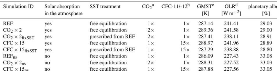
sensitiv-Table 1.ECHAM6 simulations.
Simulation ID Solar absorption SST treatment CO2a CFC-11/-12b GMSTc OLRd planetary albedo
in the atmosphere [K] [W m−2] [%]
REF yes free equilibration 1× 1× 287.14 241.41 29.03
CO2×2 yes free equilibration 2× 1× 289.36 241.58 29.00
CO2×2fixSST yes prescribed from REF 2× 1× 287.41 238.11 28.91
CFC×15 yes free equilibration 1× 15× 288.97 241.96 28.89
CFC×15fixSST yes prescribed from REF 1× 15× 287.29 238.88 28.80
REFns no free equilibration 1× 1× 286.09 227.43 33.08
CO2×2ns no free equilibration 2× 1× 288.31 227.52 33.03
CFC×15ns no free equilibration 1× 15× 287.88 227.56 33.05
a1×: CO
2=280ppmv; 2×: CO2=560ppmv,b1×: CFC11=0.2528 ppbv, CFC12=0.4662 ppbv; 15×: CFC11=3.792 ppbv, CFC12=6.993 ppbv,cglobal annual-mean
near-surface air temperature,doutgoing longwave radiation at the top of the atmosphere.
ity simulations. In two of these the ocean is allowed to attain a new equilibrium, either with the CO2 concentration dou-bled or with the Chlorofluorocarbon (CFC-11 and CFC-12) concentrations increased by the factor 15, chosen such that the surface warming is similar compared to the case of CO2 doubling. The other two sensitivity simulations are identical with the previous two, except that the SSTs are prescribed from the reference simulation.
In another set of three simulations the absorption of so-lar radiation by all atmospheric gases (but not cloud droplets or ice) is turned off. This set also includes a reference sim-ulation and two sensitivity simsim-ulations with increased CO2 and CFC concentrations. In these, the SSTs are again al-lowed to run into equilibrium. All simulations are conducted over 22 years, but only the last 10 years are used to com-pute averages for the analysis because it takes a few years (in our setup) until an equilibrium is reached. This experi-mental design allows us first to demonstrate the dependence of MA temperature changes on the spectral properties of the added absorbers: CFCs absorb mainly in the spectral win-dow of the Earth’s atmosphere, whereas CO2absorbs mainly at wavelengths where the atmosphere is already relatively opaque. Second, we can quantify the effect strength for the two permanent effects by which CO2cools the MA, deduced above with the window-grey model, and investigate how at-mospheric temperatures respond to the slow surface adjust-ment.
When the absorption of solar radiation by gases is switched off, the total short-wave absorption in the atmo-sphere drops from 75 W m−2 in REF to only 13 W m−2 in REFns, the residue being due to absorption by tropospheric clouds. The lack of short-wave heating due to ozone leads to a strong cooling of the MA. The local temperature maxi-mum around the stratopause completely disappears and tem-peratures drop to∼160 K in the upper stratosphere and in the mesosphere, in agreement with previous studies (Man-abe and Strickler, 1964; Fels et al., 1980). Tropospheric tem-peratures are only slightly reduced by ∼1 K (Table 1 and Fig. 9 left). This small temperature change is the result of
a compensation of different effects. After removing the ab-sorption of solar radiation, more short-wave radiation propa-gates downwards through the atmosphere. A part of the pre-viously absorbed radiation is then scattered and the plane-tary albedo increases from 29 to 33 %. The rest is partly ab-sorbed in the troposphere by cloud droplets and ice crystals, and partly reaches the Earth’s surface where the downwelling solar radiation is increased by 42 W m−2. This instantaneous redistribution of short-wave fluxes tends to warm the surface. However, the large cooling in the MA that follows also leads to a decreased downwelling long-wave radiation at the sur-face which has a cooling effect. To this extent, our result is in line with previous simulations that quantified the effects of stratospheric ozone removal (Ramaswamy et al., 1992; Hansen et al., 1997; Forster et al., 1997a; Stuber et al., 2001). In contrast to these studies, we still keep ozone as a green-house gas as only its short-wave absorption is removed. How-ever, this is not a very important difference as the short-wave effect of ozone has been shown to be more important than the long-wave effect (Dickinson et al., 1978; Ramaswamy et al., 1992; Forster et al., 1997a). A similar cancellation of short-and long-wave effects on the surface temperature seems to hold for other gases. The lack of absorption by water vapour further shifts the heating from the lower troposphere to the surface, without much impact on the surface temperature. An additional effect that might be of relevance for the sur-face cooling in these simulations is the reduction in specific humidity due to the atmospheric cooling.
by the window-grey model, results from the temperature dependence of the moist-adiabatic lapse rate (the so-called lapse-rate feedback) and is thus related to convective pro-cesses. Somewhat above the tropopause the temperature re-sponse changes sign. In agreement with earlier studies (Man-abe and Wetherald, 1967; Fels et al., 1980), the cooling then increases with height and assumes a maximum cooling by 11.6 K around the stratopause region.
Adding CFCs instead of CO2 results (by design) in a similar tropospheric response with a near-surface warming by 1.8 K, but temperatures in the MA remain virtually un-changed (Fig. 9 middle, black solid curve). Again, this result agrees with previous studies (Dickinson et al., 1978; Forster and Joshi, 2005). However, our simulations also show that the near-zero MA temperature change is due to a cancella-tion of two effects: the indirect solar effect is not wavelength dependent. More absorbers increase emission more strongly than they increase absorption, thereby reducing the relative importance of the solar heating term (Sect. 4.2). This sug-gests that another effect counteracts the cooling from the in-direct solar effect. The above considerations based on the window-grey model suggest that this counteracting warm-ing effect can be interpreted as aninverse blocking effect: in-stead of making the already opaque part of the spectrum even more opaque, which mainly happens when CO2 is added, the increase of CFC concentrations acts to narrow the atmo-spheric window, corresponding to a decrease of βw in the window-grey model (Figs. 7 and 6 top). In fact, the situa-tion corresponds not only to a decrease of βw, but also to a simultaneous decrease of αo because the average opacity of what should be translated into the single opaque band of the window-grey model is decreased by the inclusion of the CFC-affected – still relatively transparent – parts of the pre-vious window band. Overall, the MA is more strongly sub-jected to the radiation from the warm surface.
In the case without solar absorption by gases within the at-mosphere, adding CO2or CFCs results in similar responses in the troposphere, but markedly different responses in the MA (Fig. 9 middle, dashed curves): while the cooling in response to CO2 is roughly halved, the previously neutral response to CFCs turns into a substantial warming by up to 3.5 K. These results are consistent with the interpretation that the cooling due to the indirect solar effect has been pre-cluded, leaving only the response due to the blocking effect (in the CO2case) and the inverse blocking effect (in the CFC case).
Under the assumption of linearity, this allows us to esti-mate the fractional contributions of the two permanent ef-fects to MA cooling (Fig. 9 right). According to our results the indirect solar effect contributes up to∼70 % to the total permanent cooling around the stratopause where solar heat-ing is strongest. Outside this region the blockheat-ing effect gains importance and begins to dominate the cooling in the middle stratosphere and the middle mesosphere. The assumption of linearity is rather crude, so these estimates should be taken
with a grain of salt. In fact, it is probably not possible to make a completely clean quantitative distinction, as the for-mal analysis in Appendix C3 suggests.
The window-grey model also suggests a transient MA cooling that adds to the permanent cooling before the surface temperature has adjusted to the changed radiative forcing. We can investigate this effect with the remaining two sim-ulations where the greenhouse gases are perturbed but SSTs are fixed to the reference state (Table 1). Interestingly, the ini-tial MA responses (Fig. 9 middle, dotted curves) are nearly identical with the corresponding equilibrium responses (solid curves) above∼20 km. This means that, given a fixed at-mospheric composition in terms of well-mixed greenhouse gases, MA temperatures are almost independent of the sur-face temperature.
In the window-grey model the increased surface temper-ature entails increased upwelling LW radiation in both the window and the opaque band. In contrast, the additional upwelling LW radiation of approx. 3.5 W m−2 (beyond the tropopause) in CO2×2 compared to CO2×22fixSSTis con-strained to transparent parts of the spectrum and has thus no impact on MA temperatures. This result is not specific to our simulations and in line with previous studies. In particular, Forster et al. (1997b) use a radiative-convective model and show that the radiative forcing by CO2depends on the defini-tion of the tropopause. While this affects the response of the surface-troposphere system, the temperature profile above is not affected by the definition of the tropopause (see their Fig. 8a). A similar argumentation applies to changes in sur-face albedo: the latter would affect the sursur-face temperature directly and lead to an adjustment of the troposphere, but the effect decays with height (Manabe and Wetherald, 1967, Fig. 19). Hence, the temperature in the MA appears to be di-rectly determined by the actual atmospheric composition and not by the history of this composition (i.e., the concentration scenario) and associated surface temperature changes.
A possible explanation for the discrepancy between com-plex models and the window-grey model regarding the slow MA adjustment, as well as other limitations of the window-grey model are discussed in the following section.
5.2 Limitations of the window-grey model
Given the simplicity of the window-grey model, quantita-tive statements are difficult to make and the cases shown in Figs. 2, 5, 7, and 8 are quantitatively unrealistic. Here we nevertheless attempt to derive some crude estimates based on the window-grey model, and discuss discrepancies to ECHAM6 in the light of obvious limitations of the window-grey model.
150 200 250 300
0
20
40
60
80
T (K)
z
(km)
REF REFns
-10 -5 0 5
0
20
40
60
80
ΔT (K)
z
(km)
CO2x2 - REF CFCx15 - REF
CO2x2ns - REFns
CFCx15ns - REFns
CO2x2fixSST - REF
CFCx15fixSST - REF
0 20 40 60 80 100
0
20
40
60
80
Percentage permanent cooling for CO2x2
z
(km)
Permanent blocking effect
Indirect solar effect
Figure 9.Results obtained with ECHAM6 coupled to a simplistic ocean model to allow for rapid thermal adjustment of the surface. Left:
global annual-mean equilibrium temperature profiles for two reference runs under pre-industrial external forcing, with (solid; REF) and without (dashed; REFns) absorption of solar radiation in the atmosphere. Middle: temperature difference to the corresponding reference runs in response to increased CO2or CFC concentrations (simulation IDs are explained in Table 1). Right: percentage of the permanent cooling effect in response to CO2 doubling from the blocking and indirect solar effects, estimated by dividing CO2×2ns−REFns by CO2×2−REF. Note that the vertical coordinatezis only approximate height, calculated fromhwith a constant scale heightH=8 km such thath=1−e−z/H.
∂Ttoa,eq
∂αo
/∂Tsrf,eq ∂αo
= −1 2
T
srf,eq
Ttoa,eq
3
βw 1−βw
. (39)
One can now insert typical temperatures prevailing at the Earth’s surface (∼290 K) and at the mesopause (∼180 K), and an estimate ofβw≈10–20 % (the actual values depend on the optical thickness threshold used to deriveβwfrom the continuous absorption spectra, compare Fig. 1b–c). This sim-ple calculation yields response ratios of approximately only (−0.2)−(−0.5), i.e., a larger temperature change at the sur-face than in the MA. This result stands in sharp contrast to ECHAM6 where the surface warms much more than the MA cools by the permanent blocking effect.
Probably the main reason for this discrepancy is that the effective width of the atmospheric window is very different for the atmosphere as a whole and for the atmosphere beyond the tropopause alone. The width of the atmospheric window is however crucial for the atmospheric temperature profile and the strength of the MA cooling effects both in absolute and relative terms. Considering thatβw≈90–95 % is more representative for the largely water-free atmosphere beyond the tropopause (compare Fig. 1), Eq. (39) yields a response ratio of (−20)−(−40), which is in much better agreement with the ECHAM6 results.
Regarding the transient component of the MA cooling, the window-grey model predicts that the transient tempera-ture adjustment decays with height (see also Appendix C2, Eq. C10), but it fails to explain the virtual absence of a tran-sient MA adjustment in ECHAM6. This might be linked to another effect neglected in the window-grey model, namely the water vapour feedback. Higher tropospheric temperatures imply higher water vapour concentrations, leading to a pro-nounced temperature dependence of the atmospheric
opac-ity. The increased opacity as a result of tropospheric warm-ing entails that asecondary blocking effectmay counteract the slow reduction of the initial MA cooling associated with the transient component of the blocking effect seen in the window-grey model. We therefore speculate that the water vapour feedback might play a role to explain the apparent in-sensitivity of MA temperatures to the surface temperature by redirecting changes in upwelling LW radiation to parts of the spectrum that are transparent in the MA.
Moreover, the height-dependent width of the atmospheric window acts in concert with the effect of convection. Convection acts to reduce the lapse rate considerably, to ∼6.5 K km−1in the current climate, leading to an approxi-mately constant lapse rate in the troposphere (e.g., Manabe and Wetherald, 1967). The appearing radiative-convective equilibrium in the troposphere is associated with an upward heat transport and increased temperatures in the free tropo-sphere and decreased temperatures at (and close to) the sur-face. The redistribution of heat from the surface to the up-per troposphere by convection thus bypasses the lower levels where the atmospheric window is small. Tropospheric con-vection is thus an efficient process to attenuate the surface response to greenhouse forcing, but convection is neglected in the window-grey model.
It is tempting to apply the window-grey model only to the MA, prescribing the upward radiative flux in the opaque ther-mal band (O↑) at the tropopause as a lower boundary condi-tion. The omission of the troposphere would have the advan-tages that convection does not play a significant role anymore and that the complex influence of the unevenly distributed at-mospheric water (in all its aggregate phases) is strongly di-minished.
Trans-ferred to the window-grey model, this yields
T(h)= 4
v u u t
Otp↑ σ(1−βw)
αo(1−h)+1
αo(1−htp)+2
. (40)
One could now investigate how changes inOtp↑ orhtp af-fect the MA, but this would not be very conclusive because
Otp↑ and htp respond in a complex manner to changes in greenhouse-gas forcing. One could also follow a hybrid ap-proach by using values derived from a complex model like ECHAM6 forOtp↑ andhtp. However, in particular the deriva-tion of Otp↑ from a multi-band LW scheme would not be straightforward. Moreover, the ECHAM6 results show that above a certain height the temperature profile will not re-spond to changes in the troposphere. In other words,Otp↑and
htpappear to change in such a way that the temperature pro-file above remains the same. Overall, applying the window-grey model only to the MA appears not to add to our expla-nation of why CO2cools the MA.
6 Summary and conclusions
In this article we explain a well-known phenomenon that is central to our general understanding of climate change – cooling of the middle atmosphere (MA) by CO2– in a simple but physically consistent way. We do so by applying a verti-cally continuous window-grey radiation model to the phe-nomenon. This way it is possible to distinguish two main ef-fects by which CO2cools the MA.
First, enhanced blocking of upwelling LW radiation oper-ates towards lower MA temperatures. In principle, this block-ing effecthas a transient component due to the slow warming of the surface. This adjustment leads to intensified upwelling LW radiation and tends to reduce the initial MA cooling in the window-grey model. While these effects exactly compen-sate each other in a grey atmosphere, leading to an equilib-rium TOA temperature that is independent of the atmospheric opacity, the blocking of upwelling LW radiation outweighs in the presence of a spectral window because of the reduced sur-face temperature sensitivity, leaving lower equilibrium tem-peratures above a critical height after the adjustment. Hence, the blocking effect is permanent because the Earth’s atmo-sphere is not grey, i.e., uniformly opaque for LW radiation at any wavelength, but absorbs and emits LW radiation with varying intensity depending on wavelength. The introduction of a spectral window into an otherwise uniformly opaque at-mosphere is the simplest possible means to capture the effect in a physical model.
The second permanent effect of CO2-induced MA cooling is the indirect solar effect. It owes its existence to the fact that there are heat sources within the atmosphere in addi-tion to LW radiaaddi-tion, most importantly solar radiaaddi-tion that is absorbed in particular in the vicinity of the stratopause
by ozone. The additional heating term causes a deviation of the temperature profile from the window-grey solution. The strength of this deviation depends on the abundance of LW absorbers because the relative importance of the constant ad-ditional heating term in the local energy budget decreases with increasing LW absorber abundance.
While the window-grey model allows for a fully analyt-ical treatment of CO2-induced MA cooling, it is not well suited to constrain the relative effect strengths. Uncertainties are large because the window-grey model entails a number of gross simplifications, including in particular: the assump-tion of vertically well-mixed greenhouse gases (violated in particular by water vapour); the simplistic LW band struc-ture; and the neglect of vertical heat transport by convection (and conduction at the surface). Additional simplifications are the following: the neglect of Wien’s law; the two-stream approximation; the neglect of the horizontal dimensions and the associated differential heating and atmospheric dynam-ics (including gravity waves); the neglect of chemical pro-cesses; the implicit treatment of solar radiation; the neglect of clouds, aerosols, and scattering in general; and the assump-tion of local thermodynamic equilibrium that does not hold in the upper mesosphere and beyond. Most of these factors are discussed for example in Pierrehumbert (2010), and those specific to the mesosphere are reviewed in Mlynczak (2000). Therefore, to quantify the effect strengths and to comple-ment the insights gained from the window-grey model, we have conducted simulations with a much more complex at-mospheric model. The results indicate that the two perma-nent effects are similarly important, with the indirect solar effect dominating around the stratopause and the blocking effect dominating away from the stratopause. The window-grey model also predicts a slow (re-)warming throughout the atmosphere in response to the slow surface warming. How-ever, this transient effect is negligible in the MA according to the simulations with the complex model, pointing to the limitations of the window-grey model.
This article is meant to consolidate our understanding of why CO2 cools the middle atmosphere by filling a gap between reality and complex atmospheric models on the one side and somewhat scattered heuristic arguments on the other. The reconsideration of CO2-induced MA cooling as put forward here has a distinct educational element, with the potential to convey the physical essence of the involved mechanisms to a broader audience.
7 Data availability
Appendix A: An analogy for the blocking effect
While the explanations based on the window-grey model in-volve mathematical formalism, the following analogy may facilitate an intuitive understanding for the permanent and transient components of the blocking effect.
Consider a building that is heated at a constant rate from inside. In steady state there is a higher temperature inside the building compared to the fixed exterior temperature. The walls of the building represent an analogy to the Earth’s at-mosphere, with the outer surface as the top of the atmosphere and the inner surface as the atmosphere close to the Earth’s surface. The temperature at the outer wall surface is higher than the exterior temperature and the temperature at the inner wall surface is somewhat lower than the interior (room) tem-perature. These temperature differences maintain an export of heat at the same rate at which the interior is heated. In the following we assume that the walls have negligible heat ca-pacity whereas the interior reacts more inertly to disturbances due to a non-zero heat capacity.
We first assume that the building is insulated equally well everywhere (corresponding to the grey case), resulting in a uniform temperature of the outer surface. If now the heat resistance of the walls is instantaneously increased, at first the outer surface temperature drops and the inner surface temperature rises, while the interior temperature is still un-changed. In this situation less heat escapes from the building than is released by the heating system. The imbalance leads to a slow ascent of the interior temperature that continues un-til the outer surface temperature returns to its original value. The initial cooling of the outer surface temperature is anal-ogous to the quasi-instantaneous cooling that occurs in the upper half of the atmosphere in the grey model; the cooling is only transient and has no permanent component.
Assuming instead that there are parts of the building enve-lope that are more weakly insulated than the remainder, as is typically the case with windows, the outer surface tempera-ture in equilibrium is higher at the windows than it is at the walls, and a larger fraction of the total energy escapes via the windows compared to how much they contribute to the to-tal area of the building envelope. If now the heat resistance of the walls is increased, the outer surface temperature of the wall is diminished not only temporarily, but some cool-ing remains also after the interior temperature has increased to its new equilibrium value. In the new equilibrium, even more energy escapes through the windows and less through the walls. The permanent cooling of the outer surface tem-perature of the walls is analogous to the cooling in the higher atmosphere associated with the permanent blocking effect of CO2-induced MA cooling.
The main difference between the building analogy and the window-grey radiation model is that the separation between walls and windows in the former case is in geometrical space, whereas the separation into an opaque and a transparent ra-diation band in the latter case is in spectral space. Another
obvious difference is that the mechanism of energy transfer is heat conduction in the walls of a building as opposed to ra-diation in the atmosphere. Nevertheless, we reckon the anal-ogy of an insulated building as a valid means to illustrate the blocking effect of CO2-induced MA cooling.
Appendix B: Relation to discrete-layer models
Without showing derivations we point out that the vertically continuous model(s) presented in the main text can be in-terpreted as a generalization of discrete-layer models. The simplest type of the latter, a model with only one grey atmo-spheric layer, is widely used to explain the greenhouse ef-fect in a conceptual way (e.g., Pierrehumbert, 2010; Neelin, 2011). In the following we discuss only the grey case, but the window-grey case can be treated analogously.
In annlayer grey-atmosphere model with uniform layer emissivity l, from the radiative balances at every atmo-spheric layer it follows that, given an arbitrary surface tem-perature, the equilibrium temperature at layeriis
Ti=Tsrf 4
s
l(n−i)+1
l(n−1)+2
, (B1)
wherei=1 is the lowest andi=nthe highest atmospheric layer. The overall equilibrium situation is obtained whenTsrf in Eq. (B1) is replaced by the value it attains in overall equi-librium, which is
Tsrf,eq=Teff,eq 4
r
1+ n l 2−l
. (B2)
Forα/2∈Nthe vertically continuous grey model is equiv-alent to a discrete grey model withn=α/2 atmospheric lay-ers, each with emissivityl=1. The heights h that corre-spond to the discrete levelsiare then determined by
hi=
i−1 2
n . (B3)
Although providing a very suitable conceptual tool to understand the greenhouse effect, the discrete-layer grey-atmosphere model (just like its continuous analogue) obvi-ously can not explain greenhouse-gas induced MA cooling. For such an explanation it is again necessary either to troduce non-uniform opacity for LW radiation (e.g., by in-troducing an atmospheric window), or to introduce an addi-tional (solar) heating term.
Appendix C: Formal response analysis
also separate the simultaneously occurring effects of CO2-induced MA cooling in a formal way. We start without the indirect solar effect but include it into the formalism later.
In the following a responseis simply the partial deriva-tive of temperature with respect to eitherαoorβw. Different responses are discerned based on the conditions introduced into the derivatives. We distinguish between a fast (quasi-instantaneous) responseF where the surface temperature is kept fixed at its previous equilibrium value, and a subsequent slow responseSduring which also the surface attains its new equilibrium temperature. The overall equilibrium responseE
can thus be written as
E=F+S. (C1)
During the slow transition from F toE, the current re-sponse C(t) at time t deviates from E by the transient re-sponseT(t):
C(t)=E+T(t), (C2)
with
T(t)= f(t)−1
S, (C3)
where f(t)∈ [0,1] is that fraction of the slow response that has already taken effect at time t, with f(0)=0 and
f(t→ ∞)=1. The transient response is thus defined as the part of the quasi-instantaneous response that is later compen-sated by the adjustment to surface warming.
C1 Surface response
Differentiating Eq. (30) with respect toαoandβwgives the overall equilibrium responsesEαo andEβw at the surface:
Eαo,srf≡
∂Tsrf,eq ∂αo = Teff 4 4 s
αo+2
αoβw+2
1
αo+2
− βw
αoβw+2
(C4)
and
Eβw,srf≡
∂Tsrf,eq
∂βw
=−Teffαo 4
4
s
αo+2 (αoβw+2)5
. (C5)
Excluding the trivial casesαo=0 andβw=1 , Eqs. (C4) and (C5) imply that Eαo,srf>0 andEβw,srf<0. That is, the surface warms when greenhouse gases are added.
As there is by definition no fast response at the surface, i.e., Fαo,srf,Fβw,srf=0 , it is Sαo,srf=(f(t)−1)Eαo,srf and
Sβw,srf=(f(t)−1)Eβw,srf: the transient response fully com-pensates for the equilibrium response initially (wheref =0), but vanishes fort→ ∞.
C2 Atmospheric response
The temperature response of the continuous window-grey at-mosphere in overall equilibrium toαoandβw as a function of height is obtained by differentiating Eq. (31) with respect to the two model parameters, giving
Eαo(h)≡
∂Teq(h)
∂αo
=Teff,eq 4
4
s
αo(1−h)+1
αoβw+2
·
1−h
αo(1−h)+1
− βw
αoβw+2
(C6)
and
Eβw(h)≡
∂Teq(h)
∂βw
=−Teff,eqαo 4
4
s
αo(1−h)+1 (αoβw+2)5
. (C7)
Differentiating the quasi-instantaneous temperature profile given by Eq. (27) in overall equilibrium ath=1 (i.e., at the TOA) with respect to αo leads to a form that supports the interpretation of the permanent blocking effect as the inter-play between the sensitivity of the surface temperature to greenhouse-gases on the one hand and the blocking of up-welling LW radiation by greenhouse gases on the other hand:
Eαo,toa= 4
s
1
αo+2
∂T
srf,eq
∂αo
− Tsrf,eq 4(αo+2)
. (C8)
Here the surface sensitivity is represented by the minuend in the brackets whereas the blocking effect is represented by the subtrahend in the brackets.
Differentiating Eq. (27) with respect toαounder the con-straintTsrf=const and inserting Eq. (30) gives the fast tem-perature response as a function of height:
Fαo(h)≡
∂T(h)
∂αo
Tsrf=Tsrf,eq=const
=Teff,eq 4
4
s
αo(1−h)+1
αoβw+2
1
αo+(1−h)−1
− 1
αo+2
.
(C9)
Note that changing the width of the atmospheric window entails no fast response, i.e.,Fβw(h)=0.
The transient part of the response follows from Eqs. (C6) and (C9) with Eqs. (C1)–(C3) as
Tαo(h, t)≡ 1−f(t)
Fαo(h)−Eαo(h)
= 1−f(t)Teff,eq
4
4
s
αo(1−h)+1
αoβw+2
·
β
w
αoβw+2
− 1
αo+2
. (C10)
that|Tαo(h, t)|<|Eαo,srf|, that is, the transient cooling at any height in the atmosphere is always weaker than the equilib-rium warming of the surface. Note thatTβw(h, t) follows di-rectly fromEβw(h) becauseFβw(h)=0.
C3 Inclusion of the indirect solar effect
Considering overall equilibrium, and simplifying the anno-tation by leaving away h0, differentiation of Eq. (38) with respect to the two model parameters gives
E∗
αo≡
∂Teq∗ ∂αo
= Teq T∗
eq
!3
Eαo−
s∗
4T∗
eq3αo2(1−βw)
(C11)
and
E∗
βw≡
∂Teq∗ ∂βo
= Teq T∗
eq
!3
Eβo+
s∗
4T∗
eq3αo(1−βw)2
, (C12)
whereEαo andEβw are the window-grey overall equilibrium responses given by Eqs. (C6) and (C7).
To include the indirect solar effect I into the formalism of Eqs. (C1)–(C3), one can extend Eq. (C2) using Eqs. (38), (C11), and (C12) as follows:
C∗(
t)=E+XEI+I
| {z }
E∗
+T(t)+XT I(t)
| {z }
T∗(t)
(C13)
with
Iαo = −
s∗
4T∗
eq3α2o(1−βw)
, (C14)
Iβw =
s∗
4T∗
eq3αo(1−βw)2
, (C15)
XEI=
Teq
T∗
eq
!3
−1
E, (C16)
XT I(t)=
Teq
T∗
eq
!3
−1
T(t), (C17)
where the terms in Eqs. (C14)–(C16) follow naturally from Eqs. (C11) and (C12). Equation (C17) results from Eq. (C13) with the analogues of Eqs. (C11) and (C12) for the fast response (i.e., withE∗andE replaced byF∗andF)
and the definition ofT∗(t) :
T∗(t)=(1−f(t))(F∗−E∗). (C18)
The termsXEIandXT Iare interaction (or synergy) terms
that result from the fact thatE,I, andT(t) are not linearly additive. Due to these terms, the quantitative attribution of a total response to the different mechanisms is not unambigu-ously possible.
Appendix D: Supporting information on Fig. 1