International Journal of Industrial Engineering Computations 7 (2016) 309–322
Contents lists available at GrowingScience
International Journal of Industrial Engineering Computations
homepage: www.GrowingScience.com/ijiec
M-machine, no-wait flowshop scheduling with sequence dependent setup times and truncated learning function to minimize the makespan
V. Azizia*, M. Jabbarib and A. S. Kheirkhahb
aDepartment of Industrial Engineering, K. N . Toosi University of Technology, Iran, Tehran
bDepartment of Industrial Engineering, Bu-Ali Sina University, Hamedan, Iran
C H R O N I C L E A B S T R A C T
Article history: Received July 21 2015 Received in Revised Format August 16 2015
Accepted September 8 2015 Available online
September 30 2015
Recently, learning effects have been studied as an interesting topic for scheduling problems, however, most researches have considered single or two-machine settings. Moreover, learning factor has been considered for job times instead of setup times and the same learning effect has been used for all machines. This paper studies the m-machine no-wait flowshop scheduling problem considering truncated learning effect in no-wait flowshop environment. In this problem, setup time is a function of job position in the sequence with a learning truncation parameter and each machine has its own learning effect. In this paper, a mixed integer linear programming is proposed for the problem to solve such problem. This problem is NP-hard so an improved genetic algorithm (GA) and a simulated annealing (SA) algorithm are developed to find near optimal solutions. The accuracy and efficiency of the proposed procedures are tested against different criteria on various instances. Numerical experiments approve that SA outperforms in most instances.
© 2016 Growing Science Ltd. All rights reserved Keywords:
No-wait flowshop Learning effect Genetic Algorithm Simulated Annealing Truncated learning parameter
1. Introduction
Learning effect in scheduling was introduced by Biskup (1999) and Cheng and Wang (2000). In elementary scheduling systems with learning effect it is assumed that learning effects are used for job processing time. It means, in a permutation schedule the processing time of a job is a function of its position in the schedule. Also in these models learning effect was uncontrolled and with increasing the number of jobs, the processing times of the jobs at the end of schedule converge to zero. In the real world, this is an odd event. This problem is removed by Cheng et al. (2013) by adding a truncation learning parameter to classical learning model. This is a control parameter and does not allow the job time to drop to zero. This concept is new and it can be improved in many directions. The majority of the literature has focused on single or two-machines. Also, to the best of our knowledge, there is no research considered learning effect on sequence dependent setup times. The setup times are completely prone to be decreased because of human experiences. The commonly learning models use the same learning factor for machines
* Corresponding author.
that is in conflict with reality. Each machine should have different learning factor, because different people working as operators on machines. The learning effect in no-wait flowshop is another direction for developing the learning effects models.
Motivated by these observations, this paper proposes m-machine no-wait flowshop scheduling problem with sequence dependent setup times and truncated learning function to minimize the makespan in which the actual sequence dependent setup time of a job is calculated by a function of the job’s position in the schedule and a control parameter, namely truncation parameter. In this model, each machine has its own learning factor and truncation parameter. As three-machine no-wait flowshop scheduling problem is NP-hard (Rock, 1984) so the proposed m-machine no-wait flowshop scheduling problem with consideration of other mentioned assumptions, is also NP-hard.
The rest of this study is as follows: section 2 reviews the related works in the literature. Section 3 describes the introduced problem in the paper and addresses a mathematical formulation. Section 4 develops a genetic algorithm and a simulated annealing method to solve the problem. The numerical experiments are analyzed in section 5. Finally, section 6 includes conclusion and suggests some directions for further works.
2. Literature Review
As mentioned in the previous section Biskup (1999) and Cheng and Wang (2000) are pioneers in applying learning effects in scheduling problems. Since then, many works have appeared in this field of research. Most of the published papers consider simple form of scheduling flowshop problems with single or two-machines. Lee and Wu (2004) considered learning effect in two-machine flowshop scheduling problem with the criterion of minimizing completion time. Chen et al. (2006) studied two-machine flowshop scheduling problem, including learning effect with respect to two criteria: minimizing total completion time and the weighted sum of maximum tardiness. They proposed a branch and bound algorithm which was capable of solving problems with up to 18 jobs. Wang and Xia (2005) added the assumption of increasing dominance machine into the flowshop scheduling problem with learning effects. Wang and Liu (2009) developed two-machine flowshop scheduling problem with deterioration and learning effects. Wu et al. (2007) considered minimizing the maximum tardiness in two-machine flowshop scheduling problem with learning effect. The authors proposed branch and bound algorithm and a simulated annealing algorithm for solving the problem.
Eren and Gunar (2008) analyzed bi-criterion two-machine flowshop problem under learning effects to minimize makespan and weighted sum of total completion time. They proposed an integer programming model and constructed a heuristic algorithm based on tabu search.
Lee and Wu (2009) proposed a new learning model that unifies machine and human learning effects. They proved that single and m-machine flowshop problems can be solved in polynomial time. Isler et al (2012) proposed two-machine flowshop scheduling problem to minimize total earliness and tardiness penalties with learning effects assumption. They developed a mathematical formulation to reach an optimal solution for the problem. Janiak et al. (2009) studied a single processor makespan problem with learning effects and showed that the problem is strongly NP-hard. The authors developed a branch and bound algorithm and heuristic methods for solving instance problems to gain optimal and near optimal solutions.
to obtain the optimal solutions in small size instances and a genetic algorithm to obtain near optimal solutions in large scale instances.
In addition, Biskup (2008) provided a review paper of scheduling with learning effects. He classified models based on two approaches: first, position-based learning and second, sum-of-processing-time-based learning. He claimed that the first kind of learning models occurs by processing independent operations and the second type of models considers the experience factor that the workers obtain. Kunjung Lai et al. (2011), studied a two machine flow shop problem by consideration truncated learning effect. Objective function of this study was to find an optimal schedule of minimizing total completion time. They used branch and bound and simulated annealing algorithms to solve proposed problem. Liu and Feng (2014) considered two machine no-wait flow shop scheduling problem with consideration of learning effect and convex resource dependent processing times. Shiau et al. (2015) studied two machine flow shop scheduling problem by considering learning effects where the objective function was minimization of total completion time. They presented a branch-and-bound and genetic algorithms for solving the proposed problem. Wang and Wang (2014) studied flow shop scheduling problem with general exponential learning effect. Objective function of their study are makespan, total weighted completion time, total weighted discounted completion time and sum of the quadratic job completion times. They proposed several heuristic algorithms to solve suggested problem. Wang and Zhang (2015) considered permutation flow shop problem where processing times vary according to learning effects. Objective functions of this study are makespan and total completion time. Wu et al. (2015) presented a heuristic-based genetic algorithm for solving two-machine flow shop scheduling problem by considering learning effect and objective function of this problem was minimization makespan. Wu and Wang (2015) studied the single machine scheduling problem with truncated sum-of-processing-time-based learning effect. In this problem, objective functions are total weighted completion time and maximum lateness.
No-wait flowshop is one of the most applicable problem in the scheduling problems. No-wait sequence refers to circumstances in a production environment where a job must be processed continuously without any interruption and pre-emption from start to finish. The best known applications of no-wait scheduling is in production processes depending on temperature which processes should be operated immediately after each other. Production of steel, silverware and plastic molding industries are some examples of no-wait scheduling environment. In the past several decades, no-no-wait scheduling problems have received attention from researchers.
Rock (1984) proved that no-wait scheduling problem is strongly nondeterministic polynomial time-hard(NP-hard) for m≥3 where m is the number of machines.
Ben Chihaoui et al. (2011) developed a no-wait two-machine flowshop scheduling to minimize makespan under non-availability constraints and different release times. They proposed several lower bound and used them in a branch and bound algorithm. Allahverdi and Aldowaisan (2001) considered two-machine no-wait flowshop scheduling problem with sequence dependent setup times. They constructed several heuristic algorithms with the O(n2) and O(n3) of computational complexity. Allahverdi and Aldowaisan (2002) studied m-machine no-wait flowshop scheduling with the objective of minimizing makespan and total completion time. They developed a dominance rule and some heuristics to use a branch and bound algorithm for the problem.
is minimization of makespan. Nagano and Araujo (2014) proposed two new heuristics algorithms for solving no-wait flow shop problem with sequence dependent setup times. Objective functions of this problem are minimization makespan and total flow time. Nagano et al (2014) suggested a hybrid metaheuristic evolutionary clustering search for solving no-wait flow shop problem with sequence dependent setup times. Objective function of this problem is minimization makespan. Samarghandi and ElMekkawy (2014) presented a developed particle swarm optimization (PSO) algorithm to solve problem of scheduling a no-wait flow shop system by considering sequence dependent setup times and the objective function of this study is makespan. Zhu and Li (2014) proposed an iterative search method for solving no-wait flow shop problem where the minimization of total flow time was the objective function of this paper.
3. Problem description
This paper considers minimization of makespan in an m-machine no-wait flowshop scheduling problem with learning function. The set of n jobs, N={1,2,…,n} must be processed in a sequence of n positions, T={1,2,…,n} on a set of m machines, M={1,2,…,m} such that waiting time between processing of consecutive jobs is not allowed. The processing time of jobs on machines are given in following matrix:
𝑃𝑃=�𝑝𝑝11⋮ ⋯ 𝑝𝑝⋱ 1𝑚𝑚⋮ 𝑝𝑝𝑛𝑛1 ⋯ 𝑝𝑝𝑛𝑛𝑚𝑚
�, (1)
where 𝑝𝑝𝑖𝑖𝑖𝑖 (𝑖𝑖 ∈ 𝑁𝑁,𝑗𝑗 ∈ 𝑀𝑀) is the normal processing time of job 𝑖𝑖 on machine 𝑗𝑗.
The matrix of sequence dependent setup times for each machine 𝑘𝑘 ( ∀𝑘𝑘 ∈ 𝑀𝑀) is given below:
𝑆𝑆𝑆𝑆𝑆𝑆𝑆𝑆𝑘𝑘 =�𝑠𝑠𝑠𝑠𝑠𝑠𝑠𝑠11
𝑘𝑘 ⋯ 𝑠𝑠𝑠𝑠𝑠𝑠𝑠𝑠
1𝑚𝑚 𝑘𝑘
⋮ ⋱ ⋮
𝑠𝑠𝑠𝑠𝑠𝑠𝑠𝑠𝑛𝑛𝑘𝑘1 ⋯ 𝑠𝑠𝑠𝑠𝑠𝑠𝑠𝑠𝑛𝑛𝑚𝑚𝑘𝑘
� (2)
where 𝑠𝑠𝑠𝑠𝑠𝑠𝑠𝑠𝑖𝑖𝑖𝑖𝑘𝑘( for 𝑖𝑖 =𝑖𝑖) is the setup time of job 𝑗𝑗 on machine 𝑘𝑘 (𝑘𝑘 ∈ 𝑀𝑀) when the job 𝑗𝑗 is the first job in the sequence. Also 𝑠𝑠𝑠𝑠𝑠𝑠𝑠𝑠𝑖𝑖𝑖𝑖𝑘𝑘( for 𝑖𝑖 ≠ 𝑗𝑗) is the setup time of job 𝑗𝑗 on machine 𝑘𝑘 if the position of job 𝑗𝑗 is just after job 𝑖𝑖 in the sequence. In order to operate each process on each machine, the setup operation should be completed before starting the process. Note that sequence of jobs affects the setup times and the required setup time of job j on machine k depends on its previous job (i). These operations are usually fixed for each machine. Therefore, as the operator repeats these setup operations, he/she will gain more skill for handling the jobs, which reduces the required time for completion of the task. In this paper, setup times are calculated by considering the sequence of jobs and learning effects. If job j is in position 𝜏𝜏 after job i, then the required setup time is calculated as 𝑠𝑠𝑠𝑠𝑠𝑠𝑠𝑠𝑖𝑖𝑖𝑖𝑘𝑘 =𝑠𝑠𝑠𝑠𝑠𝑠𝑠𝑠𝑖𝑖𝑖𝑖𝑘𝑘 × max{𝜏𝜏𝛼𝛼𝑘𝑘,𝛽𝛽𝑘𝑘} , where 𝛼𝛼𝑘𝑘 is learning
effect parameter for machine k and 𝛽𝛽𝑘𝑘 is the control parameter which limits the learning parameter. To clarify the importance of learning effect on setup times, a numerical example with 3 jobs and 3 machines is provided. Learning parameters are chosen randomly as 𝛼𝛼1 =−0.6 ,𝛼𝛼2 =−0.7,𝛼𝛼3 =−0.8. Process times and sequence dependent setup times are given in Table 1 and Table 2.
Table 1 Process time
Machine 1 Machine 2 Machine 3
Job 1 33 41 38
Job 2 34 32 42
Job 3 31 30 41
Table 2
Sequence dependent setup times of the example
Job 1 Job 2 Job 3
10 15 16
𝑆𝑆𝑆𝑆𝑆𝑆𝑆𝑆1 12 18 13
15 19 17
20 11 16
𝑆𝑆𝑆𝑆𝑆𝑆𝑆𝑆2 14 17 19
18 12 17
14 15 18
𝑆𝑆𝑆𝑆𝑆𝑆𝑆𝑆3 13 16 11
17 20 19
Other parameters and variables of the model are given below:
Parameters
𝑛𝑛 Number of jobs
𝑚𝑚 Number of machines
𝛼𝛼𝑘𝑘 Learning effect of 𝑘𝑘th machine
𝛽𝛽𝑘𝑘 Truncation factor for learning effect of 𝑖𝑖th machine.
𝐿𝐿𝐿𝐿(𝜏𝜏,𝑘𝑘) Learning rate for the job in position 𝜏𝜏 on machine 𝑘𝑘.
𝐿𝐿𝐿𝐿(𝜏𝜏,𝑘𝑘) = max{𝜏𝜏𝛼𝛼𝑘𝑘,𝛽𝛽𝑘𝑘} ,𝑘𝑘= 1, . . . ,𝑚𝑚
Variables
𝑥𝑥𝑗𝑗𝑗𝑗1 = �
1
0
If 𝑗𝑗th job is assigned first position
Otherwise
𝑥𝑥𝑖𝑖𝑗𝑗𝜏𝜏 =
⎩ ⎪ ⎨ ⎪ ⎧1
0
If job 𝑗𝑗 is scheduled just after job 𝑖𝑖 in position 𝜏𝜏.
Otherwise
𝑆𝑆[𝜏𝜏,𝑘𝑘] Start time of job in position 𝜏𝜏 on machine 𝑘𝑘.
𝐶𝐶[𝜏𝜏,𝑘𝑘] Completion time of job in position 𝜏𝜏 on machine 𝑘𝑘.
Assumptions
1. Each job has to be processed continually through all machines with no interruption. 2. Each machine can only handle one job at a time. 3. Machines are available when jobs are processing. 4. The setup time of each job is considered sequence dependent. 5. Each machine has its own learning effect and truncation parameter. 6. All jobs follow the same order for processing on machines. 7. Machine preemption is not allowed.
The proposed formulation is given below:
min 𝐶𝐶[𝑛𝑛,𝑚𝑚] (1)
Subject to:
𝑆𝑆[1,𝑘𝑘]≥ � 𝑥𝑥𝑖𝑖𝑖𝑖1𝐿𝐿𝐿𝐿[1,𝑘𝑘]𝑠𝑠𝑠𝑠𝑠𝑠𝑠𝑠𝑖𝑖𝑖𝑖1 𝑖𝑖∈𝑁𝑁
∀𝑘𝑘 ∈ 𝑀𝑀 (2)
𝐶𝐶[1,𝑘𝑘]=𝑆𝑆[1,𝑘𝑘]+� 𝑥𝑥𝑖𝑖𝑖𝑖1𝑃𝑃𝑖𝑖𝑘𝑘 𝑖𝑖∈𝑁𝑁
∀𝑘𝑘 ∈ 𝑀𝑀 (3)
𝑆𝑆[1,𝑘𝑘]≥ 𝐶𝐶[1,𝑘𝑘−1] ∀𝑘𝑘 ∈ 𝑀𝑀\1 (4)
� � 𝑥𝑥𝑖𝑖𝑖𝑖𝜏𝜏 = 1 𝑖𝑖∈𝑁𝑁
𝑖𝑖≠𝑖𝑖 𝑖𝑖∈𝑁𝑁
𝜏𝜏 ∈ 𝑆𝑆\1
(5)
� 𝑥𝑥𝑖𝑖𝑖𝑖2 =𝑥𝑥𝑖𝑖𝑖𝑖1 𝑖𝑖∈𝑁𝑁
𝑖𝑖≠𝑖𝑖
∀𝑗𝑗 ∈ 𝑁𝑁
(6)
� � 𝑥𝑥𝑖𝑖𝑖𝑖𝜏𝜏 = 1 𝑖𝑖∈𝑁𝑁 𝜏𝜏∈𝑇𝑇
∀𝑖𝑖 ∈ 𝑁𝑁 (7)
𝑥𝑥𝑖𝑖𝑖𝑖𝜏𝜏+1≤ � 𝑥𝑥𝑟𝑟𝑖𝑖𝜏𝜏 𝑟𝑟∈𝑁𝑁
∀𝑖𝑖,𝑗𝑗 ∈ 𝑁𝑁,𝑖𝑖 ≠ 𝑗𝑗,𝜏𝜏 ∈ 𝑆𝑆\(1,2) (8)
� 𝑥𝑥𝑖𝑖𝑖𝑖𝜏𝜏 ≤1 𝑖𝑖∈𝑁𝑁
∀𝑖𝑖 ∈ 𝑁𝑁,𝜏𝜏 ∈ 𝑆𝑆 (9)
𝑆𝑆[𝜏𝜏,𝑘𝑘]≥ 𝐶𝐶[𝜏𝜏−1,𝑘𝑘]+∑𝑖𝑖∈𝑁𝑁∑𝑖𝑖∈𝑁𝑁𝑥𝑥𝑖𝑖𝑖𝑖𝜏𝜏 𝐿𝐿𝐿𝐿[𝜏𝜏,𝑘𝑘]𝑠𝑠𝑠𝑠𝑠𝑠𝑠𝑠𝑖𝑖𝑖𝑖𝑘𝑘 ∀𝜏𝜏 ∈ 𝑆𝑆\1,∀𝜏𝜏,∀𝑘𝑘 ∈ 𝑀𝑀\𝑀𝑀𝑚𝑚 (10)
𝑆𝑆[𝜏𝜏,𝑘𝑘]≥ 𝐶𝐶[𝜏𝜏−1,𝑘𝑘+1]+� � 𝑥𝑥𝑖𝑖𝑖𝑖𝜏𝜏 𝑖𝑖∈𝑁𝑁 𝑖𝑖∈𝑁𝑁
𝐿𝐿𝐿𝐿[𝜏𝜏,𝑘𝑘+1]𝑠𝑠𝑠𝑠𝑠𝑠𝑠𝑠𝑖𝑖𝑖𝑖𝑘𝑘+1− � � 𝑥𝑥𝑖𝑖𝑖𝑖𝜏𝜏 𝑖𝑖∈𝑁𝑁 𝑖𝑖∈𝑁𝑁
𝑃𝑃𝑖𝑖𝑘𝑘
∀𝜏𝜏 ∈ 𝑆𝑆\1,∀𝜏𝜏,∀𝑘𝑘 ∈ 𝑀𝑀\𝑀𝑀𝑚𝑚
𝑆𝑆[𝜏𝜏,𝑘𝑘]≥ 𝐶𝐶[𝜏𝜏,𝑘𝑘−1] ∀𝜏𝜏 ∈ 𝑆𝑆\1,∀𝜏𝜏,∀𝑘𝑘 ∈ 𝑀𝑀\1 (12)
𝑆𝑆[𝜏𝜏,𝑘𝑘]≥ 𝑆𝑆[𝜏𝜏,𝑘𝑘+1]− � � 𝑥𝑥𝑖𝑖𝑖𝑖𝜏𝜏 𝑖𝑖∈𝑁𝑁 𝑖𝑖∈𝑁𝑁
𝑃𝑃𝑖𝑖𝑘𝑘 ∀𝜏𝜏 ∈ 𝑆𝑆\1,∀𝜏𝜏,∀𝑘𝑘 ∈ 𝑀𝑀 (13)
𝐶𝐶[𝜏𝜏,𝑘𝑘]=𝑆𝑆[𝜏𝜏,𝑘𝑘]+∑𝑖𝑖∈𝑁𝑁∑𝑖𝑖∈𝑁𝑁𝑥𝑥𝑖𝑖𝑖𝑖𝜏𝜏𝑃𝑃𝑖𝑖𝑘𝑘 ∀𝜏𝜏 ∈ 𝑆𝑆\1,∀𝜏𝜏,∀𝑘𝑘 ∈ 𝑀𝑀 (14)
𝑆𝑆[𝜏𝜏,𝑘𝑘]≥0 ∀𝜏𝜏 ∈ 𝑆𝑆,∀𝜏𝜏,∀𝑘𝑘 ∈ 𝑀𝑀 (15)
𝐶𝐶[𝜏𝜏,𝑘𝑘]≥0 ∀𝜏𝜏 ∈ 𝑆𝑆,∀𝜏𝜏,∀𝑘𝑘 ∈ 𝑀𝑀 (16)
𝑥𝑥𝑖𝑖𝑖𝑖𝜏𝜏 ∈{0,1} ∀𝑖𝑖,𝑗𝑗 ∈ 𝑁𝑁,∀𝜏𝜏 ∈ 𝑆𝑆\1,∀𝜏𝜏,∀𝑘𝑘 ∈ 𝑀𝑀 (17)
The objective function (1) indicates minimization of makespan. The set of constraints (2), (3) and (4) assigns a job to first position. Constraints (2) and (4) limit the start time of the job assigned to the first position on machines considering no-wait flowshop condition. Constraints (3) calculate the completion time of the job assigned to first position on each machine. Constraints (5)-(9) determine the jobs in second to nth position of sequence. Constraints (5) insure each position in the sequence should be occupied by only one job. Constraints (6) declare that just one job can occupy the second position after job j is assigned to the first position. Constraints (7) show that just one job can occupy (τ+1)th, (τ≥3) position after job i is assigned to the τth position. Constraints (8) indicate the relationship between variables, including job i when the job iis assigned to position τ. Constraints (9) declare that only one job can play
consecutive job’s role in each position τ.
The set of constraints (10) to (13) calculate start time of the jobs occupy second to nth position in the sequence on all machines regarding to no-wait conditions. Constraints (14) calculate completion time of the jobs assigned to second to nth position in the sequence on all machines. Constraints (15) to (17) show the variables conditions.
4. Meta heuristics
Since the proposed problem is NP-hard, there is no exact algorithm to find its optimal solution in polynomial time. So in this section, we propose two metaheuristics to find near optimal solutions in reasonable time.
4.1 Genetic Algorithm
Genetic algorithms are methods with an intelligent random search (Goldberg & Holland, 1988). At each iteration, GA tries to evolve the current generation into a new population. This procedure is executed using selection, crossover, and mutation operators. Some of the chromosomes in the current generation are selected by selection mechanism and copied into the next generation. Also, some individuals are selected from current population, as parents, to produce offspring by applying the crossover operator. Finally, mutation operator is used to change some genes in some chromosomes. In fact, the mutation operator guarantees diversity of searching in solution space.
4.1.1 A heuristic for improving the initial solution
For initial population, we produce 𝑛𝑛 (number of jobs) individuals using the heuristic method described below and the rest of individuals are produced by the random permutation method. The steps of the heuristic method are as follows:
Step 1. Set 𝑧𝑧=1 and 𝑗𝑗=1
Step 3. Choose the job 𝑗𝑗 to be scheduled in the 𝜏𝜏 th position. Remove 𝑗𝑗 from 𝑁𝑁 and increase 𝜏𝜏 by 1. Also
set S=𝑗𝑗.
Step 4. Choose the job 𝑖𝑖 with the smallest ∑ ∑𝑖𝑖=1𝑛𝑛 ,(𝑃𝑃𝑖𝑖𝑘𝑘+𝑠𝑠𝑠𝑠𝑠𝑠𝑠𝑠�𝑆𝑆𝑖𝑖𝑘𝑘)
𝑖𝑖≠𝑆𝑆 𝑚𝑚
𝑘𝑘=1 in 𝑁𝑁. Which
𝑠𝑠𝑠𝑠𝑠𝑠𝑠𝑠�𝑆𝑆𝑖𝑖𝑘𝑘 = max{𝜏𝜏𝛼𝛼𝑘𝑘,𝛽𝛽𝑘𝑘}𝑠𝑠𝑠𝑠𝑠𝑠𝑠𝑠𝑆𝑆𝑖𝑖𝑘𝑘
This is the job to be scheduled in (𝜏𝜏+ 1) th position. Remove selected job from 𝑁𝑁 and increase 𝜏𝜏 by 1.
Also update S= selected job.
Step 5. If 𝑁𝑁 is not empty, then go to Step3. Otherwise, go to step 6. Increase 𝑖𝑖 by 1 go to step 1 to produce
next individual.
Step 6. Increase 𝑧𝑧 and 𝑗𝑗 by 1. If 𝑖𝑖 ≠ 𝑛𝑛+ 1 go to step 2 to produce next individual. Otherwise, stop.
4.1.2 Solution representation
In proposed GA, a chromosome representation is given by an integer string of n, where n is the number of jobs. The order of integer numbers shows the job sequence. In this method all the individuals are feasible solutions.
4.1.3 Crossover and mutation
Many crossover and mutation operators have been proposed by researchers. Murata et al. (1996) utilized various numbers of these operators in the flowshop scheduling problem. The results of simulation tests show that two point crossover outperforms other crossover operators. Also shift mutation performs well in comparison with other mutation operators. Therefore, this paper takes advantage of two point crossover and shift mutation in proposed GA.
4.2 Simulated Annealing Algorithm
Simulated Annealing (SA) is a generic probabilistic meta-heuristic which was introduced by Kirkpatrick et al. (1983). It is inspired from the process of melting and refreezing materials. SA can escape from being trapped into local optimum solutions by searching for fair solutions, in small probability. SA is initialized with random solutions. In each iteration, the moves which decrease the energy will always be accepted while fair moves will only be accepted with a small probability. So, SA will also accept bad solutions with small probability, determined by Boltzmann function, exp (− ∆
KT) where K and T are
predetermined constant and the current temperature, respectively. Also ∆ is the difference of objective values between the current solution and the new solution. If the calculated Boltzmann function value is more than a uniform random number between 0 and 1 then the bad solution should be accepted. (Kirkpatrick et al., 1983).
4.2.1 Representation and neighborhood
4.2.2 Cooling schedule
Cooling schedule influences on the success of the SA optimization algorithm, significantly. The parameters of cooling schedule consist of initial temperature, equilibrium state and a cooling function. Higher initial temperature increases the probability of accepting bad moves. On the other hand, low degrees of temperature lessens the chance of accepting fair solutions and increases chance of trapping into local optimum solutions. This article defines the initial temperature as the maximum difference between the fitness function value of solution seeds in the initial population. There are various methods for decreasing temperature in each iteration, such as arithmetical, linear, logarithmic, geometric, non-monotonic, and very slow decrease. In this paper, the geometric method is used as follows:
5. Computational Results
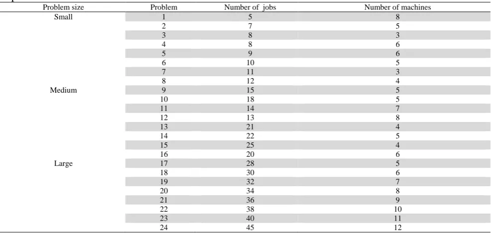
In order to evaluate the performance of the proposed metaheuristics, several computational experiments are presented. Since there is no benchmark for this problem, random instances are generated. The sequence dependent setup times are drawn from a uniform distribution over an interval [10,20] and the process times are uniformly drawn from the interval [30,50]. Learning parameter (α) distributes uniformly over interval [-0.4,0]. The examples are classified into 3 groups: small, medium and large instances. In each group eight problems are considered, in which Number of jobs and machines are different in each category. Table 3 shows details of each instance. In order to optimize the performance of proposed metaheuristics, GA and SA parameters were tuned. GA parameters which should be calibrated include population size (pop size), number of generations, the probability of crossover (𝑃𝑃𝑐𝑐), probability of mutation (𝑃𝑃𝑚𝑚) and elits rate (𝑃𝑃𝑟𝑟). On the other hand SA parameters consist of number of population (Npop) number of moves (Nmove) maximum iteration (Maxit) and the parameter which controls the cooling procedure (α). One of the best known ways for tunnig parameters is Taguchi method. In this paper, Minitab software is used to design the experiments and assign the best level for each size of problems. The Taguchi's prefered design for GA is 𝐿𝐿27(35) orthogonal array. This array is to deal with five parameters in three levels and the Taguchi's prefered design for SA is 𝐿𝐿9(34) orthogonal array which handles four parameters in three levels.
Table 3
Properties of instances
Problem size Problem Number of jobs Number of machines
Small 1 5 8
2 7 5
3 8 3
4 8 6
5 9 6
6 10 5
7 11 3
8 12 4
Medium 9 15 5
10 18 5
11 14 7
12 13 8
13 21 4
14 22 5
15 25 4
16 20 6
Large 17 28 5
18 30 6
19 32 7
20 34 8
21 36 9
22 38 10
23 40 11
24 45 12
1
i i
The examinations are conducted for each combination of factors. Parameter levels of both meta-heuristics and obtained results from Taguchi method are shown in Table 4 and Table 5. The proposed algorithms are coded in MATLAB (R2013a) and the proposed mathematical model is coded in GAMS-IDE optimization software. The experiments are performed on a PC with a 2.4 GHz Intel Core i5 processors and 6 GB of RAM memory.
In this paper, two performance criteria are measured. The first criterion is named relative percentage deviation (RPD). It is calculated using Eq. (19):
(19)
𝐿𝐿𝑃𝑃𝑆𝑆 =𝑎𝑎𝑎𝑎𝑎𝑎𝑎𝑎𝑎𝑎𝑖𝑖𝑠𝑠ℎ𝑚𝑚𝑠𝑠𝑠𝑠𝑠𝑠𝑠𝑠𝑠𝑠𝑖𝑖𝑠𝑠𝑛𝑛𝑚𝑚𝑖𝑖𝑛𝑛 − 𝑚𝑚𝑖𝑖𝑛𝑛𝑠𝑠𝑠𝑠𝑠𝑠𝑠𝑠𝑠𝑠𝑖𝑖𝑠𝑠𝑛𝑛
𝑠𝑠𝑠𝑠𝑠𝑠𝑠𝑠𝑖𝑖𝑠𝑠𝑛𝑛
The second one is an improvement factor surveying the algorithm performance and is calculated as Eq.
(20).
(20)
𝐼𝐼𝑚𝑚𝑝𝑝= 𝑎𝑎𝑎𝑎𝑎𝑎𝑎𝑎𝑎𝑎𝑖𝑖𝑠𝑠ℎ𝑚𝑚𝑖𝑖𝑛𝑛𝑖𝑖𝑠𝑠𝑖𝑖𝑖𝑖𝑠𝑠𝑠𝑠𝑠𝑠𝑠𝑠𝑠𝑠𝑖𝑖𝑠𝑠𝑛𝑛𝑎𝑎𝑎𝑎𝑎𝑎𝑎𝑎𝑎𝑎𝑖𝑖𝑠𝑠ℎ𝑚𝑚− 𝑎𝑎𝑎𝑎𝑎𝑎𝑎𝑎𝑎𝑎𝑖𝑖𝑠𝑠ℎ𝑚𝑚𝑓𝑓𝑖𝑖𝑛𝑛𝑖𝑖𝑠𝑠𝑠𝑠𝑠𝑠𝑠𝑠𝑠𝑠𝑠𝑠𝑖𝑖𝑠𝑠𝑛𝑛
𝑖𝑖𝑛𝑛𝑖𝑖𝑠𝑠𝑖𝑖𝑖𝑖𝑠𝑠𝑠𝑠𝑠𝑠𝑠𝑠𝑠𝑠𝑠𝑠𝑖𝑖𝑠𝑠𝑛𝑛
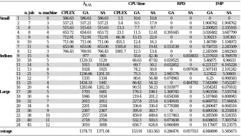
To minimize the errors, each problem is solved ten times by each procedure and mean of obtained results are shown in Table 6. Since the required time for solving the problems by the exact method increases exponentially, only small problems were solved by both CPLEX solver in GAMS and proposed metaheuristics. The medium and large instances were only solved by proposed metaheuristics. As shown in the Table 6, both GA and SA are capable of finding the best solutions for small problems. For medium problems, SA usually outperforms GA and in large size problems, SA has mostly a better function than GA. In order to evaluate the accuracy of obtained results, a 95% confidence interval graph of RPDs is shown in Fig. 1. It is clear that SA RPD is much less than GA RPD and the tolerance of upper and lower bounds in GA is more than SA. Thus, SA with a minimum lower and upper bound is better than GA and it can be concluded that the results obtained from SA algorithm is more reliable.
Table 4
GA parameters and levels
Lower limit(-) Upper limit (+)
Popsize generation 𝑃𝑃𝑐𝑐 𝑃𝑃𝑚𝑚 𝑃𝑃𝑟𝑟
(-) (+) (-) (+) (-) (+) (-) (+) (-) (+)
For small problems 100 200 80 120 0.6 0.8 0.1 0.2 0.3 0.7
Appropriate quantity 150 80 0.7 0.15 0.7
For medium problems 150 250 120 180 0.6 0.8 0.1 0.2 0.3 0.7
Appropriate quantity 250 180 0.6 0.2 0.7
For large problems 200 300 180 300 0.6 0.8 0.1 0.2 0.3 0.7
Appropriate quantity 250 300 0.6 0.2 0.7
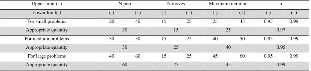
Table 5
SA parameters and levels
Upper limit (+) N.pop N.moves Maximum iteration α
Lower limit(-) (-) (+) (-) (+) (-) (+) (-) (+)
For small problems 20 40 15 25 25 45 0.95 0.99
Appropriate quantity 30 15 25 0.97
For medium problems 30 50 15 25 40 50 0.95 0.99
Appropriate quantity 30 25 40 0.95
For large problems 40 60 15 25 45 60 0.95 0.99
The improvement factor of meta-heuristics is compared in interval plot shown in Fig. 2. It can be inferred from this figure that, both GA and SA have appropriate ability of searching and improving the initial solutions. However, in this case, SA performs better.
Fig. 3 illustrates the difference between computational time of GA and SA for small instances. The figure shows that as the size of problems becomes larger the required times to solve the problem by exact method increase.
Table 6
Computation results obtained by the proposed algorithms and CPLEX based on problem type and dimensions
𝑪𝑪𝒎𝒎𝒎𝒎𝒎𝒎 CPU time RPD IMP
n. job n. machine CPLEX GA SA CPLEX GA SA GA SA GA SA
Small 1 5 8 586.63 586.63 586.63 1.5 10.6 10.8 0 0 0 0
2 7 3 537.21 537.21 537.21 5.4 9.5 17.9 0 0 1.904762 1.904762
3 8 5 515.63 515.63 515.63 13.3 7.7 9.7 0 0 2.200825 2.335165
4 8 4 653.72 654.63 653.72 23.1 11.5 12.41 0.391645 0 3.026482 3.647799
5 9 6 712.91 712.91 712.91 66.36 13.15 22.9 0 0 3.39213 3.91363
6 10 5 711.06 711.06 711.06 455.1 12.4 16.3 0 0 1.46789 1.104972
7 11 6 653.06 653.06 653.06 1505.8 10.5 19.41 0.153139 0 0.758725 2.245509
8 12 3 766.43 769.93 766.43 1881.7 12.5 13.4 0 0 2.245509 2.682563
Medium 9 15 6 977 985 55.6 42.36 0 0.818833 5.237633 4.769578
10 18 5 1129.33 1129 66.63 47.92 0.029525 0 5.46875 4.96633
11 14 5 1015 1014.66 69.7 50.2 0.032852 0 6.221127 6.165228
12 13 8 1024 1025 74.2 50.8 0 0.097656 2.507141 2.101242
13 21 5 1236.66 1201.33 75.3 55.3 2.941176 0 3.23422 5.50603
14 22 7 1335 1334 80.6 56.48 0.074963 0 6.25 6.908583
15 25 4 1434.33 1441 86.42 54.32 0 0.464792 7.541899 7.052247
16 20 4 1283.66 1282.33 90.51 58.23 0.103977 0 5.054241 6.079102
Large 17 28 5 1703 1681 176.5 198.1 1.308745 0 5.963556 7.535754
18 30 6 1846 1834 219.4 201.2 0.654308 0 5.187468 6.808943
19 32 7 2015 2012 227.8 215.8 0.149105 0 6.669755 17.94454
20 34 8 2201 2184 336.6 330.4 0.778388 0 6.260647 6.064516
21 36 9 2367 2367 395.9 383.7 0 0 8.680556 8.255814
22 38 10 2557 2554 459.9 449.6 0.117463 0 8.285509 8.524355
23 40 11 2718 2716 532.3 503.5 0.073638 0 8.638655 7.303754
24 45 12 3010 3008 658.7 624.8 0.066489 0 10.17607 10.23575
Average 1374.71 1371.04 153.91 143.563 0.286476 0.057553 4.848898 5.585673
The improvement factor of meta-heuristics is compared in interval plot shown in Fig. 2. It can be inferred from this figure that, both GA and SA have appropriate ability of searching and improving the initial solutions. However, in this case, SA performs better.
Fig. 3 illustrates the difference between computational time of GA and SA in small instances. The figure shows that as the problems become larger the required times to solve the problem by exact method increase.
R
PD
SA GA
0.6 0.5 0.4 0.3 0.2 0.1 0.0
Inte rval Plot of GA; SA 95% CI for the Mean
IM
P
SA GA
7.5 7.0 6.5 6.0 5.5 5.0 4.5 4.0 3.5
Inte rval Plot of GA; SA 95% CI for the Mean
Fig. 2. Mean and interval plot for the RPD of GA and SA
So for real-world problems CPLEX solver of GAMS is not practical. Moreover, in most instances GA needs less time to reach to optimal solution.
In Fig. 4, the required CPU times for solving medium problems are shown. As it is shown SA performs faster and converges to optimal solution in less time.
Fig. 4. Comparison of computational time of the GAMS, GA and SA in small problems
Fig. 5. Comparison of computational time of the GA and SA in medium problems
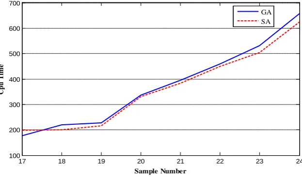
In Fig. 5, computational times of SA and GA for large size problems are compared. In most cases the difference is negligible, but SA has better performance in comparison with GA.
Fig. 6. Comparison of computational time of the GA and SA in large size problems 6. Conclusion
This paper dealt with the “m-machine no-wait flowshop scheduling” problem to minimize makespan with respect to sequence-dependent setup times and truncated learning function. In most researches learning effect was only considered in job times and it is the same for every job. Also a few studies have considered learning effect in m-machine flowshop. However, in this paper learning effect is applied to set up times and learning factors differ from one machine to another one. This problem is modeled using a mixed-integer linear programming. Three-machine no-wait flowshop has been proved NP-complete; therefore, this problem, considering more complex restrictions, is also NP-hard so exact methods are not suitable to solve this problem in large scale instances. Therefore, an improved Genetic algorithm and a Simulated Annealing are proposed to solve random sample problems. The answers were analyzed using three main criteria. Computational experiments have shown that both proposed meta-heuristics are powerful to solve the problems within reasonable computation time. Nonetheless, with respect to the computational results in this problems, SA has better performance than GA.
0 1 2 3 4 5 6 7 8
100 101 102 103 104
Sample Number
C
pu T
im
e
GAMS GA SA
9 10 11 12 13 14 15 16
40 50 60 70 80 90 100
Sample Number
C
pu T
im
e
GA SA
17 18 19 20 21 22 23 24
100 200 300 400 500 600 700
Sample Number
C
pu T
im
e
References
Allahverdi, A., & Aldowaisan, T. (2001). Minimizing total completion time in a no-wait flowshop with sequence-dependent additive changeover times. Journal of the Operational Research Society, 52(4), 449-462.
Allahverdi, A., & Aydilek, H. (2014). Total completion time with makespan constraint in no-wait flowshops with setup times. European Journal of Operational Research, 238(3), 724-734.
Allahverdi, A., & Aldowaisan, T. (2002). No-wait flowshops with bicriteria of makespan and total completion time. Journal of the Operational Research Society, 53(9),1004-1015.
Ben Chihaoui, F., Kacem, I., Hadj-Alouane, A. B., Dridi, N., & Rezg, N. (2011). No-wait scheduling of a two-machine flow-shop to minimise the makespan under non-availability constraints and different release dates. International Journal of Production Research, 49(21), 6273-6286.
Biskup, D. (1999). Single-machine scheduling with learning considerations. European Journal of
Operational Research, 115(1), 173-178.
Biskup, D. (2008). A state-of-the-art review on scheduling with learning effects. European Journal of
Operational Research, 188(2), 315-329.
Chen, P., Wu, C. C., & Lee, W. C. (2006). A bi-criteria two-machine flowshop scheduling problem with a learning effect. Journal of the Operational Research Society, 57(9), 1113-1125.
Cheng, T. C. E., Wu, C. C., Chen, J. C., Wu, W. H., & Cheng, S. R. (2013). Two-machine flowshop scheduling with a truncated learning function to minimize the makespan. International Journal of
Production Economics, 141(1), 79-86.
Cheng, T. E., & Wang, G. (2000). Single machine scheduling with learning effect considerations. Annals
of Operations Research, 98(1-4), 273-290.
Ding, J. Y., Song, S., Gupta, J. N., Zhang, R., Chiong, R., & Wu, C. (2015). An improved iterated greedy algorithm with a Tabu-based reconstruction strategy for the no-wait flowshop scheduling problem.
Applied Soft Computing, 30, 604-613.
Eren, T., & Güner, E. (2008). A bicriteria flowshop scheduling with a learning effect. Applied
Mathematical Modelling, 32(9), 1719-1733.
Goldberg, D. E., & Holland, J. H. (1988). Genetic algorithms and machine learning. Machine learning,
3(2), 95-99.
İşler, M. C., Toklu, B., & Çelik, V. (2012). Scheduling in a two-machine flow-shop for earliness/tardiness under learning effect. The International Journal of Advanced Manufacturing Technology, 61(9-12), 1129-1137.
Janiak, A., Janiak, W. A., Rudek, R., & Wielgus, A. (2009). Solution algorithms for the makespan minimization problem with the general learning model. Computers & Industrial Engineering, 56(4), 1301-1308.
Kirkpatrick, S., & Vecchi, M. P. (1983). Optimization by simmulated annealing. Science, 220(4598), 671-680.
Lai, K., Hsu, P. H., Ting, P. H., & Wu, C. C. (2014). A Truncated Sum of Processing‐Times–Based Learning Model for a Two‐Machine Flowshop Scheduling Problem. Human Factors and Ergonomics
in Manufacturing & Service Industries, 24(2), 152-160.
Lee, W. C., & Wu, C. C. (2004). Minimizing total completion time in a two-machine flowshop with a learning effect. International Journal of Production Economics, 88(1), 85-93.
Lee, W. C., & Wu, C. C. (2009). Some single-machine and m-machine flowshop scheduling problems with learning considerations. Information Sciences, 179(22), 3885-3892.
Li, D. C., Hsu, P. H., Wu, C. C., & Cheng, T. E. (2011). Two-machine flowshop scheduling with truncated learning to minimize the total completion time. Computers & Industrial Engineering, 61(3), 655-662.
Liu, Y., & Feng, Z. (2014). Two-machine no-wait flowshop scheduling with learning effect and convex resource-dependent processing times. Computers & Industrial Engineering, 75, 170-175.
Murata, T., Ishibuchi, H., & Tanaka, H. (1996). Genetic algorithms for flowshop scheduling problems.
Nagano, M. S., & Araújo, D. C. (2014). New heuristics for the no-wait flowshop with sequence-dependent setup times problem. Journal of the Brazilian Society of Mechanical Sciences and
Engineering, 36(1), 139-151.
Nagano, M. S., Da Silva, A. A., & Lorena, L. A. N. (2014). An evolutionary clustering search for the no-wait flow shop problem with sequence dependent setup times. Expert Systems with Applications,
41(8), 3628-3633.
Röck, H. (1984). The three-machine no-wait flowshop is NP-complete. Journal of the ACM (JACM),
31(2), 336-345.
Samarghandi, H., & ElMekkawy, T. Y. (2014). Solving the no-wait flow-shop problem with sequence-dependent set-up times. International Journal of Computer Integrated Manufacturing, 27(3), 213-228.
Shiau, Y. R., Tsai, M. S., Lee, W. C., & Cheng, T. C. E. (2015). Two-agent two-machine flowshop scheduling with learning effects to minimize the total completion time. Computers & Industrial
Engineering, 87, 580-589.
Wang, J. B., & Liu, L. L. (2009). Two-machine flowshop problem with effects of deterioration and learning. Computers & Industrial Engineering, 57(3), 1114-1121.
Wang, J. B., & Wang, J. J. (2014). Flowshop scheduling with a general exponential learning effect.
Computers & Operations Research, 43, 292-308.
Wang, J. B., & Xia, Z. Q. (2005). Flow-shop scheduling with a learning effect. Journal of the Operational
Research Society, 56(11), 1325-1330.
Wang, J. J., & Zhang, B. H. (2015). Permutation flowshop problems with bi-criterion makespan and total completion time objective and position-weighted learning effects. Computers & Operations Research,
58, 24-31.
Wu, C. C., Lee, W. C., & Wang, W. C. (2007). A two-machine flowshop maximum tardiness scheduling problem with a learning effect. The International Journal of Advanced Manufacturing Technology,
31(7-8), 743-750.
Wu, Y. B., & Wang, J. J. (2015). Single-machine scheduling with truncated sum-of-processing-times-based learning effect including proportional delivery times. Neural Computing and Applications, 1-7. Wu, W. H., Wu, W. H., Chen, J. C., Lin, W. C., Wu, J., & Wu, C. C. (2015). A heuristic-based genetic algorithm for the two-machine flowshop scheduling with learning consideration. Journal of
Manufacturing Systems, 35, 223-233.
Ying, K. C., Lee, Z. J., Lu, C. C., & Lin, S. W. (2012). Metaheuristics for scheduling a no-wait flowshop manufacturing cell with sequence-dependent family setups. The International Journal of Advanced
Manufacturing Technology, 58(5-8), 671-682.