www.clim-past.net/6/827/2010/ doi:10.5194/cp-6-827-2010
© Author(s) 2010. CC Attribution 3.0 License.
Climate
of the Past
A multi-variable box model approach to the soft tissue carbon pump
A. M. de Boer1, A. J. Watson1, N. R. Edwards2, and K. I. C. Oliver3
1School of Environmental Science, University of East Anglia, Norwich, NR4 7TJ, UK
2Earth and Environmental Sciences, Open University, Walton Hall, Milton Keynes, MK7 6AA, UK
3School of Ocean and Earth Science, National Oceanography Centre, Southampton, University of Southampton,
Southampton, SO14 3ZH, UK
Received: 29 April 2010 – Published in Clim. Past Discuss.: 17 May 2010
Revised: 17 October 2010 – Accepted: 28 November 2010 – Published: 21 December 2010
Abstract. The canonical question of which physical, chem-ical or biologchem-ical mechanisms were responsible for oceanic uptake of atmospheric CO2during the last glacial is yet
unan-swered. Insight from paleo-proxies has led to a multitude of hypotheses but none so far have been convincingly supported in three dimensional numerical modelling experiments. The processes that influence the CO2uptake and export
produc-tion are inter-related and too complex to solve conceptually while complex numerical models are time consuming and expensive to run which severely limits the combinations of mechanisms that can be explored. Instead, an intermedi-ate inverse box model approach of the soft tissue pump is used here in which the whole parameter space is explored. The glacial circulation and biological production states are derived from these using proxies of glacial export produc-tion and the need to draw down CO2 into the ocean. We
find that circulation patterns which explain glacial observa-tions include reduced Antarctic Bottom Water formation and high latitude upwelling and mixing of deep water and to a lesser extent reduced equatorial upwelling. The proposed mechanism of CO2 uptake by an increase of eddies in the
Southern Ocean, leading to a reduced residual circulation, is not supported. Regarding biological mechanisms, an in-crease in the nutrient utilization in either the equatorial re-gions or the northern polar latitudes can reduce atmospheric CO2and satisfy proxies of glacial export production.
Consis-tent with previous studies, CO2is drawn down more easily
through increased productivity in the Antarctic region than the sub-Antarctic, but that violates observations of lower ex-port production there. The glacial states are more sensitive to changes in the circulation and less sensitive to changes in nutrient utilization rates than the interglacial states.
Correspondence to: A. M. de Boer ([email protected])
1 Introduction
During the last 800 000 years atmospheric pCO2 has
var-ied in concert with Antarctic surface air temperature (EPICA Community Members, 2004; L¨uthi et al., 2008; Petit et al., 1999; Siegenthaler et al., 2005). Determining the mecha-nisms behind the correlation remains a tantalizing question in paleoclimatology today. Kohfeld and Ridgwel (2009) pro-vide an excellent review of the processes that are known or proposed to play an important role in lowering glacial atmo-sphericpCO2. They conclude from previous work that lower
sea surface temperatures can explain approximately 26 ppmv (21–30 ppmv) of the interglacial to glacialpCO2 decrease
and that this decrease was countered by a reduction in the terrestrial biosphere and reduced ice volume which resulted in an increase of about 22 ppmv (12–36 ppmv) and 13 ppmv (11–17 ppmv) respectively. Other lesser understood mech-anisms include changes in the ocean circulation, aeolian Fe fertilization, bacterial metabolic rate change, Si fertilization, and coral reef growth.
The observedpCO2-temperature correlation in the glacial
record is much stronger in the Antarctic (AA) than in the Northern hemisphere Greenland records. This is partly be-cause of the more complex and variable atmospheric circula-tion patterns that prevail over Greenland. However, the very good correspondence of temperature andpCO2 in
Antarc-tica suggest that the Southern Ocean (SO) played an impor-tant role in the glacial carbon cycle. Oceanic uptake of atmo-spheric CO2through air sea gas exchange is facilitated by the
The zonally integrated transport in the SO can be divided into a deep poleward cell of which the downwelling branch represents Antarctic Bottom Water (AABW) formation and an upper, more equatorward cell referred to as the SO resid-ual circulation (Karsten and Marshall, 2002; Marshall and Radko, 2003). Increased net uptake of atmospheric CO2
(through reduced outgassing of CO2) has been proposed to
be a result of a weakening of the poleward cell though en-hanced surface stratification or reduced winds (Sigman and Boyle, 2001; Sigman et al., 2004; Toggweiler et al., 2006; Francois et al., 1997) or a weakening of the residual cir-culation through reduced buoyancy or winds (Watson and Garabato, 2006; Fischer et al., 2010; Parekh et al., 2006). A reduction in either of these cells would imply less deep upwelling during the glacial for which evidence remains am-biguous (Anderson et al., 2009; De Pol-Holz et al., 2010). As noted, given a steady state circulation, the atmospheric CO2
can also be reduced through increased biological production in the SO (Sarmiento and Toggweiler, 1984). The main hy-pothesis for lowering glacialpCO2as a consequence of
in-creased SO biological export is that there was an enhanced supply of the limiting micro nutrient iron (Martin, 1990; Joos et al., 1991; Watson et al., 2000; Parekh et al., 2008; Brovkin et al., 2007).
The role of the equatorial upwelling regions in the carbon cycle is still under debate. Matsumoto and Sarmiento (2002) suggested that, during the last glacial, smaller Si:N ratios in Antarctic plankton led to more Si leakage to equatorial re-gions where higher Si enhanced diatom production (at the expense of cocolithophores) weakened the carbonate pump. Sediment core data does not reveal the high opal fluxes needed to support the Si leakage hypothesis (Bradtmiller et al., 2006) but Pichevin et al. (2009) recently argued that the lower equatorial opal burial rate is due to a decrease in the silicon to carbon uptake ratio found in iron rich environ-ments. The hypothesis is supported by clear evidence for an enhanced glacial iron supply to the Eastern Equatorial Pa-cific (McGee et al., 2007; Winckler et al., 2008). It should be noted that more organic matter export from the Equato-rial Pacific does not necessarily imply a stronger soft tissue pump. Enhanced equatorial nutrient utilization could also imply a geographical shift in global export production (i.e., from the sub-tropics to the tropics) rather than an overall in-crease.
The traditional process through which solutions to the glacial carbon problem are sought can, conceptually at least, be seen as comprising of four steps. The first step is to mea-sure or assimilate existing knowledge of the glacial state (i.e., proxies of the atmospheric and oceanic biochemistry and cir-culation). The second step is to form a hypothesis of a spe-cific mechanism that may have led to a glacial atmospheric drawdown of CO2. As a next step, the hypothesis is often
tested in a simple box model in which the general circula-tion is set as close as possible to observacircula-tions and the sensi-tivity of the atmospheric pCO2 to the specific mechanism
is derived. If the result is promising, the final step is to verify the hypothesis in a more complex ocean or coupled model. Ideally not only the CO2uptake, but also the
circu-lation and biology of the glacial simucircu-lation should be con-sistent with the observations in step one. All four of these steps are needed and each step has obvious advantages and drawbacks. The main problem with the box model approach is that it requires the simplification of the circulation and bi-ology in ways that are rather ad hoc and the implications of these simplifications for the conclusions are not clear. The physical and biological processes in general circulation mod-els are closer to that of the real world. However, they are expensive to run and, perhaps more importantly, it is often impossible to distinguish in a complex model between var-ious mechanisms for CO2uptake. For example, increasing
the SO winds stress has an effect on the AABW formation, sea ice, the residual circulation and the North Atlantic deep water formation and it is therefore not clear how the resulting atmospheric CO2concentration has come about.
We propose here a new type of box model that eliminates some of the common problems with box models associated with hidden sensitivities to input parameters. It is inexpen-sive to run so that all combinations of circulation and bio-logical CO2uptake mechanisms can be explored in
conjunc-tion with each other or in isolaconjunc-tion. It is akin to an inverse model in that we deduce the circulation and biological pa-rameters for the interglacial and glacial from observations rather than assume any values a priori. The primary obser-vations used to determine the interglacial states are observed phosphate distributions. For the glacial we isolate states that draw down the most CO2and whose export production in
re-lation to the interglacial is consistent with the observational synthesis of Kohfeld et al. (2005). The bulk of the evidence suggests decreased export in the Antarctic region of the SO, and increased export in the Sub-Antarctic and the Equatorial upwelling regions. Because all our input parameters assume the whole range of realistic values, there are no hidden sensi-tivities other than those built into the geometry of the model. We explore two other model setups to ensure that our con-clusions are not highly dependent on the geometry.
The purpose of this study is to identify which types of glacial circulation and productivity regimes are consistent with the observations and to relate these to current hypothe-ses for glacial oceanic uptake of atmospheric CO2. A
de-tailed description of the model is provided in the next section as well as the link between preformed nutrient concentration and atmosphericpCO2. In Sect. 3 we present the most likely
solutions of the glacial and interglacial, and explore the sen-sitivity of thepCO2and export production to the circulation
2 Methods
2.1 Model description
Our standard model has seven boxes of which six are in the upper 500 m (Fig. 1a). As is typical in box models (Wat-son and Garabato, 2006; John(Wat-son et al., 2007), we assume a closed system that represents a zonally integrated ocean. Combining the Atlantic and Indo-Pacific into one basin is not ideal but the assumptions we shall make about latitudi-nal distributions of nutrients and export and where water up-wells and sinks, hold in both basins. The SO is divided into an Antarctic box and a sub-Antarctic box and the division is roughly at the polar front, assumed to be at 55◦S. The low latitudes extend from 40◦S to 40◦N and are intersected by a narrow box, from 10◦S to 10◦N, which explicitly represents the high nutrient equatorial upwelling region. A northern box starts at 40◦N and extends to the north pole. The volumes of the surface boxes are the same as in the real world between these specified zonal boundaries and for the deep box be-tween 500 m and the bottom. We shall use the term SO to describe both the Antarctic and the Sub-Antarctic boxes. In order to relate the model to the real world, we refer to the sinking in the Antarctic box as AABW.
The fluxes between the boxes are fully described by five independent model parameters: (1) Antarctic deep water for-mation,TA, (2) northward surface Ekman transport between
the two SO surface boxes, TT, (3) a southward transport
representing the contribution of SO mesoscale eddies,TME,
(4) an equatorial upwelling flux,TEU, and (5) a northern
up-welling flux,TNU. These variables are indicated in Fig. 1a
and the range of values they take is listed in Table 1. The rest of the transport terms are quantities derived from conti-nuity. Note that the southward eddy flux is never more than the northward Ekman transport so that the residual flow into the equatorial box is always positive. Upwelling in the SO occurs in the Antarctic box (south of the polar front) and is equal to the net flow out of the box from Antarctic sink-ing and the residual circulation. In the northern box the up-welling is balanced by local downup-welling so that it can be seen as a mixing term that brings up high nutrient water to the surface similar to winter mixing in the real ocean. The upwelling in the equatorial box represents both wind driven upwelling and that due to turbulent mixing. There is no sim-ple way to represent the comsim-plex dynamics of the equatorial region – we have chosen to return the upwelled water to the deep ocean in the northern box but in reality some downward mixing of the surface properties occurs locally and some of the upwelled water is subducted in the low latitudes. To en-sure that our results are not highly dependent on equatorial upwelling or the northern sinking that goes along with it, the study is repeated in a model that does not have an equato-rial box (Fig. 1b). In this case the equatoequato-rial box is treated the same way as the low latitude boxes. In another test of
Fig. 1. The control model consists of 7 upper boxes above 500m
and one deep box (a). Export production is denoted by the dotted arrows and is the product of the nutrients concentration and a nu-trient utilization rate that varies for each surface box (see text for details). The flow of water between the boxes has five dimensions of freedom and we have labelled the flux as they are used in the equations and figures. The unlabeled fluxes are derived from the prescribed fluxes and conservation of mass. A second model is pre-sented in which the equatorial region has been integrated into the low latitude boxes (b).
the effect of the geometry the upper layer depth was reduced from 500 m to 300 m.
The soft tissue biological pump in our model is simplified to a one-nutrient formulation,P, denoting phosphate (PO4).
The nutrients are advected by the circulation in the usual way. Export production from a surface box is linearly proportional to the nutrient concentration in the box. The proportionality constant,α, differs from box to box and encapsulates factors which limit the uptake of nutrients such as light or iron. It is referred to in the rest of the text as the nutrient utilization rate and is the fraction of the available nutrients that is exported from the surface as organic matter (rather than as preformed nutrients) each second. This constant is allowed to vary over a wide range of values (Table 1). The export production from the box is then simply,αP, multiplied by the volume of the box. The overall nutrient content is set to be the same as that derived from the World Ocean Atlas of 2005 (Garcia et al., 2006). The above model is mathematically formulated in the following seven equations,
Box A: TAUPD−(TA+TT+αAVA) PA+TMEPS =0
Box S: TTPA − (TT +αSVS) PS = 0
Table 1. Model parameters for the standard 7 box model. For each box the volume and the observed PO4concentrations for the real ocean between the same boundaries (derived from the World Ocean Atlas 2006) is given. The range of nutrient utilization rates for each box and transport fluxes between the boxes indicate the parameter space that is covered by the 107solutions.
Model Box Volume Observed PO4 Nutrient utilization,α
(1015m3) (10−6µmol kg−1) (10−10s−1)
Antarctic (A) 16 2.45 0–10
Sub-A (S) 21 1.70 0–10
Lowlat-south (LS) 47 1.04 0–10
Equator (E) 32 1.89 0–10
Low lat-north (LN) 36 1.23 0–10
North (N) 16 1.60 0–10
Deep Ocean (D) 1300 2.64
Transport Flux Transport
(106m3s−1)
AABW (TAU) 0–20
Ekman (TT) 0–30
SO eddies (TME) 0–30
EQ upwelling (TE) 0–20
Northern upwelling (TNU) 0–20
Box E: TEUPD + (TT −TME) PLS
−(TT −TME +TEU +αEVE) PE = 0
Box LN:(TT −TME + TEU) PE
−(TT −TME +TEU +αLNVLN) PS = 0
Box N: TNUPD + (TT −TME +TEU) PLN
−(TT−TME+TEU+TNU+αNVN) PN = 0
All: VDPD +VAPA +VLSPLS +VSPS +VEPE +VLNPLN +VNPN = PSUM,
whereT is a transport variable andV the box volume. The subscripts A, S, LS, E, LN, N, and D denote the Antarctic box, Sub-Antarctic box, Low latitude Southern box, Equa-torial box, Low Latitude Northern box, Northern box, and Deep box respectively. Upwelling fluxes into the boxes have a U at the end, i.e., TAUis upwelling into the Antarctic box.
The SO Ekman transport and mesoscale eddy transport are denoted byTT andTME respectively andPSUM is the total
amount of PO4molecules in the ocean. These equations are
solved for 107 random combinations of the five circulation and five nutrient utilization input parameters (see Table 1 for range). Note that the six surface boxes give only five nutrient utilization parameters because we assume that the conditions for biological production in the northern and southern low latitude regions are similar and therefore setαto be the same in these boxes (i.e.,αLS=αLN).
2.2 The relation of preformed nutrients to atmospheric CO2
During glacial periods CO2is drawn into the ocean through
an increase in the surface to deep gradient of dissolved in-organic carbon (DIC). This gradient relies on the soft tissue biological pump in which carbon is being sequestrated into organic matter in the surface and later remineralized in the deep ocean. Nutrients that are advected to the deep ocean as a result of the physical circulation of the ocean are not avail-able for biological uptake and are referred to as preformed nutrients. If the proportion of preformed nutrients in the deep ocean is large, the biological pump is inefficient, the vertical gradient of DIC weak, and the atmospheric CO2high. The
strong positive relation between preformed nutrients and at-mospheric CO2has been derived theoretically (Ito and
Fol-lows, 2005; Goodwin et al., 2008) and confirmed in ocean general circulation models (Ito and Follows, 2005; Marinov et al., 2006). In our model we describe the biology in terms of the macro nutrient PO4and then we use this theory (Ito
and Follows, 2005) to relate the preformed nutrient concen-tration to atmospheric CO2. For completeness and to alert
the reader of the assumptions made, we briefly summarise the theory here. For a more comprehensive derivation please refer to the original reference.
Dissolved inorganic carbon in the ocean can be subdivided into preformed and regenerated carbon. The preformed con-centration can in turn be written as the sum of a saturated component Csat and a preindustrial air-sea disequilibrium
Ccalcite. Assuming a constant reservoir of carbon in the ocean
and atmosphere, a small change in thepCO2 of the
atmo-sphere can be written in terms of the changes in the oceanic carbon components, i.e.,
Mδ pCOatm2 +VδCsat+δ1 C+δCorg+δCcalcite =0 (1)
whereMis the total moles of gas in the atmosphere andV is the volume of the ocean. For simplicity it is assumed that changes in the soft tissue pump are independent of changes in the carbonate pump or saturation so thatδ1C=δCcalcite=
0). Using the Buffer factor,B(Bolin and Erikson, 1959), one can approximate variations inδ Csatby
δlnpCOatm2 = B δlnCsat (2)
EliminatingCsatfrom Eqs. (1) and (2) gives an expression
for the sensitivity ofpCOatm2 toCorg
δpCOatm2 δ Corg
= V
M γ (3)
where
γ ≡ 1 + V Csat
B M pCOatm2 (4)
We now define the efficiency of the biological pump, P∗ ≡ Preg
P0
(5) wherePregis the mean regenerated phosphate concentration
andP0 is the global mean phosphate concentration. For a
100% efficient pump P∗ will be 1. A perturbation in the organic carbon concentration can be written in terms of an equivalent change in the biological pump using a fixed Red-field ratio,
δCorg = RC:P δPreg = RC:P P0δP∗ (6)
Combining Eqs. (3), (4) and (6), a linear relation between pCOatm2 and the efficiency of the biological pump as defined by Eq. (5) is found,
δpCOatm2 δP∗
= V RC:P P0
M γ ∼ 312 ppmv (7)
In our model, the preformed nutrient concentration is defined as the fraction of nutrients that reach the deep ocean through the circulation multiplied by the deep ocean nutrient concen-tration. The biological pump efficiency is the fraction of nu-trients that is exported to the deep ocean through biological productivity and ranges from near 0 to 100% for our 107 so-lutions (Fig. 2). The preformed nutrient concentration ranges from 0 - 2.5µmol Kg−1and can be related by Eq. (7) to a 1pCO2 of approximately 300. Given that the theory that
relates1pCOatm2 to a change in preformed nutrients concen-tration is not designed for large perturbations the results that pertain to large glacial-interglacial changes should be inter-preted with caution.
Fig. 2. Changes in the atmospheric CO2in the model as a func-tion of the preformed nutrients for all 107solutions (left axis) as calculated according to the theory of Ito and Follows (2005). A zero1pCO2is assumed at the average preformed nutrient concen-tration of our 300 best interglacial solutions (see Sect. 3.2 for an explanation of how these are derived). The1pCO2and preformed nutrients are also linearly related to the efficiency of the biological pump (right axis).
3 Results
3.1 The interglacial states
It is common in carbon cycle box models to set the circu-lation as close as possible to observations or model output or to tune it to give realistic solutions (Keir, 1988; Tog-gweiler, 1999; Watson and Garabato, 2006). While these approaches have merit, it is not clear to which extent the conclusions of the studies depend on the chosen circulation states. In this study the whole parameter range is explored to ensure that our conclusions are not dependant on a cho-sen parameter. Initially 107random solutions are calculated to cover all parameter combinations within the limitations of our model setup. From these we select the modern states according to the circulation and nutrient and organic matter export distributions. In the first step, solutions are required to have higher export in the Sub-Antarctic than in the Antarc-tic box, and higher export in the equatorial box, northern and sub-Antarctic boxes than in the low latitude boxes. The circulation of the modern state is required to have at least 20 Sv (1 Sv = 106m3s−1) of northward Ekman transport and AABW formation between 5 and 25 Sv (Table 2). Of the solutions that fulfil these criteria we consider the 300 solu-tions that best fit the modern phosphate distribution as de-rived from the World Ocean Atlas 2005 (Garcia et al., 2006). The maximum deviation from PO4observations for any box
of any of the 300 solutions is 0.3 µmol kg−1).
Fig. 3. The circulation (top) and nutrient utilization rate (bottom)
parameters of the interglacial states (right) and the glacial states (left) are shown here against the preformed nutrient concentration in the deep ocean. The top axis relates the difference in preformed nutrient between the glacial and interglacial states to changes in at-mosphericpCO2(as discussed in Sect. 2.2). Best fit lines are drawn through the solutions for visual aid. They do not imply an indepen-dent linear correlation between the preformed nutrient concentra-tions and the input parameters.
sets. In this sense we effectively allow for model structural error using the plausibility approach of Holden et al. (2009) or Edwards et al. (2010). The Ekman transport and AABW cover the whole range of permitted values in the 300 solu-tions. To satisfy the observations of high surface nutrients, the northern and equatorial upwelling fluxes are towards the higher range of their permitted values. The eddy mass flux is somewhat on the low side so that the average residual circu-lation of the interglacial parameter sets is about 16 Sv, with a minimum of 4 Sv. The interglacial nutrient utilization rates have more confined patterns than the circulation parameters. Low utilization rates in the AA box, the low latitudes, and the equatorial box are necessary to simulate modern phos-phate distributions (Fig. 3, bottom right). The wide range of parameters that fulfil the basic interglacial criteria suggest that the traditional approach of picking one best guess state on which to do a sensitivity analysis may be unwise. The conclusions drawn in this study are instead based on all these states.
The purpose of isolating the best modern states is not to determine the real modern circulation or nutrient utilization. Rather, the modern states are obtained to (1) confirm that the model can reproduce a realistic interglacial state, (2) indicate the sensitivity ofpCO2 and nutrient concentrations to the
input parameters, given a modern state, and (3) provide ref-erence states with which to compare the glacial states. The
Table 2. Constraints used to derive the 300 interglacial and glacial.
EZdenotes the export flux from box Z and is equal toPZ·αz·VZ. The operator ()i indicates an average of the 300 interglacial states.
Period Essential constraint Final constraint
Interglacial TT>20 Sv The 300 states, fulfilling the 5 Sv< TA<25 Sv essential constraints, whose
EE> ELN,ELS PO4concentration most
ES> EA,ELS closely resemble the
ELN< EN observations as listed in Table 1.
Glacial EE>1.2 (EE)i The 300 states, fulfilling the
ES>1.2 (ES)i essential constraints, with
EA<0.8 (EA)i the lowest preformed nutrient concentration.
average efficiency of the biological pump of the 300 inter-glacial solutions is 35±4% which corresponds well with the estimate of 36% from Ito and Follows (2005).
3.2 The glacial states
Observations of the glacial ocean circulation are ambiguous but it is clear that the deep oceans were filled with a southern source water to a more shallow depth than today, and pore fluid measurements suggest this southern source water was much saltier than that from the North Atlantic (Ninnemann and Charles, 2002; Adkins et al., 2002b). Proxies for export production indicate increased export in the Sub-Antarctic and Equatorial regions and reduced export in the Antarctic region (Kohfeld et al., 2005). It is uncertain by how much the export has changed in each region – to select our most likely glacial states, we limited the solutions to those that have at least a 20% increase in export in the Sub-Antarctic and Equatorial boxes and a 20% decrease in the Antarctic box (Table 2). The resulting states are only weakly depen-dent on this number (i.e., the percentage rate). From these we select the 300 that have the lowest preformed nutrients, i.e., the states that are associated with the greatest draw down of CO2(Fig. 3, left). The average preformed nutrient
concentra-tion, biological pump efficiency, andpCO2change for these
states are 1.6 µmol kg−1, 84%, and−165 ppmv respectively. We choose the 300 states with the most severe drawdown of CO2as it illuminates clearly the parameters that are
impor-tant for CO2 uptake through the soft tissue pump, but our
conclusions are qualitative and hold also for smaller changes inpCO2, say or the order of−100 ppmv (confirmed, but not
shown).
Table 3. The mean and standard deviation of the change inpCO2due to a change in the input parameters for the 300 glacial and interglacial states, and for 300 randomly chosen states. For the circulation parameter the difference inpCO2due to a change in the circulation from 5 to 20 Sv is shown and for the nutrient utilization the difference inpCO2due to a change inαfrom 2 to 8e–10 s−1.
Transport fluxes Glacial Interglacial Random
(ppm/15 Sv) (ppm/15 Sv) (ppm/15 Sv)
AABW (TA) 73±6 26±5 44±20
Ekman (TT) 5±12 0±5 −7±16
Eddies (TME) −10±8 11±4 0±12
Eq-upwell (TE) 30±8 16±6 4±20
North-upwell (TN) 67±7 25±4 52±18
Model Boxes Glacial Interglacial Random
(ppm/6×1010s−1) (ppm/6×1010s−1) (ppm/6×1010s−1)
Antarctic (A) −5±2 −20±3 −20±10
Sub-Antarctic (S) −6±3 −16±3 −7±5
Low lats (LS, LN)) −27±7 −34±6 −19±12
Equatorial (E) −17±4 −28±4 −14±10
Northern (N) −14±4 −33±4 −31±13
on average 24 Sv. Interestingly, the southward eddy flux is never more than 20 Sv and always at least 9 Sv less than the Ekman transport (see Sect. 4.3 for discussion). Equatorial upwelling can take on any value in the glacial. The nutri-ent utilization rates in the low latitudes and northern boxes are not tightly constrained in the glacial states. However, the Antarctic nutrient utilization rate is always low and the Equatorial and Sub-Antarctic utilization rates are high. The implications of the results are discussed in Sect. 4. Note that the average change can be viewed as the most likely change and the range gives the possible solutions that are consistent with the observations.
The glacial and interglacial states have so far been pre-sented in terms of the input parameters and the preformed nu-trients. The actual variables that are solved for are the phos-phate concentrations. The average nutrient distribution for the 300 glacial states has a similar pattern to the interglacial although surface nutrients are reduced everywhere north of 40◦S (Fig. 4, top). The export production is higher by de-sign in the Equatorial and Sub-Antarctic boxes and lower in the Antarctic box of our modelled glacial states (Fig. 4, bot-tom). In the low latitude boxes we also find increased export which is consistent with the observations but this may well be fortuitous because the observations are in upwelling regions which we do not resolve in the model. The glacial states have a lower export production in the Northern box which is again consistent with the few data points north of 50◦N in the Kohfeld et al. (2005) reconstruction.
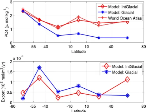
Fig. 4. The average surface nutrient concentrations (top) for the 300 interglacial states (solid red lines and diamonds) and the 300 glacial states (solid blue lines and stars). Also shown for refer-ence is the observed modern nutrient distribution (dashed red lines and crosses). Export production (bottom) from each surface box for the interglacial and glacial states. The modern nutrient distribution were obtained from the World Ocean Atlas (Garcia et al., 2006).
3.3 Sensitivity of preformed nutrients to circulation and nutrient utilization
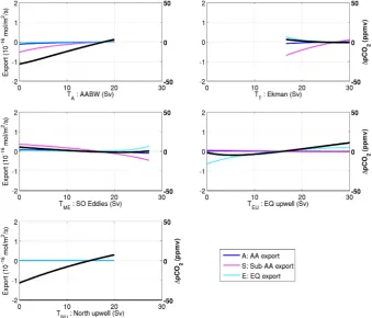
Fig. 5. The response of atmospheric1pCO2(solid black), Antarctic export production (from box A, solid dark blue), Sub-Antarctic export production (from box S, dashed magneta), and Equatorial export production (from box E, dashed light blue) to the five circulation input parameters,TA,TT,TME,TEU, andTNU. The export fluxes (left axis) and1pCO2(right axis) are expressed as the difference from that of the best fit interglacial change.
rates are that we need to look for in mechanisms to explain the glacial carbon cycle. It does not illustrate which of these parameters are responsible for the CO2drawdown and which
are only necessary to explain the proxy data of export pro-duction. For instance, it is likely that the reduced nutrient utilization rate in the glacial in the Antarctic box (Fig. 3) is necessary to reduce export there (as forced by the obser-vational constraint) and not to reduce preformed nutrients. Here we look at the sensitivity of thepCO2 and the export
production to the input parameters of the best fit interglacial state (Figs. 5 and 6). The export flux andpCO2are expressed
as the difference from the export andpCO2of the interglacial
state.
The sensitivities to input parameters are dependent on the chosen reference state so we have determined the sensitivity ofpCO2to input parameters for all 300 interglacial states,
for the 300 glacial states, and for 300 randomly chosen states from the complete set of solutions (Table 3). In general the glacial states are more sensitive to changes in the circula-tion parameters (especially those relating to surface-to-deep fluxes) and less sensitive to changes in nutrient utilization rates than the interglacial states. This is likely because the circulation is weaker in the glacial than the interglacial states
so that a change in one circulation parameter has a bigger overall effect on the ventilation rate of the deep ocean. Simi-larly, the nutrient utilization rates are very high in the glacial states so that a change in nutrient utilization in one box has a smaller effect on preformed nutrients than the equivalent change in the interglacial states where average utilization rates are much lower.
From Sect. 3.2 it is clear that the AABW formation, the northern upwelling, and the equatorial upwelling are all less in the glacial states than in the interglacial states. Figure 5 shows thatpCO2is highly sensitive to the former two but
in-dicates no great sensitivity ofpCO2to equatorial upwelling.
However, if one considers all of the 300 interglacial and glacial states, the picture that emerges is different. The mean change in pCO2 due to a 15 Sv change in the
equa-torial upwelling is 16 ppmv in the interglacial and 30 ppmv in the glacial, almost half that of the AABW and northern upwelling (Table 3). The example indicates how misleading it can be to consider the importance of a carbon uptake mech-anism only in a best guess fixed state (and this may very well be true for a control state in a numerical model too). The pCO2 has a weak negative relation to the eddy flux and is
Fig. 6. Same as Fig. 5 but here the sensitivity of the export production and1pCO2to the nutrient utilization rate parameters are explored.
The atmosphericpCO2is reduced when uptake of
nutri-ents is more efficient in any of the surface boxes in our model, but the sensitivity is highest north of 40◦S (Fig. 6, Table 3). The most severe glacial states (i.e., those glacial states with lowestpCO2) have high nutrient utilization rates in all boxes
except the Antarctic box (Fig. 3). Here an increased utiliza-tion rate implies a higher export producutiliza-tion (Fig. 6, top left) and that is not consistent with the observations. The surface transport is always from the south to the north so that bio-logical productivity in the northern box does not influence the nutrient distributions or export in the other surface boxes. While it is clear that increased nutrient utilization in the low latitudes and northern boxes helps to draw down CO2
(Ta-ble 3), the utilization parameters for these regions are not tightly grouped in the glacial states (Fig. 3). The lack of ob-servations of export production here means that not enough information is available to indicate whether an increase in the nutrient utilization rate occurred.
3.4 The representation of the equatorial region
We have chosen to describe the equatorial region separately in our control model because (a) this region behaves dif-ferently from the sub-tropics, (b) there are a high number of export production observations here, and (c) various hy-potheses for glacial CO2uptake revolve around this region.
Including an equatorial upwelling flux is necessary to pro-duce the high nutrient concentrations that are observed here. We have assumed, perhaps more for simplicity that any other reason, that the upwelled water all sinks to the deep ocean in the northern box. In the reality the dynamics in the equatorial region are complex and some of this upwelled water sinks out of the surface ocean in the sub-tropical gyres. Upwelling in the Equatorial regions is also sometimes modelled as a mix-ing (two-way) flux but in reality is it unlikely that there is a downwards transport of mass. The location of the ultimate sinking of the upwelling water does not affect the nutrients in the equatorial region, but it does affect the dynamics in the boxes to its north. To ensure that the conclusions drawn from our results are not dependent on sensitive equatorial dynam-ics, we have repeated the analysis in a model in which the equatorial box has been removed (Fig. 1b). The low lati-tude boxes are combined into one box. The concentration to which the low latitude phosphate is restored is the observed average phosphate concentration between 40◦S and 40◦N, excluding the equatorial regions between 10◦S and 10◦N. Naturally the glacial constraint of higher equatorial export production is also not applied.
Fig. 7. Same as Fig. 3 but for the model without an equatorial
re-gion.
is that the interglacial solutions are more tightly grouped and that the nutrient utilization rates in the sub-Antarctic and northern boxes are lower when no equatorial box exists. These are the boxes where the highest biological export pro-duction occurs. To compensate for the lack of upwelling of deep nutrients to the surface (without an equatorial box), the biological export from these two boxes are reduced.
4 Discussion
The main input parameters that are directly responsible for reduced atmosphericpCO2in the glacial states of the model
are AABW formation, northern upwelling, and the nutri-ent utilization rates in the equatorial and low latitude boxes (Figs. 3, 5 and 6, Table 3). Perhaps surprisingly, the SO eddy fluxes and SO nutrient utilization rates are of secondary or no importance. We discuss the implication of each of our main glacial input parameter changes as well as those that are not as important as expected.
4.1 Reduction in AABW and northern upwelling Our model results suggest a glacial decrease in both AABW formation and mixing-driven upwelling of deep water in northern high latitudes. The importance of SO deep venti-lation for atmospheric CO2has also been found by previous
box model studies where the ventilation is usually viewed as a surface-to-deep mixing flux rather than a deep water forma-tion transport (K¨ohler et al., 2005). Numerical model simu-lations of the ocean circulation during the Last Glacial Max-imum give ambiguous results (Otto-Bliesner et al., 2007) but in general support the observation that the boundary between
North Atlantic and Southern Source deep water was shal-lower than today. Observations ofδ13C, anoxic conditions in the deep SO, and reducedδ15N ratios in the glacial SO suggest that the ventilation was weaker there and the surface ocean more stratified (Francois et al., 1997; Hodell et al., 2003; Toggweiler et al., 2006). Sigman et al. (2004) pro-posed that the increased glacial stratification in the SO and North Pacific is a result of a drop in the mean ocean tempera-ture. At very low temperatures the seawater density becomes almost insensitive to temperature changes and is mostly af-fected by salinity. In cold climates, heat loss becomes unable to destabilize polar haloclines, leading to a reduction in deep water formation. De Boer et al. (2007) tested the effect of cold water induced stratification in an ocean general circula-tion model and found that it was especially efficient in reduc-ing convection in strong halocline regions such as the North Pacific and the SO. Such an effect could thus have been re-sponsible for reducing AABW and northern mixing-driven upwelling of deep water in the glacial ocean, as suggested by our model.
Another proposed mechanism for reducing AABW is re-duced and northward shifted winds (Toggweiler et al., 2006). Note that the winds would not affect preformed nutrients through a reduced northward Ekman transport and associ-ated upwelling but rather through the AA stratification that results from less wind-enhanced winter mixing and a conse-quent reduction in AABW formation. However, numerical modelling study has so far found no or a very small atmo-spheric CO2reduction from reduced or equatorward shifted
winds (Tschumi et al., 2008; Menviel et al., 2008). More-over, Sime et al. (2010) made an extensive observations and numerical model comparison which suggested that the SO winds were neither stronger nor shifted northward during the last glacial.
An alternative explanation for reduced AABW formation during the last glacial that may have been active in conjunc-tion with mean ocean temperature stratificaconjunc-tion is that desta-bilization of the water column was rare because of the ex-tremely salty deep water (Adkins et al., 2002a). It is possible that the salty deep water formed through brine rejection in the Southern Ocean at a small rate. The high vertical strat-ification could have reduced the vertical mixing that might otherwise have caused the deep ocean water to decrease in density and rise to the surface (Watson and Garabato, 2006). The combination of very cold temperatures, salty deep wa-ter formed by brine rejection, and reduced deep mixing can explain a deep ocean filled with southern sourced water that nevertheless has very low rates of ventilation.
4.2 Increase in low latitude and equatorial export production
the biological pump is sensitive to the nutrient utilization rate in our low latitude and equatorial boxes and it is therefore ap-propriate to put the result in context of previous work. One proposed explanation for glacial oceanic uptake of CO2is an
increased dust supply to the Eastern Equatorial Pacific that invigorated the soft tissue pump (McGee et al., 2007; Winck-ler et al., 2008). This mechanism has been criticized due to observations of reduced opal accumulation rates in the region (Bradtmiller et al., 2006) but Pichevin et al. (2009) recently argued that the lower opal export can be explained by a de-crease in the silicon to carbon uptake ratio in an iron rich environment. Our model results supports the concept of a global soft tissue pump being enhanced by a higher utiliza-tion of equatorial nutrients. However, it is not obvious that enhanced equatorial export would significantly decrease at-mospheric CO2 in the real ocean. The key to a global
re-duction in atmospheric CO2 through the soft tissue pump
lies in the concentration of preformed nutrients in the deep ocean. Uptake of nutrients at the equator will only reduce deep ocean preformed nutrients if those nutrients would oth-erwise escape to a deep water formation region and be ad-vected to the deep ocean in the physical circulation. In the real ocean this is unlikely to happen as “escaped” nutrients have to pass through the low latitudes where the utilization is so high that surface nutrients are almost completely pleted. In our model the low latitude nutrients are not de-pleted because the nutrient concentration is averaged over a 500 m deep upper layer. Hence nutrients leaving the equa-torial region in our model interglacial states can reach the northern region unscathed and sink through advection there. This is indeed what happens as we find the nutrient concen-tration in boxes north of the equator much reduced for the glacial states (Fig. 4).
It is likely that the importance of the low latitude nutrient utilization in our glacial states is similarly exaggerated due to the fact that our surface ocean is 500 m deep. In the real ocean, the nutrients in the interglacial surface ocean are al-most completely depleted. A large increase of the drawdown of low latitude nutrients, as suggested by our model for the glacial, is therefore unlikely. In spite of the fact that biologi-cal production is limited to the near surface of the ocean, say the top 100 m, we have chosen a deeper level of 500 m be-cause the transport of Ekman and eddy flow and the resulting northward residual flow does not occur in the euphotic zone only. Indeed, it is not possible to drive a realistic northward transport through surface boxes of 100 m and maintain high gradients in surface nutrient concentrations.
To confirm that the high sensitivity of pCO2 to
equato-rial and low latitude nutrient utilization rates in our model is exaggerated because of the assumption that the top 500 m is biologically active, we reproduced our study in a model with an upper layer of 300 m (Fig. 8). The meridional gradients in nutrient concentrations are very high at the ocean surface so that the solutions for the interglacial state in the shallow model are, as expected, not as close to the observations as in
Fig. 8. Same as Fig. 3 but for the division between the upper and
deep ocean at 300 m instead of the standard 500 m.
the standard model. The preformed nutrient concentrations are lower in the interglacial and it is more difficult for the ocean to take up CO2. As expected, the difference between
the nutrient utilization in the glacial and interglacial states is much less pronounced than in the standard model (Fig. 8, bottom).
We have argued that our model implied importance of the nutrient utilization rates in the Equatorial region is likely to be exaggerated because in the real ocean a decrease in nutri-ents that are taken up in biological production at the Equator would lead to an increase in the export production of the low latitude regions to which the nutrients escaped. However, the effect of equatorial production could still be non-negligible because, although nutrients in the surface low latitudes are al-most completely depleted, nutrients can travel from the equa-tor to the north in the sub-surface below the euphotic zone. 4.3 The Southern Ocean residual circulation
complex and so far only one general circulation study that we know of has attempted to model it (Parekh et al., 2006). While a weaker upwelling of DIC rich water would limit the outgassing of CO2in the SO, it is possible that the decreased
supply of nutrients to the surface will reduce the biological uptake of DIC by a similar amount so that the net effect on at-mospheric CO2is zero. Another complication is the effect of
the reduced nutrients on the productivity in the SO. If the wa-ter masses in the upper and lower branch of the overturning in the ACC are mostly separated and the upper branch is associ-ated with the residual circulation, then one would expect that the reduced surface nutrients would affect the Sub-Antarctic region north of the polar front more than the Antarctic region to the south. The distinction is important because a reduction in nutrients to the south would reduce the deep ocean pre-formed nutrient transported by AABW while at the north it would only affect the export in the Sub-Antarctic region and probably not the CO2. The residence time of the nutrients
in the SO may affect their chance of being biologically con-sumed rather than becoming preformed nutrients but again, one would expect this to be important in the Antarctic region where observations show no indication of increased export. To complicate things further, the strength of deep mixing in the Antarctic regions and AABW formation is not necessar-ily related to the residual circulation but would modulate its influence.
Parekh et al. (2006) tested the affect of the residual cir-culation on atmospheric CO2in a general circulation model
coupled to a carbon cycle model. They found a drop in at-mosphericpCO2of about 3 ppmv per Sverdrup reduction in
the residual circulation. However, they changed the residual circulation by adjusting the winds in the SO from 50% to 150% of modern winds. An increase in the SO winds would indeed increase the residual circulation if the buoyancy flux is not fixed, but it would probably also decrease the stratifi-cation further south and increase AABW formation (De Boer et al., 2008). Our results suggest that their reduction in atmo-spheric CO2for weaker winds was a consequence of reduced
AABW formation in their model rather than a weaker resid-ual circulation. Also, a reduction in the residresid-ual circulation due to weakened winds will have a different effect than the more likely case in which the winds are the same but the SO eddies increased. In the former case there will be little mixing of nutrients across the ACC while in the latter case the strong winds and eddies will result in more cross frontal mixing of nutrients.
In our model we explore the effect of the residual circula-tion beyond that of conceptual deduccircula-tions and furthermore, unlike what is possible in GCMs, we isolate the various pro-cesses that play a role in the region. Thus, we change the residual circulation by changing the eddy fluxes or the Ek-man transport without changing the AABW formation and we increase or decrease the nutrient utilization rate in both the Antarctic and Sub-Antarctic boxes in conjunction with the residual circulation changes and separately. What we find
is that a strongly reduced residual circulation (strong south-ward eddy fluxes countering the Ekman flow) is not neces-sary to explain the glacial state (Fig. 3). In fact, the residual circulation is 18±4 Sv in the glacial states as compared to 16±6 Sv in the interglacial states. The range of the residual circulation is 9 to 29 Sv for the glacial and 4 to 29 Sv for the interglacial indicating that in none of the 300 glacial states is the residual circulation less than 9 Sv. The result is inter-esting because thepCO2 shows a weak but clear negative
correlation with the eddy flux (Table 3) so that one would expect higher eddy transport in the glacial. The curiosity is explained when one drops the requirement for higher ex-port production in the sub-Antarctic box during the glacial. In this case the southward eddy flux still does not increase much during the glacial (remains 9 Sv on average), but the northward Ekman transport drops from 25 Sv to 9 Sv (and the soft tissue pump efficiency shoots to 95%). The observa-tion of enhanced sub-AA producobserva-tion in the glacial suggests that there was a strong northward Ekman transport to supply nutrients for the export production.
4.4 The Southern Ocean nutrient utilization and the biochemical divide
It has been proposed that the polar front divides the Southern Ocean into a Sub-Antarctic region where increased biolog-ical productivity results in increased export but not oceanic uptake of CO2 and an Antarctic region where it does take
up CO2(Marinov et al., 2006). We also find in our model
that increased nutrient utilization is slightly more effective at reducing atmospheric CO2 in the Antarctic box than in the
Sub-Antarctic box in our interglacial states (Fig. 6, Table 3). However, increased Antarctic nutrient uptake in our model leads to a large increase in export production there and a de-crease in export from the Sub-Antarctic while the observa-tions point clearly to the opposite effect. On the other hand, the observations are not violated by an increased export from the Sub-Antarctic region but the effect on our model is small. The average nutrient utilization rates in the Sub-AA box,αS,
for the glacial and interglacial states are about 8×10¹⁰s−1 and 5×10¹⁰s−1 respectively. According to our sensitivity analysis for the interglacial states (which have a larger sen-sitivity toαS changes than the glacial states) a 3×10¹⁰s−1
increase in the nutrient utilization rate would lead to about an 8 ppmv decrease in atmosphericpCO2(Table 3). That is
at the lower end of the estimate of the effect of Fe fertiliza-tion on atmospheric pCO2 given in the review of Kohfeld
and Ridgwell (2009). Note that this quantitative compari-son is made for interest sake only and should be interpreted with extreme care because of the simplicity of the model. Whilst the model results imply that the effect of changes in export in the Sub-Antarctic region on atmospheric CO2 is
small it may have been responsible for some of the smaller variations in the glacial CO2record. In the glacial states the
similar magnitude. Overall our model suggests that one must look for changes in the circulation rather than the biology to explain the strong link between the SO temperature and atmospheric CO2in the ice core record.
5 Conclusions
We have formulated a simple box model that represents the major circulation variables of the real ocean and explores the effect of nutrient utilization in each of the major biolog-ical production regimes. Due to the simplicity of the model we could explore the full parameters space which includes five circulation and five nutrient utilization rate parameters to produce 107solutions. Of these solutions, we determined the subsets which best fit the current observations and those that fulfil the glacial observations. In addition, we explored the sensitivity of deep ocean preformed nutrients (and by deduc-tion the atmosphericpCO2)and export production to each
input parameter separately.
The strong link between temperature and CO2in the
Vos-tok and Epica Dome C ice core records (Petit et al., 1999; Siegenthaler et al., 2005; L¨uthi et al., 2008) suggest that the SO must be a player in the glacial carbon cycle. Our model suggests the SO-CO2link is through a change in AABW
for-mation or SO deep mixing and not through changes in the residual circulation or nutrient utilization rates directly. Such a reduction in AABW can be brought on by increased surface stratification that inhibits convection and deep mixing or in-creased deep stratification that reduces vertical mixing and upwelling of AABW. The surface stratification would have been enhanced due to the near freezing water temperature at which the density is not very sensitive to temperature and thus haloclines are not easily overturned in winter. This type of stratification was probably also active in the North Pacific and to a lesser extent the North Atlantic and may have con-tributed to further uptake of CO2through reduced
mixing-driven upwelling as suggested by our model. A decrease in SO winds would also lead to increased stratification although numerical modelling studies by Tschumi et al. (2008) and Menviel et al. (2008) have not found only a small or no atmo-spheric CO2decrease from reduced or equatorward-shifted
SO winds.
A reduced residual circulation through increased south-ward eddy fluxes is one of the leading hypotheses for glacial CO2 uptake. In our model the atmospheric CO2 is only
weakly sensitive to the SO residual circulation. All the glacial solutions have a residual circulation of at least 9 Sv and it can be as high as 30 Sv. Further analysis indicated that this is because of the observational constraint of higher export production in the sub-AA region. The implication is that the glacial sub-AA export production is not only con-trolled by the nutrient utilization rate, but is limited by the supply of macro nutrients. The reason why the residual circu-lation in itself affects the atmospheric CO2only weakly can
be understood in terms of the productive and unproductive
circulation conceptualization of Toggweiler et al. (2003b, 2006). The productive circulation represents the North At-lantic overturning cell and the unproductive circulation the AABW cell. Nutrients that upwell in the SO and are trans-ported northward in the Atlantic or Pacific will be consumed before they reach the North Atlantic deep water formation region and thus all the associated DIC that was outgassed at their surfacing is subsequently taken up again. The circula-tion therefore has no net effect on atmospheric CO2. In the
unproductive southern circulation, upwelled nutrients are not depleted by the time they reach the AABW formation region and this branch is thus less productive in terms of the biolog-ical pump. A reduction in the residual circulation will indeed reduce upwelling, but it will reduce only the productive cir-culation to which atmospheric CO2is less sensitive. It may
affect the nutrient supply and utilization in the SO though. The biology of the SO does not emerge as a directly im-portant player in the biological pump. The deep ocean pre-formed nutrient concentration is more sensitive to changes in the nutrient utilization north of 40◦S. We do find a weak bio-chemical divide (similar to Marinov et al., 2006) in the sense that nutrient uptake in the sub-AA box draws down a bit less CO2than in the AA box. It appears irrelevant though because
an increase in the nutrient utilization rate in the AA box leads to higher export production there and that is counter to the observations. The strong link between atmospheric CO2and
temperature in Antarctic ice core records has been put for-ward as indicating that the SO must have played an important role in the glacial carbon cycle. Our study suggests that this link is through changes in deep mixing and AABW forma-tion in the Antarctic region and not through changes in biol-ogy of the SO or the residual circulation. Sub-Antarctic pro-ductivity enhanced by a supply of iron may have accounted for smaller variations in the glacial CO2record.
The equatorial region emerges from our model results as an important region for glacial CO2uptake. While there may
be some real sensitivity here, one should keep in mind that the dynamics are not well resolved and the sensitivity of the equatorial and low latitude regions are exaggerated due to the fact that the biologically active upper layer in the model is 500m deep. The low latitude nutrients are therefore not depleted and nutrients can easily escape from the equatorial region to the northern region where it can sink as preformed nutrients. We confirmed that deep ocean preformed nutrients are less sensitive to increased production in the equatorial and low latitude regions in a shallower upper layer version of the model.
The model is simple by construction and has by design a few limitations. Changes in preformed nutrients are directly related to changes in atmosphericpCO2, using the
enhanced drawdown of atmospheric CO2 (Tagliabue et al.,
2009). With regard to the geometry, a potentially important simplification in the models is the 500 m depth upper layer in which nutrient utilization occurs. In the real ocean biological production does not occur below about 100 m. Export from our upper layer is thus rather the amount of organic matter that escapes the top 500 m rather than export from euphotic zone. Another geometrical simplification is the combination of Indo-Pacific and Atlantic basins into one. In a future setup the explicit representation of these basins are planned as well as the division of the deep ocean in a mid-depth and bottom cell that are fed from the North Atlantic and SO respectively. These additions would aid with the interpretation of the re-sults as it relates to the northern high latitude regions. In reality the northern North Pacific is richer in nutrients than the North Atlantic and water does not sink there to the same depths.
The simplicity of the model means that the conclusions drawn from it are qualitative in nature and, as with all mod-els, should be interpreted within its limitations. However, unlike General Circulation Models and previous box models, our approach to cover the whole of parameter space means that there are no tuned parameters in the model. Rather, all input parameters are deduced from observations or are vari-ables that are explored as part of the solution. GlacialpCO2
hypothesis are tested in all the likely glacial and interglacial states rather than one best guess and the results indicate that the glacial ocean was probably more sensitive to circulation changes and less to nutrient utilization rates than the inter-glacial ocean. The use of this type of multistate statistical approach can add a valuable dimension to future box studies of the carbon cycle.
Acknowledgements. This work was funded by NERC Quaternary Quest Fellowship NE/D001803/1. NRE acknowledges support from NERC RAPID and NERC DESIRE projects. The analysis was carried out on the High Performance Computing Cluster supported by the Research Computing Service at the University of East Anglia.
Edited by: V. Masson-Delmotte
References
Adkins, J. F., McIntyre, K., and Schrag, D. P.: The salinity, temper-ature, andδ18O of the glacial deep ocean, Science, 298, 1769– 1773, 2002a.
Adkins, J. F., McIntyre, K., and Schrag, D. P.: The temperature, salinity andδ18O of the lgm deep ocean, Geochim. Cosmochim. Acta, 66, A7–a7, 2002b.
Anderson, R. F., Ali, S., Bradtmiller, L. I., Nielsen, S. H. H., Fleisher, M. Q., Anderson, B. E., and Burckle, L. H.: Wind-driven upwelling in the southern ocean and the deglacial rise in atmospheric CO2, Science, 323, 1443–1448, 2009.
Bradtmiller, L. I., Anderson, R. F., Fleisher, M. Q., and Bur-ckle, L. H.: Diatom productivity in the equatorial pacific ocean
from the last glacial period to the present: A test of the sili-cic acid leakage hypothesis, Paleoceanography, 21, PA4201, doi:10.1029/2006PA001282, 2006.
Brovkin, V., Ganopolski, A., Archer, D., and Rahmstorf, S.: Lower-ing of glacial atmospheric CO2in response to changes in oceanic circulation and marine biogeochemistry, Paleoceanography, 22, PA4202, doi:10.1029/2006PA001380, 2007.
De Boer, A. M., Sigman, D. M., Toggweiler, J. R., and Russell, J. L.: Effect of global ocean temperature change on deep ocean ventilation, Paleoceanography, 22, PA2210, doi:10.1029/2005PA001242, 2007.
De Boer, A. M., Toggweiler, J. R., and Sigman, D. M.: Atlantic dominance of the meridional overturning circulation, J. Phys. Oceanogr., 38, 435–450, 2008.
De Pol-Holz, R., Keigwin, L., Southon, J., Hebbeln, D., and Mo-htadi, M.: No signature of abyssal carbon in intermediate waters off chile during deglaciation, Nat. Geosci., 3, 192–195, 2010. Edwards, N. R., Cameron, D., and Rougier, J.: Precalibrating an
in-termediate complexity climate model, accepted in Clim. Dynam., doi:10.1007/s00382-010-0921-0, 2010.
EPICA Community Members: Eight glacial cycles from an antarc-tic ice core, Nature, 429, 623–628, 2004.
Fischer, M., Schmitt, J., Luthi, D., Stocker, T. F., Tschumi, T., Parekh, P., Joos, F., K¨ohler, P., and V¨olker, C.: The role of south-ern ocean processes on orbital and millennial CO2variations – a synthesis, Quaternary Sci. Rev., 29, 193–205, 2010.
Francois, R., Altabet, M. A., Yu, E. F., Sigman, D. M., Bacon, M. P., Frank, M., Bohrmann, G., Bareille, G., and Labeyrie, L. D.: Contribution of southern ocean surface-water stratification to low atmospheric CO2concentrations during the last glacial period, Nature, 389, 929–935, 1997.
Garcia, H. E., Locarnini, R. A., Boyer, T. P., and Antonov, J. I.: World ocean atlas 2005, volume 4: Nutrients (phosphate, nitrate, silicate), NOAA atlas nesdis 64, edited by: Levitus, S., US Gov-ernment Printing Office, Washington, DC, 396 pp., 2006. Goodwin, P., Follows, M. J., and Williams, R. G.:
Analyti-cal relationships between atmospheric carbon dioxide, carbon emissions, and ocean processes, Global Biogeochem. Cy., 22, GB3030, doi:10.1029/2008GB003184, 2008.
Hodell, D. A., Venz, K. A., Charles, C. D., and Ninnemann, U. S.: Pleistocene vertical carbon isotope and carbonate gradients in the south atlantic sector of the southern ocean, Geochem. Geophy. Geosy., 4, 1004,, doi:10.1029/2002GC000367, 2003.
Holden, P. B., Edwards, N. R., Oliver, K. I. C., Lenton, T. M., and Wilkinson, R. D.: A probabilistic calibration of climate sensi-tivity and terrestrial carbon change in GENIE-1, Clim. Dynam., 35(5), 785–806, doi:10.1007/s00382-009-0630-8, 2009. Ito, T. and Follows, M. J.: Preformed phosphate, soft tissue pump
and atmospheric CO2, J. Mar. Res., 63, 813–839, 2005. Johnson, H. L., Marshall, D. P., and Sprowson, D. A. J.:
Reconcil-ing theories of a mechanically driven meridional overturnReconcil-ing cir-culation with thermohaline forcing and multiple equilibria, Clim. Dynam., 29, 821–836, 2007.
Joos, F., Sarmiento, J. L., and Siegenthaler, U.: Estimates of the effect of southern-ocean iron fertilization on atmospheric CO2 concentrations, Nature, 349, 772–775, 1991.
Keeling, R. F. and Visbeck, M.: Palaeoceanography - antarctic strat-ification and glacial CO2, Nature, 412, 605–606, 2001.
Keir, R. S.: On the pleistocene ocean ocean geochemistry and cir-culation, Paleoceanography, 3, 413–445, 1988.
K¨ohler, P., Fischer, H., Munhoven, G., and Zeebe, R. E.: Quan-titative interpretation of atmospheric carbon records over the last glacial termination, Global Biogeochem. Cy., 19, GB4020, doi:10.1029/2004GB002345, 2005.
Kohfeld, K. E. and Ridgwell, A.: Glacial-interglacial variability in atmospheric CO2, in: Surface Ocean – Lower Atmospheres Pro-cesses, edited by: Le Qu´er´e, C. and Saltzman, E. S., AGU Geo-physical Monograph Series, 350, 2009.
Kohfeld, K. E., Le Quere, C., Harrison, S. P., and Anderson, R. F.: Role of marine biology in glacial-interglacial CO2cycles, Science, 308, 74–78, 2005.
L¨uthi, D., Le Floch, M., Bereiter, B., Blunier, T., Barnola, J. M., Siegenthaler, U., Raynaud, D., Jouzel, J., Fischer, H., Kawamura, K., and Stocker, T. F.: High-resolution carbon dioxide concentra-tion record 650,000–800,000 years before present, Nature, 453, 379–382, 2008.
Marinov, I., Gnanadesikan, A., Toggweiler, J. R., and Sarmiento, J. L.: The southern ocean biogeochemical divide, Nature, 441, 964–967, 2006.
Marshall, J. and Radko, T.: Residual-mean solutions for the antarc-tic circumpolar current and its associated overturning circulation, J. Phys. Oceanogr., 33, 2341–2354, 2003.
Marshall, J. and Radko, T.: A model of the upper branch of the meridional overturning of the southern ocean, Prog. Oceanogr., 70, 331–345, 2006.
Martin, J. H.: Glacial-interglacial CO2change: The iron hypothe-sis, Paleoceanography, 5, 1–13, doi:10.1029/PA005i001p00001, 1990.
Matsumoto, K., Oba, T., Lynch-Stieglitz, J., and Yamamoto, H.: Interior hydrography and circulation of the glacial pacific ocean, Quaternary Sci. Rev., 21, 1693–1704, 2002.
McGee, D., Marcantonio, F., and Lynch-Stieglitz, J.: Deglacial changes in dust flux in the eastern equatorial pacific, Earth Planet. Sc. Lett., 257, 215–230, 2007.
Menviel, L., Timmermann, A., Mouchet, A., and Timm, O.: Cli-mate and marine carbon cycle response to changes in the strength of the southern hemispheric westerlies, Paleoceanography, 23, PA4201, doi:10.1029/2008PA001604, 2008.
Ninnemann, U. S. and Charles, C. D.: Changes in the mode of southern ocean circulation over the last glacial cycle revealed by foraminiferal stable isotopic variability, Earth Planet. Sci. Lett, 201, 383–396, 2002.
Otto-Bliesner, B. L., Hewitt, C. D., Marchitto, T. M., Brady, E., Abe-Ouchi, A., Crucifix, M., Murakami, S., and Weber, S. L.: Last glacial maximum ocean thermohaline circulation: Pmip2 model intercomparisons and data constraints, Geophys. Res. Lett., 34, L12706, doi:10.1029/2007GL029475, 2007.
Parekh, P., Follows, M. J., Dutkiewicz, S., and Ito, T.: Physical and biological regulation of the soft tissue carbon pump, Paleo-ceanography, 21, PA3001, doi:10.1029/2005PA001258, 2006. Parekh, P., Joos, F., and M¨uller, S. A.: A modeling
assess-ment of the interplay between aeolian iron fluxes and iron-binding ligands in controlling carbon dioxide fluctuations dur-ing antarctic warm events, Paleoceanography, 23, PA4202, doi:10.1029/2007PA001531, 2008.
Petit, J. R., Jouzel, J., Raynaud, D., Barkov, N. I., Barnola, J. M., Basile, I., Bender, M., Chappellaz, J., Davis, M., Delaygue, G., Delmotte, M., Kotlyakov, V. M., Legrand, M., Lipenkov, V. Y., Lorius, C., Pepin, L., Ritz, C., Saltzman, E., and Stievenard, M.: Climate and atmospheric history of the past 420,000 years from the vostok ice core, antarctica, Nature, 399, 429–436, 1999. Pichevin, L. E., Reynolds, B. C., Ganeshram, R. S., Cacho, I., Pena,
L., Keefe, K., and Ellam, R. M.: Enhanced carbon pump inferred from relaxation of nutrient limitation in the glacial ocean, Nature, 459, 1114–1198, 2009.
Sarmiento, J. L. and Toggweiler, J. R.: A new model for the role of the oceans in determining atmosphericpCO2, Nature, 308, 621–624, 1984.
Siegenthaler, U., Stocker, T. F., Monnin, E., Luthi, D., Schwander, J., Stauffer, B., Raynaud, D., Barnola, J. M., Fischer, H., Masson-Delmotte, V., and Jouzel, J.: Stable carbon cycle-climate rela-tionship during the late pleistocene, Science, 310, 1313–1317, 2005.
Sigman, D. M. and Boyle, E. A.: Palaeoceanography - antarctic stratification and glacial Co2– Sigman and boyle reply, Nature, 412, 606–606, 2001.
Sigman, D. M. Jaccard, S. L., and Haug, G. H.: Polar ocean strati-fication in a cold climate, Nature, 428, 59–63, 2004.
Tagliabue, A., Bopp, L., Roche, D. M., Bouttes, N., Dutay, J.-C., Alkama, R., Kageyama, M., Michel, E., and Paillard, D.: Quanti-fying the roles of ocean circulation and biogeochemistry in gov-erning ocean carbon-13 and atmospheric carbon dioxide at the last glacial maximum, Clim. Past, 5, 695–706, doi:10.5194/cp-5-695-2009, 2009.
Toggweiler, J. R.: Variation of atmospheric CO2 by ventilation of the ocean’s deepest water, Paleoceanography, 14, 571–588, 1999.
Toggweiler, J. R., Gnanadesikan, A., Carson, S., Murnane, R., and Sarmiento, J. L.: Representation of the carbon cycle in box mod-els and gcms: 1. Solubility pump, Global Biogeochem. Cy., 17, 1026, doi:10.1029/2001GB001401, 2003a.
Toggweiler, J. R., Murnane, R., Carson, S., Gnanadesikan, A., and Sarmiento, J. L.: Representation of the carbon cycle in box mod-els and gcms - 2. Organic pump, Global Biogeochem. Cy., 17, 1027, 2003b.
Toggweiler, J. R., Russel, J. L., and Carson, S. R.: The mid-latitude westerlies, atmospheric CO2, and climate change during the ice ages, Paleoceanography, 21, PA2005, doi:10.1029/2005PA001154, 2006.
Tschumi, T., Joos, F., and Parekh, P.: How important are southern hemisphere wind changes for low glacial carbon dioxide? A model study, Paleoceanography, 23, PA4208, doi:10.1029/2008PA001592, 2008.
Watson, A. J., Bakker, D. C. E., Ridgwell, A. J., Boyd, P. W., and Law, C. S.: Effect of iron supply on southern ocean CO2uptake and implications for glacial atmospheric CO2, Nature, 407, 730– 733, 2000.
Watson, A. J. and Garabato, A. C. N.: The role of southern ocean mixing and upwelling in glacial-interglacial atmospheric CO2 change, Tellus B, 58, 73–87, 2006.