www.nonlin-processes-geophys.net/16/409/2009/ © Author(s) 2009. This work is distributed under the Creative Commons Attribution 3.0 License.
Nonlinear Processes
in Geophysics
Upper stratospheric ozone decrease events due to a positive
feedback between ozone and the ozone dissociation rate
G. R. Sonnemann1,2and P. Hartogh2
1Leibniz-Institute of Atmospheric Physics at the University of Rostock, Schloss-Str. 6, 18225
Ostseebad K¨uhlungsborn, Germany
2Max-Planck-Institute for Solar System Research, Max-Planck-Str. 2, 37191 Katlenburg-Lindau, Germany
Received: 6 February 2009 – Revised: 15 May 2009 – Accepted: 28 May 2009 – Published: 19 June 2009
Abstract. Ozone measurements taken with a ground based microwave instrument at Lindau (51.66◦N, 10.13◦E) over some years showed strong ozone decrease events within the stratopause region, particularly during the winter half-year. These events are characterized by a marked drop of the ozone mixing ratio from two to three ppmv to less than half a ppmv in extreme cases. Simultaneous water vapor measurements at the same place, also carried out by a microwave instru-ment, showed a strong increase of its mixing ratio and the temperature was also enhanced during these episodes. The theoretical analysis brought evidence that these events result from a positive feedback in the complex radiatively-chemical system between the ozone column density and the ozone dis-sociation rate.
1 Introduction and ozone observations
Ozone observations in the stratopause region/mesosphere in middle latitudes revealed that the variability of ozone with a timescale of few weeks increases toward the stratopause compared with the variability in the lower mesosphere (e.g. Mcpeters, 1980; Sonnemann et al., 2007). In the past the so-called ozone deficit problem in the stratopause re-gion consisting in a systematic underestimation of ozone by the standard models was discussed (Clancy et al., 1987; Eluszkiewicz and Allen, 1993; Siskind et al., 1995; Summers et al., 1996, 1997; Dessler et al., 1998; among others). Sum-mers et al. (1997) wrote: “The dominant portion of the ozone deficit problem in standard models is a consequence of
over-Correspondence to: G. R. Sonnemann
estimation of the OH density in the upper stratosphere and lower mesosphere”. In this context the question arises if the models consider all influences on the chemistry of this do-main sufficiently correct. We will concentrate on the ques-tion how the ozone concentraques-tion in the stratopause region impacts its dissociation frequency and this feeds back to the ozone concentration due to a change of the chemical com-postion by the altered dissociation rate.
Apr 1 Jul 1 Oct 1 Jan 1 Apr 1 Jul 1 Oct 1 Jan 1 Apr 1 Jul 1 Oct 1
time (month)
40 45 50 55 60
altit
ude
(km)
0.0 1.0 2.0 3.0 4.0 5.0 6.0 7.0 8.0
vol
ume m
ixing r
a
tio (
p
pm)
Apr 1 Jul 1 Oct 1 Jan 1 Apr 1 Jul 1 Oct 1 Jan 1 Apr 1 Jul 1 Oct 1
time (month)
40 45 50 55 60
altit
ude
(km)
0.0 1.0 2.0 3.0 4.0 5.0 6.0 7.0 8.0
vol
ume m
ixing r
a
tio (
p
pm)
1 .0 1.0
1.
0
2.0
2.0 2.0
2.0
2
.0
2.0
2.0
3.0 3.0
4.0 4.0
4.0
5
.0
5.0
5.0 5.0 5
.0
6
.0
6.0 6.0 76.0
.0 7.0
1993 1994 1995
Fig. 1. Contour plot of nighttime ozone observed at Lindau
51.66◦N from April 1993 to October 1995 showing some events
of strong ozone decrease in the vicinity of the stratopause.
have also been observed (not shown) at the station ALOMAR (69.29◦N, 16.03◦E) from October 1995 to June 1996, but they were not so marked.
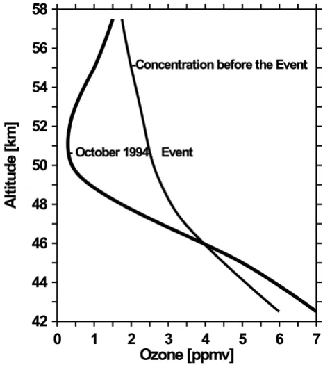
For the ozone decrease event of October 1994 Fig. 2 illus-trates this behavior depicting smoothed nighttime height pro-files of the local ozone hole compared with the corresponding mean values of a period of 1 month before the hole occurred as a reference profile. The individual values of measurement drop partly below 0.5 ppmv within the local ozone hole. At about 55 km the ozone concentration begins to decrease and reaches its strongest decline at about 50 to 52.5 km. At about 45 km the effect begins to reverse and even shows an increase finally at 42.5 km. Surprisingly, the nighttime values drop somewhat below the corresponding daytime values during the decreasing phase, whereas no significant diurnal variation has been found outside this. We also note that the absolute ozone values (in cm−3)display a local minimum there.
As the characteristic chemical time of the odd oxygen-odd hydrogen system (consisting of the main chemical active species O3, O, O(1D)-H, OH, HO2)amounts to about one
day around the stratopause, the ozone decrease events can-not be explained by direct transport of air poor in ozone (the chief odd oxygen constituent there) from remote areas. How-ever, parameters such as the temperature and the water vapor concentration can change their magnitude considerably with a time scale in the order of some days to few weeks. The average thermal behavior of the extended stratopause region in mean latitudes according to CIRA-86 is given by warm air in summer (274 K, 50◦, 50 km, June) and cold air in winter (253 K, 50◦, 50 km, December). The average temperature for September/October ranges around 260 K. This general feature is interrupted in the winter season by the so-called sudden stratospheric warmings when the polar vortex breaks down and the air can be heated up to more than 300 K.
Fig. 2. The figure displays a vertical section through the local ozone hole of the October 1994 event compared with a smoothed profile of a 1 month mean before the episode began. Below about 46 km the effect reverses due to small water vapor mixing ratios there during the event.
The water vapor concentration possesses a marked an-nual variation in mean and high latitudes characterized by a concentration peak up to more than 7 ppmv just around the stratopause/lower mesosphere occurring from August to Oc-tober (e.g. Seele and Hartogh, 1999; K¨orner and Sonnemann, 2001; Sonnemann and Grygalashvyly, 2005). Model calcula-tions predict only a relatively slight dependence of the ozone concentration on temperature (according to the dependence of the reaction rates on temperature), water vapor or even on chlorine when it varies in natural borders (Frederick, 1980; Rusch et al., 1983; Solomon et al., 1983; Keating et al., 1985; Fichtelmann and Sonnemann, 1989).
2 Water vapor observations and temperature measurements
Oct 1 Jan 1 Apr 1 Jul 1 Oct 1 time (month) 40 50 60 70 80 Hö he ( km ) 0.0 1.0 2.0 3.0 4.0 5.0 6.0 7.0 8.0 9.0 10.0 vo lume m ix in g r a tio ( ppm )
Oct 1 Jan 1 Apr 1 Jul 1 Oct 1
time (month) 40 50 60 70 80 Hö he ( km ) 0.0 1.0 2.0 3.0 4.0 5.0 6.0 7.0 8.0 9.0 10.0 vo lume m ix in g r a tio ( ppm ) 1.0 2.0 2.0 3.0 3.0 3.0 4.0 4.0 4.0 5.0 5.0 5.0 6.0 6.0 6.0 6 .0 6.0 6.0 6 .0 6.0
7.0 7.0
7.0 7.0 7.0 7.0 7 .0 7.0 7.0 7 .0 8 .0 8.0 8 .0 8.0 1994 1995
Fig. 3. Water vapor measurements at the same place of ozone
ob-servation showing very strong events of enhancements of the H2O
mixing ratio simultaneously to the ozone decrease events.
from anywhere afar to the region of observation (see also dis-cussion in Seele and Hartogh, 2000). The role of water vapor for the chemistry in the mesosphere/stratopause region was discussed in detail by Sonnemann et al. (2005). Water vapor is the main source gas for the chemically rather active hy-drogen radicals which destroy catalytically odd oxygen. The effective chemical lifetime of water vapor at the stratopause, that is the lifetime which considers both the chemical loss and the chemical production (see K¨orner and Sonnemann, 2001 for definition), is extremely long and amounts to several months meaning water vapor is determined by transports in this domain. The hydrogen radicals formed by the photolysis of water vapor and their oxidation by O(1D) return to water vapor within so-called zero cycles (Sonnemann et al., 2005) producing only heat. Hence the place where these strange humid air bubbles came from and the source of the humid-ity are open questions. The feature looks like air welling up, but this statement is speculative. A possible cause taken into consideration is the exhaust of rockets. There were three launches of major rockets from Cape Canaveral in the weeks preceding each of the observed local ozone decrease events in mid-to-late October of 1994, in mid-January of 1995 and a third hint in early June 1995. These dates correspond to the launches of SST-68 on 30 September 1994 and Titan IV rocket on 22 December 1994 and 14 May, 1995. However, the measured water vapor bubbles last longer than a week and the vertical extension is in the order of 10 km or more begin-ning at 45 km for the October event. Even for a slow zonal wind speed of the middle atmospheric wind jet during this event the zonal extension of the bubble would amount thou-sands of kilometers. This is definitely too large for a rocket cloud of exhaust. It was found by means of balloon measure-ments a strong increase of the stratospheric water vapor in the past before 2000 (Oldmans and Hofmann, 1995; Evans et al., 1998) which could only be explained to 40% by the
Lindau: Lat. 51.65 Long. 10.1
200 200 200 200 200 210 210 210 210
210 210 210
210 210 210 220 220 220 220 220 220 220 220 220 220 220 230 230 230 230 230 240 240 240 240 240 240 250 250 250 250 250 250 250
250 250 250
260 260 260 260 260 260 260 260 260 260 260 260 270 270 270 270 280 280
Oct 01 ’94 Jan 01 ’95 Apr 01 ’95 Jul 01 ’95 Oct 01 ’95 Jan 01 ’96
Time 20 30 40 50 60 Altitude [km] 20 30 40 50 60 200 220 240 260 280 Temperature [K]
/t /h / / df li/ ll tiO t242002 1/t t fil /199407 199512/ l t /t 199407 199512 2d W d J 12 16 21 12 2005
Fig. 4. Temperature measurements up to 52 km by the National Center for Environmental Prediction for a latitude corresponding to that of Lindau. Above that height the temperature has been gradually adopted to the MSIS-model. The measurements indicate a stratospheric warming during the January 1995 ozone decrease event and a moderate enhancement for the October 1994 episode.
methane increase (Foster and Shine, 1999) and thus it seems to be unexplained (Kley et al., 2000). Possibly, an enhanced water vapor content of the stratosphere results from singular events of water vapor injection from the troposphere.
Figure 4 exhibits the smoothed temperature between 20 and 60 km including the period considered according to mea-surements of the National Center for Environmental Predic-tion (McPherson et al., 2000) up to 52 km. Above this height the measurements have been gradually adapted to the MSIS model data (Hedin, 1991). Evidently the ozone decrease events and water vapor enhancements are connected with a (slight) increase of the temperature, additionally chemi-cally influencing the ozone decrease and possibly entailing a welling up of humid air, perhaps connected with a meridional transport of more humid air from the north. The temperature increase, according to these smoothed data, is not so marked during the October event but it seems to be connected with a stratospheric warming for the event in January 1995.
3 Ozone dissociation frequency
Ozone is the only chemically variable constituent of which dissociation frequency depends on its column density. (The ozone dissociation rate is the product of the ozone dissoci-ation frequency with the concentrdissoci-ation of ozone.) The dis-sociation frequency of molecular oxygen also depends on the O2-column density, but its dissociation frequency is too
small to influence the O2-density noticeably. For all other
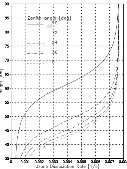
Fig. 5. Ozone dissociation frequency for 5 different solar zenith angles. The strongest decrease of the frequency with decreasing
height for solar zenith angles greater than 54◦takes place around
the stratopause.
dissociation frequencies. E.g. the dissociation frequency of water vapor at a certain height is chiefly determined by the absorption by O2. The absorption by water vapor itself plays
no role. The dissociation of ozone results in the formation of atomic oxygen, mainly in the exited state O(1D). O(1D) is chemically a rather active species oxidizing H2O, H2and
CH4forming hydrogen radicals which destroy ozone
catalyt-ically. However, the greatest part of O(1D) atoms is subjected to quenching reactions by collisions with air molecules re-sulting in atomic oxygen in the ground state, and the largest part of atomic oxygen returns to ozone again by the important three-body reaction O+O2+M→O3+M depending
quadrati-cally on the air density. But an increase of the flowing equi-librium of O and an amplified formation of hydrogen radicals destroy odd oxygen and influences the catalytic cycles in that they become more effective. On the one hand atomic oxygen reacts with ozone. On the other hand an effective catalytic cycle consists of the following three reactions:
O+OH→O2+H
H+O2+M→HO2+M
HO2+O→OH+O2
net: O+O→O2
Figure 5 displays the ozone dissociation frequency for 5 different solar zenith angles χ including 54◦, which is approximately the solar zenith angle at noon at Lindau during equinox. The dissociation frequencies are taken from Fichtelmann and Sonnemann (1989), Sonnemann et al. (1998) and R¨oth (1992). They combine a code developed for thermospheric-mesospheric as well as for stratospheric models and are used in the GCMs COMMA-IAP (COlogne Model of the Middle Atmosphere of the Institute of Atmo-spheric Physics, e.g. Sonnemann et al., 2005) and LIMA (Leibniz-Institute Middle Atmosphere model, e.g. Sonne-mann et al., 2008). The dissociation frequency is almost constant within the whole mesosphere, with the exception of the lowermost domain. The absorption cross section of ozone has an order of 10−17cm2, meaning the column den-sity of ozone needs an order of 1017cm−2to produce an
opti-cal depth of unity. The column density at a certain altitude is given by the product of the density at this height with a mean density scale height along the penetration path of absorbed radiation multiplied by the Chapman-function Chχ (≈secχ
for χ≤75–80◦). The Chapman-function takes the increase of the column density along the penetration path of the in-cident radiation of a zenith angle χ into calculation. The density scale height along the penetration path of radiation is not constant; it depends on height and, less strongly, on
χ. The mean scale height is that equivalent value (depending on height and zenith angle) that the column densities calcu-lated on the one hand with the mean scale height and on the other hand with the real variable density scale height is the same. A coarse value for the ozone density scale height is 5 km. Hence, a noticeable decrease of the ozone dissociation frequency starts not much before the ozone density reaches an order of 1010cm−3(meaning the optical depthτ for
242.4 nm in the Herzberg continuum with an extreme small cross section. The main photolysis of molecular oxygen in the domain under consideration takes place in the Schumann-Runge bands with wavelength below 200 nm. The main dis-sociation of ozone takes place in the Hartley bands around 250 nm and thus, the stronger radiation does not worth men-tioning dissociate O2 but penetrates only somewhat deeper
into the atmosphere. A further negative feedback which has to take into consideration results from the fact that on the one hand the dissociation frequency increases, but on the other hand with decreasing ozone concentration the dissociation rate (being the product of increasing dissociation frequency and decreasing ozone concentration which determines the production term of atomic oxygen) is damped.
4 A simplified chemical model of the ozone dissociation rate-ozone column density feedback
Usually, the description of details of the current global mod-els in the publications is very limited and therefore, it is diffi-cult to judge whether or not this feedback has been correctly considered. Normally, the models use ozone dissociation frequencies given as tables calculated for discrete steps of height or of pressure and of the solar zenith angle (possibly still depending on season and latitude). In order to investi-gate the behavior of the chemical system when considering this feedback, we developed a simple dynamical model. The height in the model under consideration was determined by the aeronomical conditions, such as the density of air and consequently of molecular oxygen, molecular hydrogen of 0.5 ppmv and other constituents and the dissociation frequen-cies of water vapor and molecular oxygen etc. The water va-por mixing ratio, the temperature, the ClOx-mixing ratio then
act as control parameters. (A control parameter is a param-eter fixed for each model run which is stepwise increased or decreased from one model run to the next one using the old final values as new initial values.)
All chemically active constituents, i.e. constituents of the odd oxygen (O, O3, and O(1D)), the odd hydrogen (H, OH,
HO2, and H2O2)and the odd nitrogen families (N(4S), NO,
NO2, NO3), are integrated separately meaning not as family.
We integrate the stiff chemical system with a self-adjusting time step in the way that the largest absolute change of the concentration of any constituent does not exceed 1 per mil. This procedure was employed to calculate the bifurcation diagram of the non-linear response of the chemical system in the mesopause region which requires highest precision to determine the bifurcation points (e.g. Fichtelmann and Son-nemann, 1992; Sonnemann and Fichtelmann, 1997; Sonne-mann and Feigin, 1999). The method of self-adjusting time step was also used by McKenna et al. (2002) to calculate the ozone chemistry within the polar vortex. The chemical code including the chemical reaction rates are taken from our 3-D models (e.g. Sonnemann et al., 1998, 2005, 2008;
Hartogh et al., 2004). The ClOx-mixing ratio was taken
as constant for each model run but the partitioning between the share of Cl and ClO was variable depending on the odd oxygen chemistry. The mesosphere and the stratopause re-gion (above about 40 km) can widely be described by a pure odd oxygen-odd hydrogen chemistry (Crutzen et al., 1995), but below that domain the catalytic ozone destruction by the chlorine species becomes increasingly important so that we also consider the ozone decomposition by these constituents. NOx-species were considered but they play no role in that
domain. In this context we also have checked that no solar proton event occurred during the time of the ozone decrease events observed. The sensitivity was studied with regard to the O2-dissociation frequency and the air density
(pres-sure change). The most important question is how does the ozone dissociation frequency depend on the locally calcu-lated ozone concentration? The answer requires assumptions about the ozone distribution above the height under consid-eration.
The ozone column density determines the ozone dissoci-ation frequency. The ozone column density used for calcu-lation of the dissociation frequency is given, as mentioned above, by
NO3(z, t, χ )=nO3(z, t )HO3(z, t )Ch(χ ) (1)
depending on heightz, timetand the solar zenith angleχ (t ).
nO3(z, t )is the ozone density atz,HO3(z, t )stands for the
mean density scale height of ozone at zalong the path of penetration of radiation (it depends only little onχ ). For the mean scale height we used the expression
xH
O3(z,t)=0HO3(z,0)(nO3(z,0)/nO3(z, t ))
(1−x) (2)
The argument t indicates the time depending ozone val-ues calculated by the model and 0 stands for a constant model value determining the dissociation frequency in the conventional case without consideration of the feedback (nO3(50,0)=2.4 ppmv). A value x=1 means that the mean
density scale height of ozone 1HO3(z, t )=
0H
O3(z,0) does
not depend on the time-dependingnO3(z,t) in the model (a
strong feedback case). In this case, the ozone dissociation frequency at a constant altitude depends directly on the local ozone density, meaning the mean scale height stays constant at a value given before the calculation. Values between 1 and 0 increasingly soften the positive feedback and values greater than unity would strengthen it. Values less than zero are pos-sible if an ozone bulge occurs.
5 Model calculations by means of a simplified model
Fig. 6a. Nighttime ozone mixing ratios at 50 km for equinox con-ditions and a water vapor mixing ratio of 8 ppmv depending on the
feedback parameterx. The parameter is the temperature. The
sys-tem creates a trigger solution only for high feedback parameters and lower temperatures, but generally the ozone values decreases with increasing feedback parameters having values as low as be-low 0.5 ppmv already for moderate feedback parameters and higher temperatures.
special aeronomical conditions. The calculations help to un-derstand the phenomenon observed. A real calculation of this phenomenon is only possible in the frame of a completely in-teractively operating 3-D-model which computes the ozone dissociation frequency of each time step on the basis of the current ozone distribution within the whole height range; but according to our knowledge such a model is not yet available. We show results here according to the latitude of Lindau at 50 and 45 km altitude for equinox (half a day sunshine).
The feedback is restrained to a certain extent by an in-crease of the mean scale height determining the ozone col-umn density without, of course, compensating for the effect completely. The only relevant magnitude determining the ozone dissociation frequency is the ozone column density. Fig. 6a displays calculations of an example for a water va-por mixing ratio of 8 ppmv according to the observation in the period of strongest ozone decrease. Although the dif-ferences between daytime and nighttime values are small, we show generally nighttime values. The control parame-ter is, according to Eq. (2), the exponent 1-xconsidering the power of feedback. The parameter for the individual curves is the temperature. A trigger solution exists for smaller tem-peratures but only under the assumption of strong feedback (small values of 1-x). Apart from that, the curves decrease monotonically with increasing feedback, however, the gradi-ent becomes steeper with dropping off temperatures within a certain interval of the control parameter. It is an important result that, particularly for higher temperatures, the ozone mixing ratios fall below 0.5 ppmv even for weaker feedbacks and that the upper solution cannot be taken on for x-values less than unity. The simple reason for this latter assertion
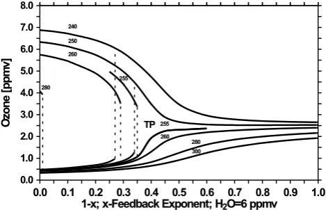
re-Fig. 6b. The same state of affairs as depicted in re-Fig. 6a but for
6 ppmv H2O mixing ratio. The diagram is more complicated now.
The feedback results in increasing ozone mixing ratios for lower temperatures (the critical temperature is about 254.1 K) whereas for higher temperature the values decrease. A trigger solution exists for x-values greater than 0.61.
sults from the fact that, under natural conditions, the system starts from a catchment region which belongs to the lower solution.
Figure 6b shows the same state of affairs as displayed in Fig. 6a but for a water vapor mixing ratio of 6 ppmv. This value corresponds more to mean conditions. Also in this case the upper trigger solution occurs only for a stronger feed-back. There is a triple point for 254.1 K at about 1-x=0.39 and a ozone mixing ratio of 2.48 ppmv. For temperatures greater than this value, the ozone concentration decreases monotonically with decreasing feedback parameter 1-x but a trigger solution exists for values less than a certain criti-cal value (1-x)c which depends on temperature. The larger
the temperature the smaller (1-x)cis. For temperatures less
than 254.1 K the ozone concentration increases monotoni-cally with decreasing feedback parameters and a trigger so-lution also occurs for feedback parameter values less than the temperature depending on values (1-x)c. Obviously, a strong
ozone enhancement at 50 km has not been observed thus far. It would require that the ozone column density is very high, meaning the ozone density has to be high over a sufficiently extended height interval above the altitude considered. This possibility is, however, reduced by the fact that with increas-ing height the ozone amplification effect becomes more in-efficient so that the feedback parameter does not have suffi-ciently large values.
Figure 6c depicts calculations according to a height of 45 km. The control parameter is the water vapor mixing ra-tio and the parameter of the individual curves is the feedback parameter 1-x. The temperature amounts to 260 K,nO3(0)
corresponds to 4.5 ppmv now, it is ClOx=0.4 ppbv.
forT=260 K. There is a trigger solution for large feedback parameter values only. The critical H2O mixing ratio for a
state transition is shifted to greater values for smaller temper-atures. Considering the episode from October 1994 the sys-tem stayed in the upper solution due to the relatively low H2O
mixing ratios and moderate temperature at 45 km. This is, at least, the common case at that height. Instead, the ozone-ozone dissociation rate feedback may normally increase the ozone mixing ratio at this and lower altitudes compared with results not considering the feedback.
6 Discussion
Multiple publications have dealt with the so-called ozone deficit problem consisting in a systematic underestimation of ozone by the standard models (e.g. Clancy et al., 1987; Eluszkiewicz and Allen, 1993; Siskind et al., 1995; Summers et al., 1996, 1997; Dessler et al., 1998). A more detailed de-scription of the employed models is usually not given. Thus, perhaps there is a systematic underestimation of the ozone-ozone dissociation rate feedback by the models in the domain of the upper stratosphere. However, in contrast to this asser-tion (Crutzen et al., 1995) did not find evidence for an ozone deficit.
We have estimated the feedback parameterx depending on height for the October 1994 episode according to the smoothed values shown in Fig. 2. The parameterxhas been calculated on the basis of expression (2). The mean density scale height is generally defined by
H (z)=
Z ∞
z
exp −z 0
−z
H (z0)
!
dz0. (3)
The density scale heightH(z0)can be derived approximately from the measured density values. Both the curves of Fig. 2 yield a different mean scale height.xHresults from the curve of the observed local ozone hole values and 0H from the curve representing the densities before the event arose. Com-ing from high altitudes, the parameter 1-x used in Fig. 6a, b as a control parameter slowly begins to increase. At 50 km the value amounts to about 0.64 and at 49 km to about 0.38. The zero line is crossed between 48 and 49 km. A pole occurs between 45 and 46 km wherexbecomes infinity and changes its sign for lower heights. For further decreasing heights the negative values seems to approach zero again. The pole is de-termined when the hole becomes a bulge below 45 to 46 km. Approximately at this height the mean density scale height has its smallest value with 2.7 km whereas the value for the reference case is about 4.7 km. We have to keep in mind that the measured ozone values are averaged over 7–10 km and smoothed after that and the reference values are only an approximated estimate. In particular, those ozone mixing ratios observed around the minimum cannot be determined accurately. The temperature is not precisely known and is
Fig. 6c. Nighttime ozone mixing ratios for equinox conditions and
T=260 K at 45 km depending on the water vapor mixing ratio. The
parameter is the feedback parameter. Additionally the figure shows
the curve forT=250 K andx=1. The system produces the lower
ozone solution only for very strong feedback parameters values and
high H2O mixing ratios.
probably underestimated. Despite these restrictions, the x-value around 49 km corresponding to the lower state agrees surprisingly well with the results shown in Fig. 6a for 50 km. Evidently, at 45 km and below there is only one solution for a water vapor concentration of 8 ppmv and negative x-values corresponding to the upper state. Normally the water vapor mixing ratio is not so large and consequently the system re-sponse is not so strong. Depending on the temperature, the ozone values can slightly decrease or increase compared with the case ofx=0 as Fig. 6b illustrates.
In context with the decline of the ozone layer due to the anthropogenic impact by ClOx and NOx the first sign of a
a natural variability such as the Brewer-Dobson circulation connected with exchange processes between troposphere and stratosphere (Foster and Shine, 1999). The global circulation also influences the water vapor transport in the mesosphere of high latitudes. On the other hand, a cooling of the middle at-mosphere by the increasing CO2-concentration should soften
this effect. Possibly, the negative feedback by the reduced ozone concentration as the main absorber of UV-radiation being the chief energy input into the middle atmosphere is more important. This effect cannot, of course, compensate for the ozone reduction but it can only reduce the decline to a certain extent.
7 Trigger solutions in chemical systems of the atmo-sphere and conclusions
The possibility of trigger solutions of the chemical systems within the atmosphere was first introduced by Prather et al. (1979) and Fox et al. (1982) for a simplified system of the stratospheric odd nitrogen chemistry. Later on vari-ous researchers (White and Dietz, 1984; Kasting and Ack-ermann, 1985; Kleinman, 1991; Zimmermann and Poppe, 1993; Stewart, 1993; Poppe and Lustfeld, 1996; and other groups) discussed a low and high ozone regime in the chem-istry of the boundary layer. Under consideration of vertical transport Yang and Brasseur (1994) found a trigger solution in the chemistry of the mesosphere and finally Feigin and Konovalov (1996) discovered a multiple solution in the high-latitude stratospheric photochemical system.
The investigations by means of an idealized model do not fit the reality in any case. Hence, it is not clear whether the natural system operates in a bistable mode under particular conditions or not. In the positive case we expect that only the lower ozone solution can occur in the range of positive x-values, whereas in the lower domain for negative x-values the upper solution may prevail. The transition regions from the lower to an upper solution have not been considered. The oc-currence of a lower solution requires very high water vapor mixing ratios and high temperatures (such as occur during stratospheric warmings) within a sufficiently extended height range around the stratopause. Definitely, as Fig. 6a demon-strated, the ozone mixing ratio drops below 1 ppmv for rel-atively weak feedback parameters and even below 0.5 ppmv for stronger ones. Such strong events have been observed.
The search for similar events in the data of the latest years until 2008 revealed different episodes of ozone de-crease, but, in contrast to the expected behavior, they were not so marked as those in the early nineteenth. During the episodes after 1999 the ozone mixing ratios declined from more than 2 ppmv to minimum 1 ppmv, sometimes con-nected with stratospheric warmings, but decrease events also occurred in summer. There are also events of sudden ozone enhancements in winter characterized by values larger than 3.5 ppmv. Unfortunately, there were no simultaneous
wa-ter vapor measurements at Lindau. However, measurements in ALOMAR showed a general decrease of the water va-por concentration since 2000 after a phase of considerable increase. As reported by Randel et al. (2006) and Scherer et al. (2008) the Brewer-Dobson circulation in the tropics changed abruptly after 2001 impacting the water vapor dis-tribution in the lower stratosphere. Bittner et al. (2000) and H¨oppner and Bittner (2007) found a slowdown of the planetary wave activity also in middle latitudes. Particu-larly the values during the winter season became noticeable smaller what could explain that the latest events were less pronounced. Thus the enhancement episodes could be linked with episodes of strong water vapor decrease. Pronounced ozone decrease episodes are very few events occurring under exceptionally favorable conditions of very large water vapor concentrations in the order of 8 ppmv and additionally high atmospheric temperatures. In this case real state transitions seems to be possible whereas normally only an amplified ozone change takes place indicated by the high short-term variability of ozone around the stratopause resulting from the ozone-ozone dissociation rate feedback.
It is very interesting to note that in the Martian atmo-sphere the ozone dissociation frequency also depends on the ozone concentration itself. The main Martian constituent CO2 has only a very small absorption cross section in the
Hartley bands. A discrepancy between ozone measurements and model calculations (Lef`evre et al., 2004) between 30 and 60 km altitude was stated in Lebonnois et al. (2006). This is just the height range in which the ozone dissociation fre-quency strongly decreases with decreasing height.
Acknowledgements. This work was supported by the German
Re-search Community DFG, grant So 268/4-1.
We greatly appreciate the assistance of Christopher Jarchow and Michailo Grygalashvyly in preparing some plots.
The service charges for this open access publication have been covered by the Max Planck Society.
Edited by: U. Feudel
Reviewed by: two anonymous referees
References
Bittner, M., Offermann, D., and Graef, D.: Mesopause tempera-ture variability above midlatitudev station in Europe, J. Geophys. Res., 105, 2045–2058, 2000.
CIRA-86: Part II Middle Atmosphere Models, edited by: Rees, D., Barnett, J. J., Labitzke, K. Clancy, R. T., and Rusch, D. W., So-lar Mesosphere Explorer Temperature Climatology of the meso-sphere as compared to CIRA Model, Adv. Space Res., 10(12), 187–206, 1986.
Crutzen, P. J., Grooß, J.-U., Br¨uhl, C., M¨uller, R., and Russel III, J. M.: A reevaluation of the ozone budget with HALOE UARS data: No evidence of the ozone deficit, Science, 268, 705–708, 1995.
Dessler, A. E., Burrage, M. D., Grooss, J.-U., et al.: Selected sci-ence highlights from the first 5 years of the Upper Atmospheric Research Satellite (UARS) program, Rev. Geophys., 36, 183– 210, 1998.
Dlugokencky, E. J., Houweling, S., Bruhwiler, L., Masarie, K. A., Lang, P. M., Miller, J. B., and Tans, P. P.: Atmospheric methane levels off: Temporary pause or a new steady-state?, Geophys. Res. Lett., 30, 1992, doi:10.1029/2003GL018126, 2003. Eluszkiewicz, J. and Allen, M.: A global analysis of the ozone
deficit in the upper stratosphere and lower mesosphere, J. Geo-phys. Res., 98, 1069–1082, 1993.
Evans, S. J., Toumi, R., Harries, J. E., Chipperfield, M. P., and Rus-sel, J. M.: Trends in stratospheric humidity and the sensitivity of ozone to these trends, J. Geophys. Res., 103, 8715–8725, 1998. Feigin, A. M. and Konovalov, I. B.: On the possibility of the
com-plicated dynamic behavior of atmospheric photochemical sys-tem: Instability of the Antarctic photochemistry during ozone hole formation, J. Geophys. Res., 101, 26023–26038, 1996. Fichtelmann, B. and Sonnemann, G.: On the variation of ozone
in the upper mesosphere and lower thermosphere: A compari-son between theory and observation, Z. Meteorol., 39, 297–308, 1989.
Fichtelmann, B. and Sonnemann, G.: Non-linear behaviour of the photochemistry of minor constituents in the mesosphere, Ann. Geophys., 10, 719–728, 1992.
Foster, P. M. de F. and Shine, K. P.: Stratospheric water vapour changes as a possible contributor to observed stratospheric cool-ing, Geophys. Res. Lett., 26, 3309–3312, 1999.
Fox, J. L., Wofsy, S. C., McElroy, M. B., and Prather, M. J.: A stratospheric chemical instability, J. Geophys. Res., 87, 11126– 11132, 1982.
Frederick, J. E.: Seasonal variations in high-latitude ozone and metastable molecular oxygen emissions: A theoretical interpre-tation, J. Geophys. Res., 85, 1611–1617, 1980.
Hedin, A.: Extension of the MSIS thermosphere model into the middle and lower atmosphere, J. Geophys. Res., 96, 1159–1167, 1991.
Kasting, J. F. and Ackerman, T. P.: High atmospheric NOxlevels
and multiple photochemical steady states, J. Atmos. Chem., 3, 321–340, 1985.
Hartogh, P., Jarchow, C., Sonnemann, G. R., and Grygalashvyly, M.: On the spatiotemporal behavior of ozone within the meso-sphere/mesopause region under nearly polar night conditions, J. Geophys. Res., 109, D18303, doi:10.1029/2004JD004576, 2004. Keating, G. M., Brasseur, G. P., Nicholson III, J. Y., and de Rudder, A.: Detection of the response of ozone in the middle atmosphere to short-term solar ultraviolet variations, Geophys. Res. Lett., 12, 449–452, 1985.
Khalil, M. A. K., Rasmussen, R. A., and Moraes, F.: Atmospheric methane at Cap Meares: Analysis of a high-resolution data base and its environmental implications, J. Geophys. Res., 98, 14753– 14770, 1993.
Kheshgi, H. S., Jain, A. K., Kotamarthi, V. R., and Wuebbles, D. J.: Future atmospheric methane concentrations in the context of stabilization of greenhouse gas concentrations, J. Geophys. Res.,
104, 19183–19190, 1999.
Kleinman, L. I.: The low and high NOxregime, J. Geophys. Res.,
96, 20721–20733, 1991.
Kley, D. J., Russell III, M., and Phillips, C. (Eds.): SPARC As-sessment of Upper Tropospheric and Stratospheric Water Vapor, SPARC Tech. Rep., 2, 312 pp., 2000.
K¨orner, U. and Sonnemann, G. R.: Global 3D-modeling of wa-ter vapor concentration of the mesosphere/mesopause region and implications with respect to the NLC region, J. Geophys. Res., 106, 9639–9651, 2001.
Lebonnois, S., Qu´emerais, E., Montmessin, F., Lef`evre, F.,
Per-rier, S., Bertaux, J.-L., and Forget, F.: Vertical
distribu-tion of ozone on Mars as measured by SPICAM/Mars Ex-press using stellar occultations, J. Geophys. Res., 111, E09S05, doi:10.1029/2005JE002643, 2006.
Lef`evre, F., Lebonnois, S., Montmessin, F., and Forget, F.: Three-dimensional modeling of ozone on Mars, J. Geophys. Res., 109, E07004, doi:10.1029/2004JE002268, 2004.
McKenna, D. S., Groß, J.-U., G¨unther, G., Konopka, P., M¨uller, R., Carver, G., and Sasano, Y.: A new chemical Lagrangian model of the stratosphere (CLaMS) 2. Formulation of chemistry scheme and initialization, J. Geophys. Res., 107(D15), 4256, doi:10.1029/2000JD000113, 2002.
Mcpeters, R. D.: The Behavior of Ozone Near the Stratopause From Two Years of BUV Observations, J. Geophys. Res., 85(C8), 4545–4550, 1980.
McPherson, R. S., Bergman, K. H., Kistler, R. E., Rasch, G. E., and Gordon, D. S.: The NMC Operational Global Data Assimilation System, Mon. Weather Rev., 107, 1445–1461, 1979.
Oldmans, S. J. and Hofmann, D. J.: Increase in lower stratospheric water vapour and a midlatitude northern hemisphere site from 1981–1994, Nature, 374, 146–149, 1995.
Poppe, D. and Lustfeld, H.: Nonlinearities in the gas phase chem-istry of the troposphere: Oscillating concentrations in a simpli-fied mechanism, J. Geophys. Res., 101, 14373–14380, 1996. Prather, M. J., McElroy, M. B., Wofsy, S. C., and Logan, J. A.:
Stratospheric chemistry: Multiple solutions, Geophys. Res. Lett., 6, 163–164, 1979.
Randel, W. J., Wu, F., V¨omel, H., Nedoluha, G. E., and
Forster, P.: Decreases in stratospheric water vapor after
2001: Links to changes in the tropical tropopause and the Brewer-Dobson circulation, J. Geophys. Res., 111, D12312, doi:10.1029/2005JD006744, 2006.
Rasmussen, R. A. and Khalil, M. A. K.: Atmospheric methane in the recent and ancient atmospheres: Concentrations, trends, and interhemispheric gradients, J. Geophys. Res., 89, 11599–11605, 1984.
Reinsel, G. C., Tiao, G. C., DeLuisi, J. J., Mateer, C. L., Miller, A. J., and Frederick, J. E.: Analysis of upper stratospheric Umkehr ozone profile data for trends and the effects of stratospheric aerosols, J. Geophys. Res., 89, 4833–4840, 1984.
Reinsel, G. C., Tiao, G. C., Miller, A. J., Wuebbles, D. J., Connell, P. S., Mateer, C. L., and DeLuisi, J. J.: Statistical analysis of total ozone and stratospheric Umkehr data for trends and solar cycle relationship, J. Geophys. Res., 92, 2201–2209, 1987.
R¨oth, E.-P.: Fast algorithm to calculate the photon flux in opti-cally dense media for use in photochemical models, Ber. Bunsen-Gesellsch, Phys. Chem., 96, 417–420, 1994.
R. J., Thomas, G. E., Sanders, R. W., Lawrence, G. N., and Eck-man, R. S.: Ozone density in the lower mesosphere measured by a limb scanning ultraviolet spectrometer, Geophys. Res. Lett., 10, 241–244, 1983.
Scherer, M., V¨omel, H., Fueglistaler, S., Oltmans, S. J., and Staehe-lin, J.: Trends and variability of midlatitude stratospheric water vapour deduced from the re-evaluated Boulder balloon series and HALOE, Atmos. Chem. Phys., 8, 1391–1402, 2008,
http://www.atmos-chem-phys.net/8/1391/2008/.
Seele, C. P. and Hartogh, P.: Water vapor of the polar middle at-mosphere: Annual variation and summer mesosphere conditions as observed by ground-based microwave spectroscopy, Geophys. Res. Lett., 26, 1517–1720, 1999.
Seele, C. P. and Hartogh, P.: A case study on middle atmospheric water vapor transport during the February 1998 stratospheric warming, Geophys. Res. Lett., 27, 3309–3312, 2000.
Siskind, D. E., Connor, B. J., Eckman, R. S., Remsberg, E. E., Tsou, J. J., and Parrish, A.: An intercomparison of model ozone deficits in the upper stratosphere and mesosphere from two data sets, J. Geophys. Res., 100, 11191–11201, 1995.
Solomon, S., Rusch, D. W., Thomas, R. J., and Eckman, R. S.: Comparison of mesospheric ozone abundances measured by the Solar Mesospheric Explorer and model calculations, Geophys. Res. Lett., 10, 249–252, 1983.
Sonnemann, G.: On the formation of particlelike pattern, the ampli-tude modulated route to chaos and the wave-particle dualism in three-dimensional systems under global constraints, Prog. Theor. Phys., 99(6), 931–962, 1998.
Sonnemann, G. and Fichtelmann, B.: Subharmonics, cascades of period doubling, and chaotic behavior of photochemistry of the mesopause region, J. Geophys. Res., 102, 1193–1203, 1997. Sonnemann, G., Kremp, Ch., Ebel, A., and Berger, U.: A
three-dimensional dynamic model of minor constituents of the meso-sphere, Atmos. Environm., 32, 3157–3172, 1998.
Sonnemann, G. R. and Feigin, A. M.: Nonlinear behavior of a reaction-diffusion system of the photochemistry within the mesopause region, Phys. Rev. E, 59, 1719–1726, 1999. Sonnemann, G. R. and Grygalashvyly, M.: Solar influence on
meso-spheric water vapor with impact on NLCs, J. Atmos. Sol.-Terr. Phy., 67, 177–190, 2005.
Sonnemann, G. R., Grygalashvyly, M., and Berger, U.: Autocat-alytic water vapor production as a source of large mixing ratios within the middle to upper mesosphere, J. Geophys. Res., 110, D15303, doi:10.1029/2004JD005593, 2005.
Sonnemann, G. R., Hartogh, P., Jarchow, C., Grygalashvyly, M., and Berger, U.: On the winter anomaly of the night-to-day ratio of ozone in the middle to upper mesosphere in middle to high latitudes, Adv. Space Res., 40, 846–854, 2007.
Sonnemann, G. R., Hartogh, P., Grygalashvyly, M., Li, S., and Berger, U.: The quasi 5-day signal in the mesospheric water va-por concentration in high latitudes in 2003 – a comparison be-tween observations at ALOMAR and calculations, J. Geophys. Res., 113, D04101, doi:10.1029/2007JD008875, 2008.
Stewart, R. W.: Multiple steady states in atmospheric chemistry, J. Geophys. Res., 98, 20601–20611, 1993.
Stewart, R. W.: Dynamics of the low to high NOxtransition in a
simplified tropospheric photochemical model, J. Geophys. Res., 100, 8929–8943, 1995.
Summers, M. E., Conway, R. R., Siskind, D. E., Bevilacqua, R.,
Strobel, D. F., and Zasadil, S.: Mesospheric HOx
photochem-istry: Constraints from recent satellite measurements of OH and
H2O, Geophys. Res. Lett., 23, 2097–2100, 1996.
Summers, M. E., Conway, R. R., Siskind, D. E., Stevens, M. H., Offermann, D., Riese, M., Preusse, P., Strobel, D. F., and Russel III, J. M.: Implications of satellite OH observations for middle
atmospheric H2O and ozone, Science, 277, 1967–1970, 1997.
Thomas, G. E., Olivero, J. J., Jensen, E. J., Schr¨oder, W., and Toon, O. B.: Relation between increasing methane and the presence of ice clouds at the mesopause, Nature, 338, 490–492, 1989. Thomas, G. E. and Olivero, J. J.: Noctilucent clouds as possible
indicators of global change in the mesosphere, Adv. Space Res., 28(7), 937–946, 2001.
White, W. H. and Dietz, D.: Does the photochemistry of the tropo-sphere admit more than one steady state?, Nature, 309, 242–244, 1984.
Yang, P. and Brasseur, G.: Dynamics of the oxygen-hydrogen sys-tem in the mesosphere, 1. Photochemical equilibria and catastro-phe, J. Geophys. Res., 99, 20955–20965, 1994.
Zimmermann, J. and Poppe, D.: Nonlinear chemical couplings
in the tropospheric NOx-HOx gas phase chemistry, J. Atmos.