www.clim-past.net/7/1149/2011/ doi:10.5194/cp-7-1149-2011
© Author(s) 2011. CC Attribution 3.0 License.
Climate
of the Past
Corrigendum to
“Upper ocean climate of the Eastern Mediterranean Sea during the
Holocene Insolation Maximum – a model study” published in Clim.
Past, 7, 1103–1122, 2011
F. Adloff1,2, U. Mikolajewicz1, M. Kuˇcera3, R. Grimm1,2, E. Maier-Reimer1, G. Schmiedl4, and K.-C. Emeis5
1Max Planck Institute for Meteorology, Hamburg, Germany
2International Max Planck Research School on Earth System Modelling, Hamburg, Germany 3University of T¨ubingen, Department of Geosciences, T¨ubingen, Germany
4University of Hamburg, Department of Geosciences, Hamburg, Germany
5University of Hamburg, Institute for Biogeochemistry and Marine Chemistry, Hamburg, Germany
Received: 25 March 2011 – Published in Clim. Past Discuss.: 5 May 2011
Revised: 22 September 2011 – Accepted: 26 September 2011 – Published: 8 November 2011
Publisher’s Note: Due to mistakes on publisher’s side
re-garding Figs. 7 and 11 it was necessary to revise the original article Clim. Past, 7, 1103–1122, 2011 in this Corrigendum. Please use this Corrigendum as the main document.
Abstract. Nine thousand years ago (9 ka BP), the Northern Hemisphere experienced enhanced seasonality caused by an orbital configuration close to the minimum of the preces-sion index. To assess the impact of this “Holocene Insola-tion Maximum“ (HIM) on the Mediterranean Sea, we use a regional ocean general circulation model forced by atmo-spheric input derived from global simulations. A stronger seasonal cycle is simulated by the model, which shows a rel-atively homogeneous winter cooling and a summer warming with well-defined spatial patterns, in particular, a subsurface warming in the Cretan and western Levantine areas.
The comparison between the SST simulated for the HIM and a reconstruction from planktonic foraminifera transfer functions shows a poor agreement, especially for summer, when the vertical temperature gradient is strong. As a novel approach, we propose a reinterpretation of the reconstruc-tion, to consider the conditions throughout the upper water column rather than at a single depth. We claim that such a depth-integrated approach is more adequate for surface
tem-Correspondence to: F. Adloff ([email protected])
perature comparison purposes in a situation where the upper ocean structure in the past was different from the present-day. In this case, the depth-integrated interpretation of the proxy data strongly improves the agreement between modelled and reconstructed temperature signal with the subsurface summer warming being recorded by both model and proxies, with a small shift to the south in the model results.
The mechanisms responsible for the peculiar subsurface pattern are found to be a combination of enhanced down-welling and wind mixing due to strengthened Etesian winds, and enhanced thermal forcing due to the stronger summer insolation in the Northern Hemisphere. Together, these pro-cesses induce a stronger heat transfer from the surface to the subsurface during late summer in the western Levantine; this leads to an enhanced heat piracy in this region, a process never identified before, but potentially characteristic of time slices with enhanced insolation.
1 Introduction
Coincidental with the strengthened orbital forcing, sedi-ment cores from the Eastern Mediterranean Sea display a dark sediment layer, rich in organic carbon, called sapro-pel S1, deposited between approximately 9 and 6 ka BP (e.g. Mercone et al., 2000). The sapropel S1 and earlier equiv-alents reflect low oxygen availability in the deep Eastern Mediterranean basin. One of the hypothesis for the sapro-pel formation is that a freshening of the Mediterranean surface water induced a decrease in surface density and, thus, prevented the ventilation of deeper layers through the reduced/absent formation of dense deep water, promoting the preservation of organic matter in the sediment (e.g. Rohling and Hilgen, 1991; Rohling, 1994; Cramp and O’Sullivan, 1999).
Because of its isolated configuration, the Mediterranean Sea, as a “mini-ocean”, is thought to show a rapid and am-plified response to past or future climate changes and can be used as a “laboratory” for modelling climate changes. However, only few paleo-modelling studies have investi-gated the effect of changes in atmospheric forcing on the Mediterranean. Both Bigg (1994) and Mikolajewicz (2011) used a regional ocean general circulation model (OGCM) forced by fluxes interactively calculated from bulk formu-las with atmospheric input data from a coarse resolution at-mospheric model to simulate the ocean climate of the Last Glacial Maximum (LGM) for the Mediterranean. Meijer and Tuenter (2007) forced their OGCM with present-day real-istic climate and adjusted the runoff and precipitation mi-nus evaporation (P-E) values to precession minimum con-ditions; those adjustments were based on experiments per-formed with an earth system model of intermediate complex-ity. Myers et al. (1998) and Myers and Rohling (2002) forced a regional OGCM with both modified sea surface tempera-ture (SST) and salinity (SSS) according to reconstructions. Their studies focused on the LGM and the early Holocene. Meijer and Dijkstra (2009) forced their regional OGCM with strongly idealized atmospheric forcing to mimic the effect of a past climate change. Finally, Myers (2002) forced its Mediterranean OGCM with artificial surface fluxes of heat and freshwater to investigate changes in excess evaporation.
Our modelling strategy aims at simulating the Mediter-ranean ocean climate of the HIM (9 ka BP). This time slice has been chosen for several reasons. First, the HIM rep-resents a typical past climate with enhanced seasonality and particularly warmer summers, whose influence on the Mediterranean ocean climate needs to be assessed, in to-day’s context of global warming. Second, a newly com-piled dataset of upper-ocean temperature reconstructed from foraminifera has identified a pronounced warm anomaly pat-tern in summer SST around Crete for the time slice 8.5– 9.5 ka BP (see Kucera et al., 2011). Here, we would like to investigate the mechanisms driving this pattern through modelling. Third, we already have global simulations which represent a reasonable early Holocene climate, so we can use them to force our Mediterranean ocean model. This
exer-cise tests the adequacy of simulating a regional past climate state by using an atmospheric forcing extracted from global model simulations, whose resolution is more than one order of magnitude lower than the one of the regional ocean model. Finally, the HIM Mediterranean simulation can be used at a future stage as a baseline to test the hypotheses for sapropel formation, through freshwater perturbation experiments.
For the above-detailed reasons, we carry out and vali-date simulations for the HIM climate. To assess the perfor-mance of the Mediterranean ocean model when it is forced by atmospheric input from coarse resolution global simula-tions, we perform a comparison with the dataset of recon-structed upper-ocean temperature from Kucera et al. (2011). We investigate the changes in ocean climate that are sim-ulated in response to an atmospheric forcing representing the HIM.The focus lies on the upper ocean of the Eastern Mediterranean.
To achieve a proper comparison of model output with re-constructed quantities, the model has to be free from any information from paleo-reconstructions. We, therefore, fol-low a similar approach as Bigg (1994) and Mikolajewicz (2011). We use a regional OGCM which is forced by fluxes calculated with bulk formulas, using atmospheric input data derived from long-term simulations with a coupled global atmosphere-ocean-vegetation model. Not presented here, a future study will test the hypotheses for sapropel S1 for-mation by performing freshwater perturbation experiments against the validated baseline to assess the plausible phys-ical mechanisms leading to a weakening/shutdown of the deep ventilation.
The goals of the present study are the following: (i) to analyse the modelled changes in the upper-ocean state dur-ing the “Holocene Insolation Maximum”, (ii) to investi-gate the physical mechanisms responsible for strong re-gional contrasts of the modelled temperature signal, (iii) to validate the modelling results with sea-surface temperature reconstructions.
The paper is organized as follows: in Sect. 2 model, forc-ing and experiments are described. Key quantities of the ob-tained model control climate are compared to observations in Sect. 3. The results for the HIM are described, analysed and compared to reconstructions in Sect. 4.
2 Model, forcing and experiments
2.1 The regional OGCM
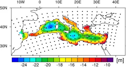
Fig. 1. Topography changes between 9K and CTRL. The superim-posed dots represent 1 of each 10 grid box centre of the model in each direction.
Lamb, 1977). The treatment of subgridscale mixing is done with an isopycnal diffusion scheme; at the surface, a simple mixed layer scheme is included to account for the effect of the wind mixing; in the interior, the Richardson number de-pendant mixing term follows the PP scheme (Pacanowski and Philander, 1981). Convective adjustment is treated by an en-hanced vertical diffusion coefficient for tracers (0.5 m2s−1). The model grid covers the entire Mediterranean Sea includ-ing the Black Sea and a small area of the Atlantic, west of Gibraltar (Fig. 1). The grid is curvilinear with a horizontal resolution of roughly 20 km. We use a 29-level z-coordinates system, with 5 levels within the upper 54 m. The thickness of the first ocean layer is 12 m plus sea level. The model SST is centred at 6 m depth. The time step is 36 min.
The topography is realistic, the Strait of Gibraltar and the Bosphorus are both represented by one grid point and their sills have depths of 256 and 21 m, respectively, in the topog-raphy used for the pre-industrial climate simulation. Dur-ing the early Holocene, the sea level was approximatively 20 m lower than today. To account for this in the paleo-simulations, we reduced the depth by modifying the Mediter-ranean Sea topography according to the ICE-5G reconstruc-tion from Peltier (2004) (Fig. 1). Moreover, we assume the Bosphorus to be closed at this time, so that there is no outflow of fresher water from the Black Sea into the Marmara Sea. We base this assumption on the study from Ryan et al. (1997) who consider a catastrophic inflow of water from Mediter-ranean into Black Sea happening around 8.4 ka BP, and the study from Sperling et al. (2003) who reconstructed high salinities in the Marmara Sea for S1 sapropel time. However, other studies contradict this statement; Aksu et al. (2002), for instance, suggest an overflow from the Black Sea into the Marmara Sea from 10.5 ka BP onwards with low salinities found in the Marmara Sea. A recent study by Soulet et al. (2011) suggests a reconnection at around 9 ka BP.
2.2 Atmospheric forcing and boundary conditions
At the surface, the Mediterranean regional OGCM is forced by air-sea fluxes of heat, momentum and water. The heat fluxes are calculated from daily atmospheric data with bulk formulas according to da Silva et al. (1994).
The atmospheric forcing is derived from long-term simu-lations performed with the coupled global circulation model ECHAM5/MPIOM/LPJ in a global setup (Mikolajewicz et al., 2007). The atmosphere component ECHAM5 (Roeck-ner et al., 2003) has a T31 horizontal resolution and 19 ver-tical levels; the ocean component MPIOM has a curvilinear grid with poles over Greenland and Antarctica. The hori-zontal resolution of MPIOM is roughly 3◦, and there are 40 vertical levels. The dynamical vegetation component LPJ has the same horizontal resolution as the atmosphere component. 2.2.1 Global model setup
The simulations with the global model are carried out until equilibrium for the pre-industrial climate and for two differ-ent simulations of the HIM. The reference simulation refers to a pre-industrial type climate. Following the PMIP2 proto-col (Braconnot et al., 2007), the atmospheric partial pressure of CO2 (pCO2) is set to 280 ppm and the insolation
corre-sponds to 1950 (changes in the orbital parameters lead to negligible insolation differences between 1750 and 1950). For the HIM (9 ka BP), the global simulation used to force the “9K1” regional simulation only considers changes in in-solation. In the HIM global simulation used to force the “9K2” regional simulation, besides the changes in earth or-bital parameters, the atmospheric pCO2 is set to 260 ppm instead of 280 ppm and the topography is modified using ice sheet distributions and topography changes according to the ICE-5G reconstruction (Peltier, 2004).
From these global simulations, we derive three different sets of atmospheric forcing input: one for the pre-industrial climate used as control climate (CTRL) and two for the HIM climate (9K1 and 9K2).
between principal component time series of empirical or-thogonal functions (EOFs, von Storch and Zwiers, 1999) of (i) the anomalies of SLP data from NCEP and (ii) the lies of wind stress data from NCEP. Afterward, SLP anoma-lies from the coarse resolution global model are projected onto the EOFs. Wind stress anomalies are estimated from the obtained loadings using the regression matrix obtained from the NCEP reanalysis. Finally, the wind stress anomalies are added to the long-term mean of NCEP reanalysis data.
As the global model has a cold bias over the Mediter-ranean, the systematic bias between the model and the NCEP climatology is added to the actual model values for near-surface air temperature and dew point temperature.
2.2.2 Freshwater fluxes and restoring
The components of the water fluxes are the monthly pre-scribed river runoff (R), the precipitation (P) from the at-mospheric data derived from the global model, and the evap-oration (E) calculated from the latent heat flux using model SST. For the river discharge, we use a 1-yr monthly climatol-ogy from the UNESCO RivDis database (V¨or¨osmarty et al., 1998). The seasonal cycle is taken into account only for the major rivers (Danube, Nile, Dniepr, Rhone, Po and Ebro). For the Nile and the Ebro rivers, we consider discharge rates prior to the damming, with a yearly averaged runoff of 2930 m3s−1for the Nile and 410 m3s−1for the Ebro. For the HIM simulations, the anomalies (9 K vs. CTRL) of the river discharge simulated by the coupled model are superim-posed on the monthly climatology of river runoff used for the CTRL experiment.
At the surface, there is no restoring to SST and SSS. At the western margin of the Atlantic box, a restoring to climato-logical monthly temperature and salinity from World Ocean Atlas (WOA, Levitus et al., 1998) is applied over 5 grid cells. For the paleo-simulations, the same procedure is applied as for the runoff: the anomalies (9 K vs. CTRL) of the Atlantic hydrography from the global model experiments are super-imposed to the values used in CTRL.
The evaporation is varying, depending on the latent heat flux, which is a function of the SST. As the freshwater fluxes also affect sea level due to the mass flux boundary condi-tion, the net evaporation of the Mediterranean would lead to a continuously decreasing sea level. To account for this, we perform a sea level restoring in the 5 most western grid cells of the Atlantic buffer zone, thus, ensuring that the net water transport through the Strait of Gibraltar corresponds to the net water loss in the Mediterranean and the Black Sea. 2.3 Spin-up and initial conditions
The integration time strongly differs between the already ex-isting studies: 25 yr for Bigg (1994), 20 yr for Meijer and Tuenter (2007), 100 yr for Myers et al. (1998) and Myers and Rohling (2002), 1000 yr for Meijer and Dijkstra (2009) and
1999 yr for Mikolajewicz (2011). A long spinup is essential to reach an ocean state which is no longer drifting from the surface to intermediate depths. We, therefore, perform 700 yr simulations with the Mediterranean OGCM.
We start the three simulations from an initial state with homogeneous low density water (20◦C and 38 g kg−1for the Mediterranean and the Atlantic box; 20◦C and 20 g kg−1for the Black Sea) and let the model run in a free mode for 700 yr, forced by the 100-yr daily atmospheric dataset repeated in a loop. Such initial conditions allow the model to form its own water masses without being under the influence of starting hydrographic conditions derived from a climatology. Because these experiments were started from homogeneous light water and the forcing is not transient, our simulations can only lead to an ocean state with an active deep circula-tion as stacircula-tionary solucircula-tion, because cross-isopycnic mixing would prevent a state with stagnant deep water to be main-tained, through the slow erosion of the stratification.
The results presented in this study correspond to an annual climatology based on the last 100 yr (years 601 to 700).
3 The general features of the Eastern Mediterranean Sea for the control climate
For convenience, Fig. 2 names and locates the sub-basins of the Mediterranean, as well as the main straits.
3.1 Near-surface circulation and deep water formation
The circulation features of the Eastern Mediterranean Sea for the CTRL climate are illustrated in Fig. 3 by the near-surface currents field at 27 m depth. Two intense cyclonic gyres are represented in the Adriatic and in the North Levantine basin (Rhodes Gyre). These gyres correspond to the loca-tion of dense water formaloca-tion. Consistently with the descrip-tion of the horizontal circuladescrip-tion structure summarized by Pinardi and Masetti (2000), the Atlantic-Ionian Stream com-ing from the Atlantic Ocean and entercom-ing through the Strait of Sicily into the central Ionian is well-simulated, as are the Mid-Mediterranean Jet flowing between Crete and the North African coast and the Asia Minor Current flowing along the Turkish coasts.
Linked to this general circulation, the winter mixed layer depth is an indicator widely used to assess the ability of a model to form the different Mediterranean water masses. In our model, the mixed layer depth is a purely diagnosed quantity which is calculated from a density criterion of 0.125 kg m−3, whose value has been originately motivated by the Levitus Atlas (Levitus, 1982). Such a calculation can only give an approximative estimate of the depth of the mixed layer.
Fig. 2. Sub-basins of the Mediterranean: Gulf of Lion (GL), Alboran Sea (ALB), Tyrrhenian Sea (TYR), Adriatic Sea (ADR), Ionian Sea (ION), Aegean Sea (AEG), Levantine Sea (LEV). The Atlantic box (ATL) and the Black Sea (BS) are shown as well. The main straits are marked with a red star.
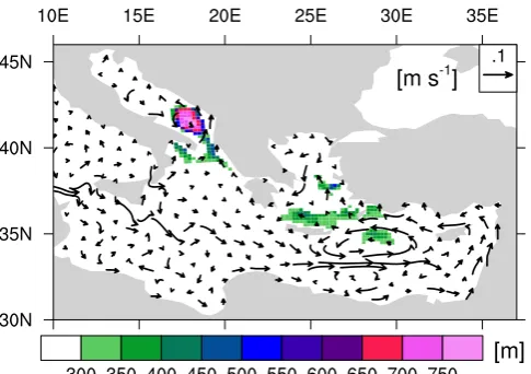
Fig. 3. Modelled March mixed layer depth (colours) and near-surface currents field (arrows) at 27 m depth for CTRL. Only a sub-set of vectors has been plotted. The mixed layer depth is reached when the density difference between this depth and the surface ex-ceeds 0.125 kg m−3. Note that such a calculation can only give an approximative estimate of the depth of the mixed layer.
the South Aegean Sea and in the North Levantine where the Levantine Intermediate Water (LIW) is formed. In the Ionian Sea, the mixing of transformed LIW with out-flowing ABW forms the Eastern Mediterranean Deep Wa-ter (EMDW). The modelled mixed layer patWa-terns are re-alistic and consistent with the climatology of D’Ortenzio et al. (2005) based on observations and calculated with a temperature difference criterion.
The strength of the Mediterranean thermohaline circula-tion (MTHC) is assessed with the zonal overturning stream function displayed in Fig. 4. Driven by salinity and tempera-ture differences, the MTHC is characterised by two main cir-culation cells. The first cell covers both the western and east-ern basin, and has a clockwise circulation with modified At-lantic water travelling toward the east at the surface, and LIW travelling from the east to the west at intermediate depth. A maximum of 1.1 Sv is found at subsurface depth, between
Fig. 4. Zonal overturning stream function integrated over the entire Mediterranean basin for the CTRL experiment. It has been calcu-lated on the basis of a 100-yr mean velocity field.
100 and 200 m depth. Located in the eastern basin, the sec-ond cell shows a counterclockwise vertical circulation which is much weaker with a maximum of 0.2 Sv. This cell corre-sponds to the circulation of EMDW toward the extreme east of the basin, this being compensated by a subsurface flow of LIW from the Northern Levantine toward the west.
The model simulates an averaged net water transport at Gibraltar of 0.051 Sv (1 Sv = 106m3s−1), with a surface
Fig. 5. Annual, winter (JFM) and summer (JAS) SSTs at 6 m depth for CTRL (left), World Ocean Atlas 1998 climatology (middle) and MEDATLAS climatology (right).
3.2 Surface temperature and salinity
To assess the ability of the model to reproduce observed SST and SSS patterns, we compare our results from the CTRL simulation with the climatologies from WOA 1998 (Levi-tus et al., 1998) and MEDATLAS (MEDAR-Group, 2002). Because the temperature point in our model vertical dis-cretization is at 6 m depth, we consider the climatological temperature interpolated to 6 m depth to make a consistent comparison.
Figure 5 shows the comparison between the modelled and both climatological SSTs. The model exhibits SST gradient from west to east and from north to south, consistently with the climatologies. For the annual mean as well as for win-ter (JFM) SSTs, the deviations remain below 1 K. The winwin-ter modelled SST values are in between the values of both cli-matologies, MEDATLAS showing slightly warmer SST than WOA in the Levantine Sea and in the southern Ionian Sea. Both the Aegean and Adriatic Seas have too cold simulated temperatures during winter time. These regions are almost land-locked, with narrow connections to the wider part of the Eastern Mediterranean, through the Strait of Otranto for the Adriatic Sea and three straits of the Cretan Arc for the Aegean Sea. Small-scale atmospheric processes are acting over both areas, so that accurate wind patterns are difficult to simulate adequately at the resolution we are using. For
summer (JAS), WOA displays SST 1 to 2 K warmer than MEDATLAS. The modelled summer SST shows warm bi-ases in comparison with both climatologies. In the southern Ionian Sea and in the eastern Levantine Sea, biases up to 3 K are simulated by the model (in comparison with MEDAT-LAS, the coldest climatology). These biases could be due to the Atlantic-Ionian jet travelling slightly too far north in the model (compared to Pinardi and Masetti, 2000), thus, reduc-ing the import of cooler water from the western basin into the southern Ionian Sea.
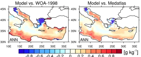
Fig. 6. Annual mean SSS deviations at 6 m depth. CTRL vs. World Ocean Atlas 1998 climatology (left) and CTRL vs. MEDATLAS climatology (right) are represented.
observational data, which has been introduced in the gener-ation of the observgener-ational climatologies. Finally, the model has a positive salinity bias all along the North African coast. There are several contributors to this bias. First, this area has a warm SST bias (probably linked to the inability of the model to represent small scale atmospheric processes at the coasts, as explained before), this leads to a stronger evapora-tion and consequently higher salinities. Second, the regional river discharge may be underestimated. Third, the Atlantic-Ionian jet, which brings fresher water to the eastern basin, is located slightly too far north in the model. Thus, the south-ern Ionian remains somewhat isolated and is not significantly impacted by this fresher current. Most of the discrepancies do not reflect the inadequacy of the model to correctly sim-ulate consistent SSS, but they can be directly linked to some discrepancies in the freshwater components of our forcing, mainly the too low precipitation (explained hereafter) as well as missing river discharge. On average, this induces a mean positive salinity bias of 0.25 g kg−1in the eastern basin. 3.3 Water budget
Table 1 summarizes the different components of the freshwa-ter budget for the Medifreshwa-terranean. The averaged precipitation prescribed over the Mediterranean Sea from the global model is only 0.59 mm d−1and the averaged calculated evaporation is 2.83 mm d−1. The rivers contribute to the freshwater input by adding 0.35 mm d−1. The input from the rivers is close to the data from Ludwig et al. (2009), who indicate a value of 0.39 mm d−1. Nevertheless, the amount of prescribed pre-cipitation is relatively low in comparison with both obser-vations and reanalysis (0.7 mm d−1 in HOAPS, Andersson et al. (2007); and 1.07 mm d−1in ERA-Interim Reanalysis, Simmons et al. (2007)). The interactively calculated evapo-ration is also lower than values from reanalysis (3.34 mm d−1 in ERA-Interim Reanalysis) and observations (3.12 mm d−1 in HOAPS).
The resulting water deficit of 1.89 mm d−1is compensated by the positive net freshwater transport from the Black Sea into the Mediterranean through the Strait of the Dardanelles (0.18 mm d−1 or 0.0055 Sv) and from the Atlantic Ocean through the Strait of Gibraltar (1.71 mm d−1 or 0.051 Sv).
The net water transport through both straits is consistent with the observations. Bryden et al. (1994), Bryden and Kinder (1991) and B´ethoux (1979) suggest the values of 1.42 mm d−1, 1.37–1.64 mm d−1 and 2.74 mm d−1, respec-tively, for the estimation of the net water transport at Gibral-tar. Concerning the net water transport from the Black Sea through the Strait of the Dardanelles, the data from Stanev and Peneva (2002) indicate a value of 0.22 mm d−1.
In Table 1, we also compare the mean values of each com-ponent of the water budget averaged for the full Mediter-ranean with those averaged for the eastern basin only (from the Strait of Sicily until the Bosphorus). This shows how much the eastern basin differs from the western in terms of
E-P balance. We observe that the mean precipitation rate in the eastern basin is around 20 % lower than for the full basin, the mean river input is 6 % lower and the mean evaporation is 6 % higher. The Nile is responsible for 44 % of the river input of the eastern basin.
4 The Holocene Insolation Maximum
4.1 Stronger seasonal cycle
In the HIM global simulations, the changes in the Earth’s or-bital parameters lead to stronger amplitude of the seasonal cycle of insolation. The averaged downward short wave ra-diation at the top of the atmosphere over the Mediterranean Sea is increased by about 15 W m−2during the summer sea-son and is decreased by about 15.5 W m−2 during the
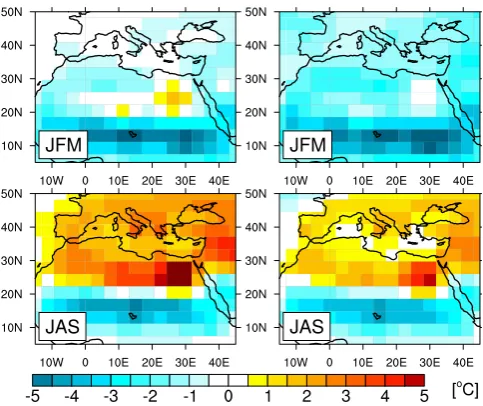
win-ter season for both 9K1 and 9K2 experiments in comparison with the CTRL experiment. This leads to an increased sum-mer warming and an enhanced winter cooling as shown by the near-surface air temperature anomalies signal displayed in Fig. 7. The more realistic set up in 9K2, with the de-caying Laurentide ice sheet and lower atmospheric pCO2, leads to a generally slightly colder climate than in 9K1. In 9K2, the summer warming is smaller and the winter cooling is stronger compared to the 9K1 simulation.
Table 1. Freshwater budget for the Mediterranean and the Eastern Mediterranean for CTRL, 9K1 and 9K2.
Mediterranean Eastern Mediterranean
[mm d−1] CTRL 9K1 9K2 CTRL 9K1 9K2
Precipitation (P) 0.59 0.66 0.60 0.51 0.58 0.52 Evaporation (E) 2.83 2.87 2.83 2.99 3.03 2.98 River runoff (R) 0.35 0.53 0.45 0.33 0.61 0.49
P+R-E −1.89 −1.68 −1.78 −2.15 −1.84 −1.97 Net water transport 1.71 1.68 1.78
at Gibraltar
Net water transport 0.18 0.28
at Bosphorus
[m3s−1]
River runoff (R) 10 443 15 535 13 070 6630 11697 9319
Nile runoff 2930 7494 5401 2930 7494 5401
Net water transport 51 000 49 000 52 000 at Gibraltar
Net water transport 5621 5621
at Bosphorus
Fig. 7. Anomalies of 2-meter air temperature for winter (JFM) and summer (JAS) from global simulations, 9K1 vs. CTRL (left) and 9K2 vs. CTRL (right).
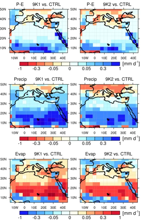
positiveP-Eanomalies) in both simulations (Fig. 8). The Nile has a larger water discharge for the HIM with runoff sur-plus of 4564 m3s−1for the 9K1 simulation and 2471 m3s−1 for the 9K2 simulation compared to the CTRL experiment.
Fig. 8. Annual mean anomalies ofP-E,P andEfrom global sim-ulations, 9K1 vs. CTRL (left) and 9K2 vs. CTRL (right).
In general, the freshwater budget does not show strong changes because the enhanced Nile runoff partially compen-sates the missing water from the Black Sea.
4.2 Salinity, stratification and deep water formation
As a consequence of the missing outflow from the Black Sea due to the closure of the Bosphorus in the HIM simu-lations, the salinity of the Aegean Sea increases in 9K1 and 9K2 (Fig. 9). This results in a shift of the location of in-termediate water formation from the North Levantine/South Aegean towards the North Aegean (Fig. 9). This confirms what has been recently suggested by the proxy-based study of Schmiedl et al. (2010), which implies a persistent deep wa-ter ventilation in the northern Aegean Sea during the HIM. In our simulations, the salty and relatively dense water formed in this region flows out of the Aegean Sea through the Strait of Antikithira and follows the western Greek coast towards the Adriatic. Along the trajectory following western Greece,
Fig. 9. Annual mean SSS (CTRL, top) and SSS anomalies vs. CTRL (9K1, middle; 9K2, bottom) at 6 m depth (colours). March mixed layer depth is overlaid as fill patterns.
a mixed layer pattern of intermediate depth appears due to the fact that the dense salty water flowing from the Aegean entrains the surrounding lighter water on its way to the Adri-atic. During the HIM, the deep outflow of Mediterranean water through the Strait of Gibraltar decreases with values of 0.72 and 0.77 Sv, respectively, for 9K1 and 9K2 (vs. 0.79 Sv in CTRL).
simulation has a lower sea level, which is not the case in the 9K1 global simulation. Acting in the opposite direction, the enhanced discharge of the Nile tends to reduce the salinity. The latter effect is stronger in 9K1 than in 9K2. Despite their differences in SSS anomalies, the modelled winter mixed layer depth patterns remain similar in both HIM simulations. The simulated SSS anomalies display a signal which is not too far from the one reconstructed for 9 ka BP. In the Tyrrhe-nian Sea, Kallel et al. (1997) reconstructed SSS around 1 g kg−1 saltier than today, the model simulates positive anomalies of 0.1 (9K1) and 0.35 g kg−1 (9K2). In the Io-nian Sea, Emeis et al. (2000) reconstructed SSS anomalies 1 g kg−1 higher than present-day, the model exhibits SSS anomalies of + 0.35 (9K1) and + 0.5 g kg−1(9K2). Finally the SSS signal reconstructed in the Levantine by Emeis et al. (2000) is 2 g kg−1 fresher than today, whereas the model
shows SSS anomalies of - 0.15 (9K1) and + 0.2 g kg−1(9K2).
The inconsistency between model and reconstruction in the Levantine is probably related to the Nile runoff which could be underestimated by the global model (particularly in the 9K2 simulation), thus leading to too salty SSS.
To assess the impact of the salinity changes on the venti-lation of the deeper layers, we focus on the vertical stratifi-cation of the water column and calculate an Index of Strati-fication (IS) (in m2s−2, see Beuvier et al., 2010; ?; Somot, 2005; Lascaratos, 1993). This index has been used in previ-ous studies to investigate the preconditioning of the convec-tion by looking at the changes in the vertical stratificaconvec-tion. It corresponds to the loss of buoyancy required to induce a convection event up to the bottom of the sea. The lower the index, the more likely the convection to occur is. IS is calcu-lated on a 100-yr mean basis, for each model grid point (i,j) using the following formula:
IS(i,j,hbot)= Z hbot
0
N2(i,j,z) z dz, (1) wherezis the depth,hbotis the depth at the bottom andNis the local Brunt-Vaisala frequency:N2=g
ρ ∂ρ ∂z.
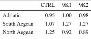
Table 2 compiles IS values averaged over the main convec-tive areas for the three simulations. In the Adriatic, the most active location for deep water formation, low IS values are displayed for the three simulations, reflecting a weak stratifi-cation. From these similarities, we infer that the deep water production in the Adriatic remains identical during the HIM with formation rates comparable to CTRL. This happens be-cause the changes in surface salinity have reached the deeper layers and the state has became quasi-stationary with a stable density gradient similar to CTRL. During the HIM, both past experiments simulate a decreased IS in the North Aegean and an increased IS in the South Aegean in comparison with CTRL, consistently with the shift of winter mixed layer depth pattern from the south to the north displayed in Fig. 9.
We, thus, obtain 3 simulations, each representing a well-ventilated state. Winter convection occurs in different sub-basins to form intermediate and deep water. Dense water
Table 2. Index of Stratification (IS, in m2s−2).
CTRL 9K1 9K2
Adriatic 0.95 1.00 0.98
South Aegean 1.07 1.27 1.27 North Aegean 1.25 0.92 0.89
formation takes place in the Adriatic, the South Aegean and the Northeastern Levantine in CTRL. In the HIM simula-tions, dense waters are formed in the Adriatic and the North Aegean. Despite these small shifts of winter mixed layer depth patterns between past and present, the HIM zonal over-turning stream function remains almost identical, with a deep counter-clockwise cell in the eastern Mediterranean, display-ing a maximum value of 0.2 Sv, as seen in CTRL (Fig. 4). These simulated past climate states aim at representing a stable and stationary environment before entering into the transition phase which triggered the sapropels through weak-ened/prevented ventilation of the deep water.
4.3 The upper-ocean temperature
4.3.1 Seasonal cycle
As a direct effect of the changes in incoming short wave ra-diation at the surface, an increase in the amplitude of the sea-sonal cycle of the water temperature (Fig. 10) is simulated. The enhanced cooling during winter spreads over the entire water column through mixing and convective processes. The enhanced seasonal cycle leads to warmer surface tempera-tures in both 9K simulations in summer. During spring and summer, stable stratification prevents a deep penetration of the warming signal. The region with temperatures warmer than in the CTRL run is, thus, restricted to the upper 30 and 20 m, respectively, for the 9K1 and 9K2 simulations. Be-cause the 9K1 simulation is generally warmer than the 9K2 simulation (the latter being colder due to the presence of rest of the Laurentide ice sheet and reduced atmosphericpCO2in 9K2), the summer warming relative to the CTRL run is more pronounced (up to 1.5 K for the surface water of the 9K1 ex-periment vs. 0.8 K for 9K2) and spreads slightly deeper than for the 9K2. Below, the water shows cold anomalies during summer, which is a remainder from the cold winter signal. 4.3.2 The western Levantine subsurface warming
pattern
Fig. 10. Anomalies in monthly seasonal cycle of upper ocean tem-perature averaged over the Eastern Mediterranean, 9K1 vs. CTRL (left) and 9K2 vs. CTRL (right); isolines represent the absolute val-ues in◦C for 9K1 (left) and 9K2 (right).
Fig. 11. Anomalies of summer (JAS) temperature at different depth levels, 9K1 vs. CTRL (left column) and 9K2 vs. CTRL (right column).
anomaly signal shows strong regional contrasts with a well-defined pattern. At a 17 m depth, the region around Crete and the western Levantine still show a warming signal, whereas the central Ionian, the Tyrrhenian and, only for 9K1, the eastern Levantine, experience a cooling. At a 27 m depth, cooling is mainly observed over the Eastern Mediterranean, but is strongly reduced around Crete and western Levantine, and even absent in the 9K1 simulation.
The pattern of subsurface temperature anomalies is quite similar to the present-day pattern of subsurface spread of the summer SST in the Eastern Mediterranean (Fig. 12). The model shows weaker vertical gradients of the near-surface
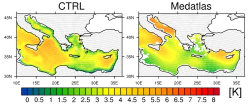
Fig. 12. Summer (JAS) temperature difference between 6 and 27 m of depth, for CTRL and MEDATLAS climatology.
temperature in the western Levantine (and, thus, a deeper penetration of the summer warming signal) than in the east-ern Levantine and the Ionian; the same patteast-ern is also obvious in the MEDATLAS climatology.
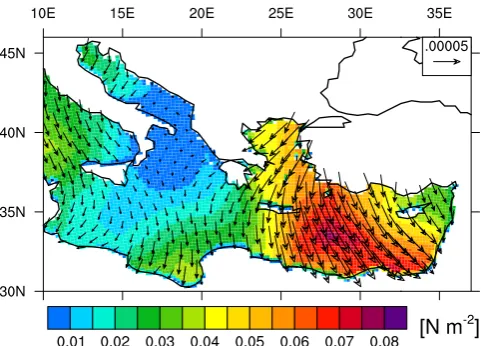
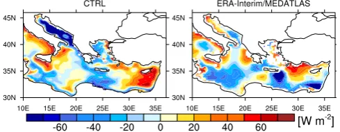
The reduced vertical near-surface temperature gradient in the western Levantine is caused by the Etesian winds. The Etesian winds are dry northerly winds blowing over the Aegean Sea and the Levantine Sea from about mid-May to mid-September, mainly because of the monsoon effect lead-ing to a thermal low pressure trough over Turkey, with higher pressure over southern Balkans; and the passage of cold fronts over the Balkans and the associated cold-air circula-tion behind them (e.g. Meteorological-Office, 1962; Brody and Nestor, 1985). In the model derived forcing used for CTRL, Etesian winds are acting from May until mid-October (Fig. 13, black line) and are essentially a north-south blowing wind (Figs. 13 and 14). The westward Ekman trans-port induced by this wind pattern involves the upwelling of cold subsurface water in the eastern Levantine (resulting in a strong vertical near-surface temperature gradient) and down-welling of warm surface water west of the core of the Etesian winds with a reduced vertical near-surface temperature gradi-ent. As an example, the vertical velocities and the associated subsurface heating rates are displayed in Fig. 15. The west-ward Ekman transport leads to a substantial heat transport from the eastern to the western Levantine. This becomes evi-dent when comparing the atmospheric heat input with the ac-tually observed changes in ocean heat content for the period from May to September, when the Etesian winds are present (Fig. 16, left). In the western Levantine, an additional heat source of up to 60 W m−2working for 5 months is required to explain the changes in ocean temperature. In the eastern Levantine, a similar heat sink is required (up to 65 W m−2).
(Fig. S1 in the Supplement), indicating that the heat “piracy” of the western Levantine is restricted to late spring and sum-mer. In the other months of the year, the western Levantine is actually exporting heat.
In order to determine, whether the summer heat piracy is a model artefact, we performed the same calculation using net atmospheric heat input from the ERA-Interim Reanalysis averaged over the years 1989–2005 (Berrisford et al., 2009) and the ocean heat content changes calculated from the ME-DATLAS temperatures (Fig. 16, right). The results show an even stronger heat piracy (up to 150 W m−2) around Crete and in the southeastern Levantine. Additional simulations performed with our ocean model forced with ERA-Interim derived atmospheric forcing have produced similar results (not shown). The difference between modelled and observa-tion derived-estimates can be explained by differences in the Etesian winds. The Etesian winds derived from the global model are essentially blowing from the north (Figs. 13 and 14). In the present-day observations, they also have a erly component over the Levantine, thus, causing the west-east dipole of the model to be somewhat rotated with the strongest part of the upwelling shifted more to the southeast, and the strongest part of the downwelling shifted more to the south. The observed Etesian winds are also slightly stronger, which explains the stronger heat piracy in the observation-based estimate.
During the HIM, the amplified seasonal cycle of surface temperature (which is a direct effect of the insolation forcing) enhances the vertical gradients in near-surface ocean tem-perature. Together with the Ekman-induced circulation, this stronger seasonality of the insolation cycle could explain the pattern of subsurface temperature changes displayed by the anomalies 9K vs. CTRL (Fig. 11). In the upwelling region of eastern Levantine, colder subsurface water is upwelled, in the western Levantine warmer surface water is downwelled, thus, causing a positive anomaly of subsurface temperatures. Additionally, the modelled Etesian winds are found to be increased for both HIM experiments (Fig. 13): a further strengthening of the temperature dipole is, thus, expected through enhanced Ekman transport.
In the following, the respective contributions of increased Etesian winds and enhanced seasonal cycle of insolation, to the subsurface temperature anomaly in the Cretan and south Levantine regions are analysed. For this purpose, two differ-ent 100-yr sensitivity experimdiffer-ents are set up, all starting in year 600 of experiment 9K2:
- 9K2-W0 uses the same setup as the 9K2 simulation, but both wind speed and wind stress from CTRL (weaker Etesian winds) are prescribed. With this simulation, the effect from the “full” wind (speed and stress) on the 9K2 climate can be assessed when compared with 9K2, and the effect of the increased thermal forcing alone can be assessed when compared to CTRL.
- CTRL-W9 is similar to CTRL simulation, but we pre-scribe both wind speed and wind stress from the 9K2 experiment (enhanced Etesian winds). This simulation enlightens the effect of the “full” wind signal (speed and stress) on the CTRL climate when compared with CTRL.
Figure 17 displays the contribution of different factors to temperature anomalies at different levels of the subsur-face. Factors analysed are (i) the enhanced insolation forc-ing (9K2-W0 vs. CTRL), (ii) the increased Etesian winds on CTRL climate (CTRL-W9 vs. CTRL), and (iii) the increased Etesian winds on 9K2 climate (9K2 vs. 9K2-W0). Sepa-rate contributions are compared to the total effect from both increased winds and enhanced seasonal cycle of insolation (9K2 vs. CTRL).
The pure effect of the insolation in the 9K2 simulation is dominant in the first model layer (0–12 m), and is responsi-ble for a mean warming of 0.5 K (Fig. 17a). The contribu-tion of enhanced winds induces a mean cold bias of 0.3 K on a CTRL climate (Fig. 17b) and 0.2 K on a 9K2 climate (Fig. 17c). The wind-induced cooling is almost entirely a consequence of the enhanced wind speed which induces a stronger mixing at the top of the water column; this leads to stronger heat transfer from the sea surface toward subsur-face, explaining the cold anomalies in the first ocean layer. The wind stress effect is small at the surface.
In the second layer (12–22 m), the insolation effect is strongly reduced with a warming around 0.2 K in the Cretan and southwestern Levantine regions and a cooling in east-ern Levantine (Fig. 17e). These patteast-erns are expected in this case, which combines enhanced summer insolation sig-nal and present-day winds: the water downwelled in south-western Levantine is warmer, leading to warmer pattern, and the subsurface water upwelled in eastern Levantine is colder, leading to cooler pattern. In this second layer, the main ef-fect of stronger Etesian winds is still a cooling (Fig. 17f and 17g), however, a warming up to 0.2 K becomes noticeable in the south Levantine area on 9K2 climate (Fig. 17g).
Fig. 13. Monthly climatology of wind components averaged over the Aegean/West Levantine regions for CTRL (black), 9K1 (blue) and 9K2 (red). Left panel shows 10-m wind speed cubed, the cubed value is considered because it is proportional to mixing strength. Right panel shows both west-east and north-south wind stress components. The shading represents the time period, when modelled Etesian winds are active.
Fig. 14. Mean summer (JAS) wind stress for CTRL.
speed is responsible for warm anomalies southeast of Crete in the layer 22–32 m, where heat is gained through higher transfer to subsurface.
In general the wind effects become stronger when acting on a temperature distribution with enhanced vertical gradi-ents. This becomes obvious when comparing the respective panels with wind effects on CTRL and 9K2 basis state. Thus, the nonlinear effects between the two mechanisms (stronger seasonal cycle and stronger Etesian winds) are amplifying the temperature signal.
When all effects are combined, the total results to a subsur-face warming pattern around Crete and in southwestern Lev-antine in the 12–22 layer (Fig. 17h). The warming around Crete vanishes for the 22–32 m layer (Fig. 17l), because of the prevailing cooling from the insolation signal (Fig. 17i).
Fig. 15. Temperature change through vertical advection averaged between 12 and 42 m of depth (colours) and vertical velocities (fill patterns, positive values for upward velocities) in July for CTRL.
Only the warming in southwestern Levantine (induced by enhanced downwelling of warm water) is strong enough to prevail in the layer 22–32 m (Fig. 17l).
Fig. 16. Difference between the net atmospheric heat input and changes in ocean heat content from 1 May until 30 September. Left panel shows CTRL. Right panel shows differences between net at-mospheric heat input from ERA-Interim Reanalysis (averaged over 1989/2005) and changes in ocean heat content from MEDATLAS climatology. Positive values indicate that the atmospheric input is higher than the temperature change in the water column, reflecting an export of heat from this region. Negative values reflect a heat accumulation.
4.4 Comparison to proxy data
4.4.1 The SST reconstructions
The transfer function used to reconstruct the paleo-SST is based on census counts of 23 species of planktonic foraminiferal species in 274 core tops, 145 from the Mediter-ranean and 129 from the Atlantic (Hayes et al., 2005). The data are calibrated to seasonal (JFM and JAS) and annual mean SST values at 10 m water depth from the observational dataset WOA (Levitus et al., 1998). The transfer function method based on “artificial neural networks” is described in Hayes et al. (2005).
Based on14C data, oxygen isotope stratigraphy, biostratig-raphy or a combination of those, the Holocene Insolation Maximum interval has been identified in 33 Mediterranean sediment cores as an interval between approximately 9.5 and 8.5 ka BP. Only samples occurring within this interval, as identified by the individual age models, were considered. Faunal counts were collated with the same procedure as for the core-top samples. SST reconstructions were averaged throughout each Holocene Insolation Maximum Interval for each core.
The full data and discussion of the proxy resulted are pre-sented in a companion paper by Kucera et al. (2011). 4.4.2 SST model-proxy comparison
In this section, we compare the SST modelled in 9K1 and 9K2 with the SST reconstructed from foraminifera for 9.5– 8.5 ka BP. We first consider absolute values and analyse an-nual, summer (JAS) and winter (JFM) temperatures.
Figure 18 displays, for each experiment, the fit between the SST reconstructions and the modelled SST at each core location; for annual mean, winter (JFM) and summer (JAS). In general, the 9K1 simulation, which only considers the
change in solar forcing, yields too warm SST in comparison with the reconstructions. In contrast, the SST predicted by the model in the 9K2 simulation show a better match with the reconstructions because the 9K2 simulation also takes into account the cooling effect of the glaciers and the reduced at-mospheric CO2concentration, which lead to SST around 1 K
colder than for the 9K1 simulation. The model-data discrep-ancies of the 9K1 simulation are mainly located in the central Ionian, with a warm SST bias of 1 K for annual mean and 3 K for summer (Fig. S2 in the Supplement). As for the CTRL simulation, this bias may be linked to the Atlantic-Ionian jet travelling too far north in the model.
The two strongest deviations displayed in Fig. 18 refer to data located in the Adriatic and in the Aegean (Fig. S2 in the Supplement). These two regions are difficult to simulate at our resolution due to their size and small-scale processes act-ing over these areas, among these are katabatic winds, which are not resolved adequately by the coarse global model. This may explain the strong disagreement encountered in these locations with discrepancies up to 6 K and 5 K in summer, respectively, for 9K1 and 9K2 (Fig. S2 in the Supplement). Furthermore, the two temperature reconstructions available for the Adriatic differ strongly so that it is difficult to extract a clear signal from the observations for this region. For the two simulations, the modelled SST fall between both recon-structed SST values. The simulated winter SST matches well with the reconstructed signal (Fig. 18, blue): the biases do not exceed 1 K except for the Aegean. The major disagreement between model and proxy data is restricted to summer SST (Fig. 18, red): both HIM experiments show a warm bias with summer SST errors in excess of 3 K in average for the 9K1 simulation and 2 K for the 9K2 simulation. Again, except for the enclosed Aegean and Adriatic Seas, the major discrepan-cies are found in the central Ionian and in the Tyrrhenian Sea (Fig. S2 in the Supplement).
Fig. 17. Anomalies of temperature for different model depth layers for summer (JAS). The columns show the isolated effect of insolation forcing (9K2-W0 vs. CTRL), enhanced Etesian winds on CTRL climate (CTRL-W9 vs. CTRL) and on 9K2 climate (9K2 vs. 9K2-W0), as well as the total effect of both factors (9K2 vs. CTRL).
Fig. 18. Comparison of modelled SST with SST reconstructed from proxy data (Kucera et al., 2011) for 9K1 (left) and 9K2 (right). An-nual mean, winter (JFM) and summer (JAS) are considered.
signal dampens the stronger summer signal and explains the smoother gradient of the reconstructed annual SST anoma-lies. Concerning the model ability to reproduce these spatial anomaly patterns, the model results are not consistent with the reconstructions. Whereas the tripole pattern is somewhat imaged by the 9K1 simulation for the annual SST anomalies, the 9K2 simulation is again consistently too cold. For the summer SST anomalies, the 9K1 experiment shows a rather homogeneous warming, but hardly any cooling of the mid-dle Ionian and the Tyrrhenian. The 9K2 experiment shows a
much weaker warming and is able to reproduce an enhanced warming pattern around Crete. The modelled winter SST anomalies do not show the warming around Sicily, and the 9K2 experiment simulates a far too strong cooling over the entire basin.
Two points are important to notice at this stage of the analysis: the simulated temperature signal decreases very strongly with depth in the upper part of the water column during the summer season, due to strong stratification (Fig. 10). Moreover, the foraminifera used for the SST recon-structions are not limited to the 10-m depth of the calibration, but inhabit the entire mixed layer and some live even below it (B´e et al., 1977; Schiebel and Hemleben, 2005). They are, thus, likely to record subsurface temperatures as well, which are colder than the surface temperature in summer.
Fig. 19. Annual, winter (JFM) and summer (JAS) SST anomalies, reconstructed from proxy data (dots, Kucera et al. (2011)) vs. mod-elled one (background colour) for 9K1 vs. CTRL (left) and 9K2 vs. CTRL (right). 1st row displays annual SST anomalies, 2nd row displays winter SST anomalies, 3rd row displays summer SST anomalies.
Fig. 20. Comparison of modelledT0−30withT0−30reconstructed from proxy data (Kucera et al., 2011) for 9K1 (left) and 9K2 (right). Annual mean, winter (JFM) and summer (JAS) are considered.
4.4.3 A depth-integrated approach for model-proxy comparison of upper-ocean temperature
In this section, we propose an alternative approach to per-form a comparison of surface temperature signal between output from model simulations and reconstructions based on planktonic foraminifera.
We consider temperatures averaged over a larger depth in-terval for our model-proxy comparison instead of restricting it to a narrowly defined SST signal. As an example, we
Fig. 21. Annual and summer (JAS)T0−30 anomalies, calculated from SST reconstructions from proxy data (triangles, Kucera et al. (2011)) vs. modelled one (background colour) for 9K1 vs. CTRL (left) and 9K2 vs. CTRL (right). 1st row displays annualT0−30 anomalies, 2nd row displays summerT0−30anomalies.
choose to integrate the temperature over the depth interval between 0 and 30 m (henceforthT0−30), where the vertical
temperature gradient is strongest. We do not claim that 0– 30 m is the range of depth which should always be chosen, but we rather aim to highlight the need to consider a broader interval of depth which depends on the living depth of the foraminifera. The interval of depth chosen to integrate the temperature signal should be informed by the oceanographic conditions of a given region and the ecology of the planktonic species used.
The proxy temperatures are, in a strict sense, only valid for 10 m depth. As for many of the core locations, no core top estimates of the pre-industrial climate are available, anoma-lies versus climatologies for this depth have been used. How-ever, this approach is not adequate in obtaining reconstructed anomalies of T0−30 signal: the present-day climatology for T0−30 can easily be calculated from the same climatology,
but the proxy data should have been estimated withT0−30as
the base too, which is beyond the scope of this paper. As a simple approximation, we calculate a linear regression be-tweenT10, which has been originally used to fit the proxy data, andT0−30 from the World Ocean Atlas dataset. Only
data from the Mediterranean and the North Atlantic are used for this calculation (box selected between 30◦and 50◦north and−20◦and 37◦east). We apply this relation to the recon-structed data and get a new set of reconstructions forT0−30.
The functions applied are the following:T0−30=0.97T10 +
0.29 for annual temperatures,T0−30=0.99T10 +0.015 for
winter andT0−30=0.9 T10 +1.45 for summer. The R2
is higher than 0.977 for all three scalings. The root mean square deviation (RMSD) of the obtainedT0−30is 0.41 K for
Table 3. Mean error and mean biases [K].
SST T0−30
9K1 9K2 9K1 9K2
Annual mean Error (RMSD) 1.46 1.04 1.11 1.10 Mean bias 1.02 0.19 0.35 −0.38
Winter (JFM) Error (RMSD) 1.03 1.20 1.03 1.23 Mean bias 0.00 −0.66 0.00 −0.71
Summer (JAS) Error (RMSD) 3.10 2.16 1.83 1.34
Mean bias 2.81 1.73 1.29 0.50
Averaged Error (RMSD) 2.06 1.55 1.37 1.23
Mean bias 1.27 0.42 0.55 −0.59
and the vertical temperature gradient is small. For this sea-son, the results forT0−30are not substantially different from
the results forT10. Thus, the discussion will rather focus on
summer and annual mean.
The new model-proxy comparison for the absoluteT0−30
is displayed in Fig. 20. It exhibits the fit between the re-constructions and the model data at each core location; for annual mean, winter (JFM) and summer (JAS). The new comparison shows a great improvement, especially for the summer season, when the strongest discrepancies were found in the previous strict SST comparison (Fig. 18). For both simulations, the biases between modelled and reconstructed
T0−30 are generally below ±1 K, except for the data
lo-cated in the Adriatic and in the Aegean Seas (Fig. S3 in the Supplement).
Figure 21 displays the new comparison for the T0−30
anomalies (9 ka BP vs. CTRL) simulated by the model and recorded by the proxy indicators. The reconstructed summer
T0−30 anomalies do show the west-east tripole (Fig. 21, 2nd
row). However, in the Tyrrhenian, the central Ionian and the eastern Levantine, the cooling signal is less pronounced than with the strict SST reconstructions; this is in agreement with the modelled signal of the 9K2 simulation. The cold anoma-lies simulated by 9K1 in these regions are weak and even missing for the eastern Levantine. The newT0−30
recon-structions show a more homogeneous warming around Crete. This warming is simulated in the 9K1 experiment, but the warmest anomalies are located in the southwestern Levan-tine. The 9K2 experiment displays a very weak cooling in the Cretan region and a moderate warming in the southwestern Levantine. The model produces the warmest anomalies in the southwestern Levantine rather than in the Cretan region because the downwelling of warm surface water is simulated too far south. Nevertheless, in few locations, the anomalies (9 ka BP vs. present-day) of estimatedT0−30reconstructions
show a signal which is lower than the RMSD of the estimated summerT0−30signal (0.41 K). These results should, thus, be
interpreted cautiously.
It is worth mentioning that if the modelled Etesian winds had a stronger westerly component, and had their core cen-tred over the east Aegean (as it is recorded by the ob-servations), the downwelling of warm surface water would occur around Crete, leading to warm subsurface anoma-lies there rather than in the southwestern Levantine (as shown in Fig. 16, right). This would also improve the agreement between model and proxies, showing a modelled warming more centred around Crete, consistently with the reconstructed signal.
To summarize the results from the model-proxy compar-ison and to highlight the added value from the novel inte-grated approach, Table 3 compiles the mean bias and the mean standard error (RMSD) for (i) the SST comparison and (ii) theT0−30 comparison. The most obvious improvement
is for summer, when both 9K1 and 9K2 simulations reach a much lower mean bias with the T0−30 comparison. The
RMSD is also clearly improved. As expected, there is hardly any difference between the SST andT0−30 comparisons for
winter, because the small temperature gradient during this season leads to similar results. If we average the mean bias and the RMSD for the three considered periods (winter, sum-mer and annual mean), it is clear that theT0−30 comparison
leads to a better match. In our point-of-view, the experiment 9K2 fits the reconstructions the best. Although the mean bias is slightly higher than for 9K1 (−0.59 K vs. 0.55 K), the RMSD value of 9K2 is lower (1.23 K vs. 1.37 K).
These results confirm the hypothesis that the model-proxy comparison should involve a temperature signal integrated over a wider range of subsurface depth, consistent with the range of living depths of the planktonic foraminifera used, in-stead of restricting the comparison to the SST. Ideally, a new transfer function should be used to perform the reconstruc-tions, taking into account an integrated temperature signal whose depth range should be previously determined.
fact that the forcing used for this simulation does neither in-clude the cooling effect from the melting glaciers nor from the lowerpCO2.
5 Conclusions
We have modelled the upper ocean climate of the East-ern Mediterranean for the Holocene Insolation Maximum (9 ka BP) with a regional OGCM forced by daily atmospheric data derived from global simulations. Two experiments have been carried out: 9K1 with changes in solar forcing only and 9K2 with changes in solar forcing, atmosphericpCO2 and topography (presence of major ice sheets).
We analysed the mechanisms responsible for the enhanced subsurface summer warming observed in the Cretan/West Levantine region during the HIM, which is recorded by both the model and proxy data. The drivers of this warming are found to be a combination of (i) enhanced downwelling (due to stronger Ekman transport) and wind mixing, both due to strengthened Etesian winds, and (ii) enhanced vertical tem-perature gradient due to the stronger seasonal cycle in the Northern Hemisphere. Together, these processes induce a stronger heat transfer from the surface to the subsurface dur-ing late summer in the western Levantine and are responsible for the heat piracy simulated in this region.
We used SST reconstructed from planktonic foraminifera assemblages to validate our HIM simulations, but found it necessary to integrate modelled SST over a wider depth range to account for variable habitat depth. We believe that this is how surface temperature comparisons between model data and reconstructions from foraminifera should be per-formed. This novel depth-integrated approach strongly im-proved the agreement between the reconstructions and the modelling results. The currently used technique to recon-struct temperature from planktonic foraminifera is likely in-adequate for time periods when the vertical temperature gra-dient was different from today, which is likely to have been the case in the isolated Mediterranean Sea for periods with changing insolation. Ideally, the transfer function should be newly calculated for the temperature integrated over the con-sidered depth range including subsurface.
We believe that the dipole in summer temperature anoma-lies identified in the Levantine by both simulations and re-constructions is a general feature of time periods with en-hanced insolation. Such a characteristic response is, thus, expected for other past time slices like e.g. the Eemian. Supplementary material related to this
article is available online at:
http://www.clim-past.net/7/1149/2011/ cp-7-1149-2011-supplement.pdf.
Acknowledgements. This study was carried out in the frame of the subproject HOBIMED part of the cooperative project INTERDYNAMIK, funded by the DFG. Computational resources were provided by the DKRZ. We thank the ESF-funded program MedCLIVAR for its support. Comments from Steffen Tietsche, Alfredo Izquierdo and the three anonymous reviewers were really helpful to improve the manuscript.
The service charges for this open access publication have been covered by the Max Planck Society.
Edited by: H. Goosse
References
Aksu, A. E., Hiscott, R. N., Yasar, D., Isler, F. I., and Marsh, S.: Seismic stratigraphy of Late Quaternary deposits from the south-western Black Sea shelf: evidence for non-catastrophic varia-tions in sea-level during the last similar to 10 000 yr, Mar. Geol., 190, 61–94, 2002.
Andersson, A., Bakan, S., Fennig, K., Grassl, H., Klepp, C., and Schulz, J.: Hamburg Ocean Atmosphere Parameters and Fluxes from Satellite Data – HOAPS-3 – monthly mean, World Data Center for Climate, doi:10.1594/WDCC/HOAPS3 MONTHLY, 2007.
Arakawa, A. and Lamb, V. R.: Computational design of the ba-sic dynamical processes of the UCLA general circulation model, Methods Comput. Phys., 17, 173–265, 1977.
Astraldi, M., Gasparini, G. P., Sparnocchia, S., Moretti, M., and Sansone, E.: The characteristics of the water masses and the wa-ter transport in the Sicily Strait at long time scales, Bulletin de l’Institut Oceanographique (Monaco), 95–115, 1996.
Baschek, B., Send, U., Lafuente, J. G., and Candela, J.: Transport estimates in the Strait of Gibraltar with a tidal inverse model, J. Geophys. Res.-Oceans, 106, 31033–31044, 2001.
B´e, A. W. H., Jongebloed, W. L., and Mclntyre, A.: X-ray mi-croscopy of Recent planktonic Foraminifera., J. Paleont., 43, 1384–1396, 1977.
Berrisford, P., Dee, D., Fielding, K., Fuentes, M., Kallberg, P., Kobayashi, S., and Uppala, S.: The ERA-Interim Archive. ERA Report Series No. 1, Tech. rep., ECMWF: Reading, UK (avail-able from www.ecmwf.int/publications), 2009.
B´ethoux, J. P.: Budgets Of The Mediterranean Sea – Their Depen-dance On The Local Climate And On The Characteristics Of The Atlantic Waters, Oceanologica Acta, 2, 157–163, 1979. Beuvier, J., Sevault, F., Herrmann, M., Kontoyiannis, H., Ludwig,
W., Rixen, M., Stanev, E., B´eranger, K., and Somot, S.: Mod-eling the Mediterranean Sea interannual variability during 1961– 2000: Focus on the Eastern Mediterranean Transient, J. Geophys. Res.-Oceans, 115, C08017, doi:10.1029/2009JC005950, 2010. Bigg, G. R.: An Ocean General-Circulation Model View Of The
Glacial Mediterranean Thermohaline Circulation, Paleoceanog-raphy, 9, 705–722, 1994.
Part 1: experiments and large-scale features, Clim. Past, 3, 261– 277, doi:10.5194/cp-3-261-2007, 2007.
Brody, L. R. and Nestor, M. J. R.: Regional forecasts for the Mediterranean basin, Tech. Rep. 80–10, Naval Environmental Prediction Research Facility, Monterey, California, USA, 1985. Bryden, H. L. and Kinder, T. H.: Steady 2-Layer Exchange Through
The Strait Of Gibraltar, Deep-Sea Res., 38, S445–S463, 1991. Bryden, H. L., Candela, J., and Kinder, T. H.: Exchange Through
The Strait Of Gibraltar, Prog. Oceanogr., 33, 201–248, 1994. Cramp, A. and O’Sullivan, G.: Neogene sapropels in the
Mediter-ranean: a review, Mar. Geol., 153, 11–28, 1999.
da Silva, A., Young, C., and Levitus, S.: Atlas of surface marine data, 1–5, NOAA Atlas NESDIS, US Department of Commerce, NOAA, NESDIS, 1994.
D’Ortenzio, F., Iudicone, D., de Boyer Montegut, C., Testor, P., Antoine, D., Marullo, S., Santoleri, R., and Madec, G.: Seasonal variability of the mixed layer depth in the Mediterranean Sea as derived from in situ profiles, Geophys. Res. Lett., 32, L12605, doi:10.1029/2005GL022463, 2005.
Emeis, K. C., Struck, U., Schulz, H. M., Rosenberg, R., Bernasconi, S., Erlenkeuser, H., Sakamoto, T., and Martinez-Ruiz, F.: Tem-perature and salinity variations of Mediterranean Sea surface wa-ters over the last 16,000 years from records of planktonic stable oxygen isotopes and alkenone unsaturation ratios, Palaeogeogr. Palaeoclimatol., 158, 259–280, 2000.
Garzoli, S. and Maillard, C.: Winter Circulation In The Sicily And Sardinia Straits Region, Deep-Sea Res., 26, 933–954, 1979. Hayes, A., Kucera, M., Kallel, N., Sbaffi, L., and Rohling, E. J.:
Glacial Mediterranean sea surface temperatures based on plank-tonic foraminiferal assemblages, Quaternary Sci. Rev., 24, 999– 1016, 2005.
Herrmann, M., Somot, S., Sevault, F., Estournel, C., and Deque, M.: Modeling the deep convection in the northwestern Mediterranean Sea using an eddy-permitting and an eddy-resolving model: Case study of winter 1986-1987, Journal Of Geophysical Research-Oceans, 113, C04 011, doi:10.1029/2006JC003991, 2008. Kallel, N., Paterne, M., Labeyrie, L., Duplessy, J. C., and Arnold,
M.: Temperature and salinity records of the Tyrrhenian Sea dur-ing the last 18,000 years, Palaeogeogr. Palaeoclimatol., 135, 97– 108, 1997.
Kalnay, E., Kanamitsu, M., Kistler, R., Collins, W., Deaven, D., Gandin, L., Iredell, M., Saha, S., White, G., Woollen, J., Zhu, Y., Chelliah, M., Ebisuzaki, W., Higgins, W., Janowiak, J., Mo, K. C., Ropelewski, C., Wang, J., Leetmaa, A., Reynolds, R., Jenne, R., and Joseph, D.: The NCEP/NCAR 40-year reanaly-sis project, B. Am. Meteor. Soc., 77, 437–471, 1996.
Kucera, M., Rohling, E. J., Hayes, A., Hopper, L. G. S., Kallel, N., Buongiorno Nardelli, B., Adloff, F., and Mikolajewicz, U.: Sea surface temperature of the Mediterranean Sea during the early Holocene insolation maximum, Clim. Past, in prep., 2011. Lascaratos, A.: Estimation Of Deep And Intermediate Water Mass
Formation Rates In The Mediterranean-Sea, Deep-Sea Res., 40, 1327–1332, 1993.
Levitus, S.: Climatological Atlas of the World Ocean, NOAA/ERL GFDL, Professional Paper 13, Princeton, N.J., 173 pp. (NTISPB83-184093), 1982.
Levitus, S., Boyer, T. P., Conkwright, M., Johnson, D., O’Brian, T., Antonov, J., Stephens, C., and Gelfield, R.: Introduction. World Ocean Database 1998. Vol. 1, NOAA Atlas NESDIS 18, 346 pp.,
1998.
Ludwig, W., Dumont, E., Meybeck, M., and Heussner, S.: River discharges of water and nutrients to the Mediterranean and Black Sea: Major drivers for ecosystem changes during past and future decades?, Progr. Oceanogr., 80, 199–217, 2009.
Marsland, S. J., Haak, H., Jungclaus, J. H., Latif, M., and Roske, F.: The Max-Planck-Institute global ocean/sea ice model with orthogonal curvilinear coordinates, Ocean Modell., 5, 91–127, 2003.
MEDAR-Group: MEDATLAS 2002 Database, Cruise Inventory, observed and analysed data of temperature and bio-chemical pa-rameters, IFREMER Edition (4 CDRom), 2002.
Meijer, P. Th. and Dijkstra, H. A.: The response of Mediterranean thermohaline circulation to climate change: a minimal model, Clim. Past, 5, 713–720, doi:10.5194/cp-5-713-2009, 2009. Meijer, P. Th. and Tuenter, E.: The effect of precession-induced
changes in the Mediterranean freshwater budget on circulation at shallow and intermediate depth, J. Marine Syst., 68, 349–365, 2007.
Mercone, D., Thomson, J., Croudace, I. W., Siani, G., Paterne, M., and Troelstra, S.: Duration of S1, the most recent sapro-pel in the eastern Mediterranean Sea, as indicated by accelerator mass spectrometry radiocarbon and geochemical evidence, Pale-oceanography, 15, 336–347, 2000.
Meteorological-Office: Weather in the Mediterranean, Vol. I., Gen-eral Meteorology., H. M. S. O. London, 2 Edn., 1962.
Mikolajewicz, U.: Modeling Mediterranean Ocean climate of the Last Glacial Maximum, Clim. Past, 7, 161–180, doi:10.5194/cp-7-161-2011, 2011.
Mikolajewicz, U., Groger, M., Maier-Reimer, E., Schurgers, G., Vizcaino, M., and Winguth, A. M. E.: Long-term effects of an-thropogenic CO2emissions simulated with a complex earth sys-tem model, Clim. Dynam., 28, 599–631, 2007.
Myers, P. G.: Flux-forced simulations of the paleocircu-lation of the Mediterranean, Paleoceanography, 17, 1009, doi:10.1029/2000PA000613, 2002.
Myers, P. G. and Rohling, E. J.: Modeling a 200-yr interruption of the Holocene Sapropel S-1, Quaternary Res., 53, 98–104, 2002. Myers, P. G., Haines, K., and Rohling, E. J.: Modeling the
paleo-circulation of the Mediterranean: The last glacial maximum and the Holocene with emphasis on the formation of sapropel S-1, Paleoceanography, 13, 586–606, 1998.
Pacanowski, R. C. and Philander, S. G. H.: Parameterization Of Ver-tical Mixing In Numerical-Models Of Tropical Oceans, J. Phys. Oceanogr., 11, 1443–1451, 1981.
Peltier, W. R.: Global glacial isostasy and the surface of the ice-age earth: The ice-5G (VM2) model and grace, Annu. Rev. Earth Pl. Sc., 32, 111–149, 2004.
Pinardi, N. and Masetti, E.: Variability of the large scale general circulation of the Mediterranean Sea from observations and mod-elling: a review, Palaeogeogr. Palaeoclimatol., 158, 153–174, 2000.
Roeckner, E., Buml, G., Bonaventura, L., Brokopf, R., Esch, M., Giorgetta, M., Hagemann, S., Kirchner, I., Manzini, L. K. E., Rhodin, A., Schlese, U., Schulzweida, U., and Tompkins, A.: The atmospheric general circulation model ECHAM5, Tech. Rep., 349, Max Planck Institute for Meteorology, Hamburg, 2003.
Forma-tion Of Eastern Mediterranean Sapropels, Mar. Geol., 122, 1–28, 1994.
Rohling, E. J. and Hilgen, F. J.: The Eastern Mediterranean Climate At Times Of Sapropel Formation – A Review, Geol. Mijnbouw, 70, 253–264, 1991.
Rossignol-Strick, M.: African Monsoons, An Immediate Climate Response To Orbital Insolation, Nature, 304, 46–49, 1983. Ryan, W. B. F., Pitman, W. C., Major, C. O., Shimkus, K.,
Moskalenko, V., Jones, G. A., Dimitrov, P., Gorur, N., Sakinc, M., and Yuce, H.: An abrupt drowning of the Black Sea shelf, Mar. Geol., 138, 119–126, 1997.
Schiebel, R. and Hemleben, C.: Modern planktic foraminifera, Palaeont. Z., 79, 135–148, 2005.
Schmiedl, G., Kuhnt, T., Ehrmann, W., Emeis, K. C., Hamann, Y., Kotthoff, U., Dulski, P., and Pross, J.: Climatic forcing of east-ern Mediterranean deep-water formation and benthic ecosystems during the past 22 000 years, Quaternary Sci. Rev., 29, 3006– 3020, 2010.
Simmons, A. S., Uppala, D. D., and Kobayashi, S.: ERA-interim: new ECMWF reanalysis products from 1989 onwards, ECMWF News, 110, 29–35, 2007.
Somot, S.: Mod´elisation climatique du bassin m´editerran´een: vari-abilit´e et sc´enarios de changement climatique, Ph.D. thesis, Uni-versit´e de Toulouse III, 2005.
Soulet, G., Menot, G., Lericolais, G., and Bard, E.: A revised cal-endar age for the last reconnection of the Black Sea to the global ocean, Quaternary Sci. Rev., 30, 1019–1026, 2011.
Sperling, M., Schmiedl, G., Hemleben, C., Emeis, K. C., Er-lenkeuser, H., and Grootes, P. M.: Black Sea impact on the for-mation of eastern Mediterranean sapropel S1, Evidence from the Marmara Sea, Palaeogeogr. Palaeoclimatol., 190, 9–21, 2003. Stanev, E. V. and Peneva, E. L.: Regional sea level response to
global climatic change: Black Sea examples, Global Planet. Changes, 32, 33–47, 2002.
Tsimplis, M. N. and Bryden, H. L.: Estimation of the transports through the Strait of Gibraltar, Deep-Sea Res., 47, 2219–2242, 2000.
von Storch, H. and Zwiers, F.: Statistical analysis in climate re-search, Cambridge University Press, Cambridge, 1999. V¨or¨osmarty, C., Fekete, B., and Tucker, B.: Global River