* Corresponding author
E-mail: [email protected] (F. Vasko)
2020 Growing Science Ltd. doi: 10.5267/j.ijiec.2019.6.004
International Journal of Industrial Engineering Computations 11 (2020) 73–82
Contents lists available at GrowingScience
International Journal of Industrial Engineering Computations
homepage: www.GrowingScience.com/ijiec
An OR practitioner’s solution approach to the multidimensional knapsack problem
Zachary Kerna, Yun Lua and Francis J. Vaskoa*
aDepartment of Mathematics, Kutztown University, Kutztown, PA 19530, USA
C H R O N I C L E A B S T R A C T
Article history: Received March 5 2019 Received in Revised Format April 15 2019
Accepted June 14 2019 Available online June 14 2019
The 0-1 Multidimensional Knapsack Problem (MKP) is an NP-Hard problem that has many important applications in business and industry. However, business and industrial applications typically involve large problem instances that can be time consuming to solve for a guaranteed optimal solution. There are many approximate solution approaches, heuristics and metaheuristics, for the MKP published in the literature, but these typically require the fine-tuning of several parameters. Fine-tuning parameters is not only time-consuming (especially for operations research (OR) practitioners), but also implies that solution quality can be compromised if the problem instances being solved change in nature. In this paper, we demonstrate an efficient and effective implementation of a robust population-based metaheuristic that does not require parameter fine-tuning and can easily be used by OR practitioners to solve industrial size problems. Specifically, to solve the MKP, we provide an efficient adaptation of the two-phase Teaching-Learning Based Optimization (TLBO) approach that was originally designed to solve continuous nonlinear engineering design optimization problems. Empirical results using the 270 MKP test problems available in Beasley’s OR-Library demonstrate that our implementation of TLBO for the MKP is competitive with published solution approaches without the need for time-consuming parameter fine-tuning.
© 2020 by the authors; licensee Growing Science, Canada Keywords:
Mixed-integer programming Payment term
Trade credit Logistics
Quantity flexible contract Factoring
1. Introduction
74
A comprehensive overview of practical and theoretical results for the MKP can be found in the monograph on knapsack problems by Kellerer et al. (2004). An early review of the MKP was given by
Fréville (2004), and a more recent survey of the MKP is given by Laabadi et al. (2018). The 0-1 MKP has been introduced to formulate many practical problems including capital-budgeting problems, transportation problems, allocation of databases and processors in distributed data processing, scheduling of computer programs in multiprogramming environments, investment policies for the tourism sector of developing countries, approval voting, and so on. (Meng & Pan, 2017; Baghel et al., 2012). Next, we give a mathematical programming formulation for the multidimensional knapsack problem.
The mathematical formulation for the 0-1 Multidimensional Knapsack Problem is:
1
max n j j
j
z p x
(1)subject to
1
1, ,
n
ij j i j
a x b i m
(2)
0,1 1, .j
x j n (3)
Decision variables are binary where xj = 1 means that item j is packed in the knapsack, and xj = 0 otherwise. Each item j requires aij units of resource consumption in the ith knapsack constraint and yields
pj units of profit upon inclusion in the knapsack. The goal is to find a subset of items that yields maximum profit without exceeding the resource capacities (the bi s). There are many approximate solution approaches available from the literature. Some recent (since 2011) examples applied to solve the MKP include: harmony search (HS)-based approaches by Kong et al. (2015) and Rezoug and Boughaci (2016), particle swarm optimization (PSO)-based approaches by Labed et al. (2011) and Kang (2012), a shuffled complex evolution algorithm by Baroni and Varejao (2015). fruit fly optimization algorithm by Meng and Pan (2017), or a guided genetic algorithm (GGA) approach by Rezoug et al. (2018). In order to solve the MKP, earlier papers discussed a genetic algorithm by Chu and Beasley (1998) and heuristic approaches by Moraga et al. (2005), Akçay et al. (2007) and Boyer et al. (2009). A classic paper by Freize and Clarke (1984) discussed both probabilistic and worst-case analyses for the MKP.
which had worked well when the TLBO was used to solve other binary optimization problems (Lu and Vasko (2015), Zyma et al. (2015) and Vasko et al. (2016)).
In this paper, we used 270 test problems available in Beasley’s OR-Library to measure the performance of our TLBO algorithm for the MKP. Furthermore, Rezoug et al. (2018) recently summarized in their Table 10, how 10 solution approaches for the MKP performed on these same 270 test problems. TLBO performed competitively with the 10 solution approaches reported in Rezoug et al. (2018). Specifically, on the problems with the largest number of constraints (usually considered more difficult to solve), TLBO outperformed all but two of the 10 solution procedures, while its results on the best two solution procedures were comparable without the need for time-consuming parameter fine-tuning. The advantage of the TLBO approach is its relative simplicity while generating high-quality solutions effectively. This is especially important for operations research practitioners who need a simple, robust solution approach (that does not need periodic re-fine-tuning) for solving their problems.
In the next section, we will give details of the TLBO metaheuristic. That will be followed by a discussion of the adaptation of this metaheuristic to solve the MKP. Then empirical results will be used to compare our TLBO solutions of the 270 Beasley test problems with the 10 solution approaches that are compared in Rezoug et al.(2018). Finally, a brief summary will be provided.
2. Teaching-Learning Based Optimization
The Teaching-learning-based optimization (TLBO) metaheuristic is a two-phase population-based metaheuristic designed to solve continuous nonlinear optimization problems. It was proposed by Rao et al. (2011) as a novel method for solving large constrained mechanical design optimization problems which involve no specific parameters to tune. Since the tuning of parameters in other metaheuristics can often be time consuming and largely experimental, Rao et al. (2011) describe a procedure in which the only parameters that need to be specified are those common to all other metaheuristics--population size and termination criterion. TLBO was inspired by the observation of how learning is done in a typical classroom setting. This is seen as being done in two phases: (1) the teaching phase and (2) the learning phase. The teaching phase attempts to raise the mean quality of a population of students based on the teacher. Factors which impact this process are the quality of the teacher, the capability of the class, and an amount of random or unpredictable behavior. The learning phase mimics how students in a class learn amongst themselves through group discussions, presentations, and so forth. Here, a learner may learn something new if other learners are more knowledgeable than him or her. The first phase of TLBO, the teaching phase, utilizes a global search procedure. The “difference mean” is created by subtracting the quality of the best solution with the current mean solution. The objective here is to improve all solutions by this difference.The operator
creating a new solution in the teaching phase is given as the following:
– ,
new old teacher f mean
X X r X T X where Xold is a current solution of a population being modified, r
is a random number in the range [0,1], Xteacher is the best solution of a population, Tf = round(1 + rand(0,1)) implying that Tf takes on the values 1 or 2 with equal probability. Also, Xmean is the mean solution of a
population (Rao et al, 2011). Here, two variables r and Tf could have been used as parameters; however, they are defined as being random numbers and therefore their values are not specified as input parameters. The teaching phase is completed by checking if the new solution is better than the current. The second phase of TLBO adjusts each solution relative to a randomly selected solution (another learner). The operator is given by the following (for a minimization problem):
,
,
,
i i j i j
i new
i j i
X r X X if f X f X
X
X r X X else
76
negative values, the actual implementation of TLBO requires the use of these update formulas on each
component of Xj.
This procedure is given below:
1. 2. 0
3. _ _
4. 5.
6.
7. 1 g
X initialize population pop size evaluate X
X sort X from minimum objective function to maximum
i po TLBO METAHEURISTIC Begin Repeat For
_ / 2
1
,
_ 8.
9. 1 0,1 .
.
. 0,1 –
1 10 11 2 . 1 3 F
mean pop size teacher
i new i teacher F mean
p size Teacher Phase
T round rand
X X
X X
X X rand X T X
do
14. , 15. 16 . . . 17 18 newi new i
i new
Evaluate X
X better than X
X X
End of Teacher Phase Learner Phase ii ra If then end if
, , _ .20. 0,1 – 21.
22. 0,1 – 3.
19
2
i ii
i new i i ii
i new i ii i
ndom pop size ii i X better than X
X X rand X X
X X rand X X
If then Else End
,
, 24. 5. 2 i newi new i
Evaluate X
If X better than X then if
, 26. 27. 8.29. 1
30. _
1 2
3 . _ _
2 3 .
i i new
X X
End of Learner Phase
g g
g num gen termination condition Print best result X
End if End for Until End
3. Details for Implementing TLBO to solve MKPs
3.1 Initial Population Generation
Any population-based metaheuristic requires the generation of an initial population of feasible solutions. The initial population size is set at 30 unique feasible solutions. This population size is used because that size worked well for Lu and Vasko (2015), Zyma et al. (2015) and Vasko et al. (2016) on other combinatorial optimization problems. The first step is to generate 100 permutations of the indices of the problem variables. Next, starting at the beginning of the first permutation of the indices, the corresponding item is inserted into the knapsack as long as all constraints are satisfied. This is continued until all indices have been considered. This results in a feasible solution. For example, if the problem has 250 variables and the first five indices in a permutation of the indices are: 190, 15, 65, 223, 99 then all 250 variables are initially set to zero (the knapsack is empty). We first set X190=1, if all constraints are feasible. Next set X15 = 1 and continue until
all variables in the permuted list that can be set to one without violating any constraints have been set to one. When constraint(s) violations are encountered, the variable is set back to zero. Then the program moves on to the next variable. In other words, we try to insert each item into the knapsack without violating the constraints based on the permutation order of the variable indices. Once this has been done for the 100 permutations of the indices, the 30 best (highest objective function values) unique feasible solutions compose the initial population of solutions. This is a fast and efficient way to generate an initial population of unique feasible solutions.
3.2 Binarization Approach
Keep in mind that TLBO is designed to solve continuous nonlinear optimization problems; whereas, the MKP is a zero-one constrained optimization problem. In other words, the solutions in the population of a TLBO problem will be vectors of real (rational) numbers (usually nonnegative). The solutions in the population for the MKP are bit strings (zeros and ones). To adapt TLBO to deal with bit strings, we used the simple approach that Lu and Vasko (2015) used successfully for the Set Covering Problem. In any of the transformation formulas (teaching or learning), the variables are now bits. The random numbers that took on any values between 0 and 1 now take on only 0 or 1 with equal probability. As in the original TLBO, the teaching factor in TLBO takes on the values 1 or 2 with equal probability. Also, in the teaching phase, the mean solution is replaced by the median solution. Specifically, for our population of 30 solutions, after sorting by objective function, the median solution is taken as solution number 15 (i.e., the 15th best solution out of 30). If, after a transformation formula is performed, a variable value is less
than 0, it is set to 0. If it is greater than 1, it is set to 1. Intuitively, if the results of a transformation formula produces a variable that “wants” to have a value less than 0, we simply set it to 0. In a like manner, variables that “want” to have a value greater than 1 are set to 1. The empirical results will demonstrate that this simple binarization approach yields good results. Additionally, it is important to note that there are other (more complicated) approaches in the literature for binarization of metaheuristics originally designed to solve continuous nonlinear optimization problems (Lanza-Gutierrez, 2016). However, Vasko and Lu (2017) reported that the simple approach outlined above performed the best for the set covering problem.
3.3 The Repair Operator
After a transformation formula is used to modify a bit string, this transformed bit string may not represent a feasible solution. We used a variation of the DROP/ADD repair operator commonly used for the MKP (see Chu and Beasley (1998)) to “repair” this bit string, i.e., to make it a feasible solution. If a solution is infeasible because constraints are violated, items are first removed from the knapsack (dropped). Once enough items have been removed so that the solution is now feasible, items are then added as long as the solution remains feasible. Pseudo-utility ratios are defined for each variable based on the following equation: Uj = pj /(ΣWiaij) where Wi are surrogate multipliers or weights. Typically, the Wi values are
78
implement (potentially in a large production system), we chose a simpler way to determine the Wi values.
Specifically, we simply took the best (highest objective function value) solution in the initial
population and sorted its constraints by tightness (least slack) in descending order (tightest constraints are at the top of the list). The top half of the constraints have their corresponding Wi = 1 and the lower half of the constraints have their corresponding Wi = 0. This way of setting the Wi values means that the
user does not have to solve the LP relaxation of the MKP. This might not seem like a big deal, but if a MKP(s) was being solved routinely (e.g., daily) in a larger production system requiring the system to access an LP solver would definitely make the system slower and more complicated. All items are then sorted in descending order based on their Uj values. The DROP/ADD repair operator consists of two parts.
The first part (called DROP) examines each variable starting at the end of the sorted Uj list and changes the
variable from one to zero if feasibility is violated. The second part (called ADD) reverses the process by examining each variable starting at the beginning of the sorted Uj list and changes the variable from zero to
one as long as feasibility is not violated.
The aim of the DROP part is to obtain a feasible solution from an infeasible solution, while the ADD part tries to improve the objective function value of the feasible solution. Although this approach for determining the Wi values is simpler (and not as sophisticated) compared to solving the linear programming relaxation
of the MKP (especially if the MKP is very large), in solving a number of MKPs using both approaches for determining the Wi values, the bottom line results were about the same. Hence, our simpler,
easier-to-implement approach does not appear to sacrifice performance.
4. Empirical Results using Beasley’s 270 MKPs
formulas were executed 30 x 2 x 300 x (the number of variables in the problem) or 18,000 x (the number of variables in the problem) for each of the 270 MKPs. We used 300 iterations for two reasons; (1) we assumed that if this approach was implemented in a production environment, there would be an execution time limit, (2) preliminary results on the 270 test instances showed negligible improvement by the time 200 iterations were reached. Given that the results in Table 1, can be obtained very quickly (in a few seconds depending on the PC used), and given that the real-world optimal solution will not be known, the OR practitioner could increase his or her confidence in the solution by putting this program in a loop (do not reset the random number seed) and take the best solution. For example, even embedded in a production system, the user can have the program loop say five times (with different initial populations, etc. each time) and have the program return the best overall solution out of the five best solutions obtained by TLBO.
Table 1
Deviation from optimum for TLBO
#CONSTRAINTS #VARIABLES TLBO
5 100 0.42
5 250 1.46
5 500 2.59
10 100 0.68
10 250 1.4
10 500 1.97
30 100 0.83
30 250 1.13
30 500 1.33
OVERALL AVERAGE 1.31
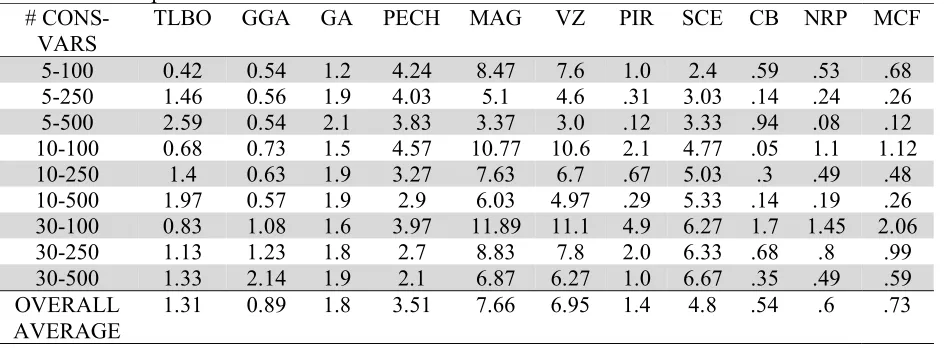
Recently, Rezoug et al. (2018) presented a guided genetic algorithm (GGA) to solve the MKP. In their paper, using the 270 MKPs from Beasley’s OR-Library, Rezoug et al. (2018) report in their Table 10 how their GGA performed compared to 9 solution approaches from the literature. These results along with our TLBO results are given in Table 2.
Table 2
Deviation from optimum #
CONS-VARS
TLBO GGA GA PECH MAG VZ PIR SCE CB NRP MCF
5-100 0.42 0.54 1.2 4.24 8.47 7.6 1.0 2.4 .59 .53 .68
5-250 1.46 0.56 1.9 4.03 5.1 4.6 .31 3.03 .14 .24 .26
5-500 2.59 0.54 2.1 3.83 3.37 3.0 .12 3.33 .94 .08 .12
10-100 0.68 0.73 1.5 4.57 10.77 10.6 2.1 4.77 .05 1.1 1.12
10-250 1.4 0.63 1.9 3.27 7.63 6.7 .67 5.03 .3 .49 .48
10-500 1.97 0.57 1.9 2.9 6.03 4.97 .29 5.33 .14 .19 .26
30-100 0.83 1.08 1.6 3.97 11.89 11.1 4.9 6.27 1.7 1.45 2.06
30-250 1.13 1.23 1.8 2.7 8.83 7.8 2.0 6.33 .68 .8 .99
30-500 1.33 2.14 1.9 2.1 6.87 6.27 1.0 6.67 .35 .49 .59
OVERALL
AVERAGE 1.31 0.89 1.8 3.51 7.66 6.95 1.4 4.8 .54 .6 .73
80
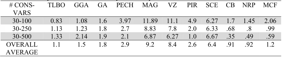
operator, New Reduction (Pirkul) NRP operates a lagrangian dual relaxation on MKP, and the Modified Choice Function-Late Acceptance Strategy (MCF). The reader should consult Rezoug et al. (2018) for more details. When a paper develops several metaheuristics and empirically evaluates them based on test problem instances available (typically on the WWW) to researchers, usually some statistical analysis is appropriate to determine which results are statistically better than other results. However, metaheuristics are not necessarily compared in a statistical manner to previously published metaheuristics. In this paper, we only developed one metaheuristic. To compare our results with other published metaheuristic results would be very difficult. Either we would have to code these procedures or we would have to request other researchers to share their results or code with us. Both of these seemed restrictive since the purpose of this paper is just to show that our simple TLBO approach for the MKP is reasonably “competitive” with other published MKP solution approaches. In other words, we were not interested in trying to (statistically) prove that our TLBO approach was better than any of the 10 approaches reported in Table 10 of Rezoug et al. (2018), we just wanted to show that it was competitive, while requiring considerably less effort to code, test and implement. From Table 2, we see that our TLBO is competitive with the other 10 solution approaches. We also see from Table 2, that TLBO performs better on the problems with 30 constraints. In Table 3, we focus on the 30 constraint problem instances (usually an MKP is considered to be more difficult as the number of constraints increase).
Table 3
Deviation from optimum for 30 constraint problem only #
CONS-VARS
TLBO GGA GA PECH MAG VZ PIR SCE CB NRP MCF
30-100 0.83 1.08 1.6 3.97 11.89 11.1 4.9 6.27 1.7 1.45 2.06
30-250 1.13 1.23 1.8 2.7 8.83 7.8 2.0 6.33 .68 .8 .99
30-500 1.33 2.14 1.9 2.1 6.87 6.27 1.0 6.67 .35 .49 .59
OVERALL
AVERAGE 1.1 1.5 1.8 2.9 9.2 8.4 2.6 6.4 .91 .92 1.2
In Table 3, we see that for the larger (usually more difficult) problems, TLBO is actually very competitive. In this case, only two solution procedures have smaller deviations from optimum (and not by much) than TLBO. Furthermore, these two solution procedures that gave slightly better solutions than TLBO for the 90 problem instances with 30 constraints each were definitely more complicated than TLBO. Specifically, the one procedure (CB) used a GA augmented with a feasibility and constraint operator which utilizes problem-specific knowledge and repair operators which locally improve the offspring. The other solution procedure (NR(P)) that was slightly better than TLBO used a lagrangian dual relaxation combined with a non-trivial dynamic estimation of the core size. TLBO is clearly simpler to code and implement than these two procedures with negligible sacrifice in solution quality.
5. Summary and Implications for Operations Research Practitioners
A major benefit of our results is that they can easily be used by operations research practitioners to solve industrial problems that cannot be solved efficiently with exact solution procedures. Furthermore, in a real-world situation when the optimal solution is not known, the practitioner can very easily build his/her confidence in the answer obtained from our procedure by simply putting it in a loop and executing it several times (do NOT reset the random number seed) and choosing the best answer obtained.
References
Akçay, Y., Li, H., & Xu, S. H. (2007). Greedy algorithm for the general multidimensional knapsack problem. Annals of Operations Research, 150(1), 17.
Baroni, M. D. V., & Varejão, F. M. (2015, November). A shuffled complex evolution algorithm for the multidimensional knapsack problem. In Iberoamerican Congress on Pattern Recognition (pp. 768-775). Springer, Cham.
Boyer, V., Elkihel, M., & El Baz, D. (2009). Heuristics for the 0–1 multidimensional knapsack problem. European Journal of Operational Research, 199(3), 658-664.
Chu, P. C., & Beasley, J. E. (1998). A genetic algorithm for the multidimensional knapsack problem. Journal of Heuristics, 4(1), 63-86.
Fréville, A. (2004). The multidimensional 0–1 knapsack problem: An overview. European Journal of
Operational Research, 155(1), 1-21.
Frieze, A. M., & Clarke, M. R. B. (1984). Approximation algorithms for the m-dimensional 0-1 knapsack problem: worst-case and probabilistic analyses. European Journal of Operational Research, 15(1), 100-109.
Baghel, M., Agrawal, S., & Silakari, S. (2012). Survey of metaheuristic algorithms for combinatorial optimization. International Journal of Computer Applications, 58(19), 2709-2716.
Kellerer, H., Pferschy, U., & Pisinger, D. (2004). Multidimensional Knapsack Problems. In Knapsack
problems(pp. 235-283). Springer, Berlin, Heidelberg.
Kong, X., Gao, L., Ouyang, H., & Li, S. (2015). Solving large-scale multidimensional knapsack problems with a new binary harmony search algorithm. Computers & Operations Research, 63, 7-22.
Laabadi, S., Naimi, M., El Amri, H., & Achchab, B. (2018). The 0/1 Multidimensional Knapsack Problem and Its Variants: A Survey of Practical Models and Heuristic Approaches. American Journal
of Operations Research, 8(05), 395.
Labed, S., Gherboudj, A.,& Chikhi, S. (2011) A Modified Hybrid Particle Swarm Optimization Algorithm for Multidimensional Knapsack Problem, International Journal of Computer Applications,
34(2), 11-16.
Lanza-Gutierrez, J. M., Crawford, B., Soto, R., Berrios, N., Gomez-Pulido, J. A., & Paredes, F. (2017). Analyzing the effects of binarization techniques when solving the set covering problem through swarm optimization. Expert Systems with Applications, 70, 67-82.
Meng, T., & Pan, Q. K. (2017). An improved fruit fly optimization algorithm for solving the multidimensional knapsack problem. Applied Soft Computing, 50, 79-93.
Moraga, R. J., DePuy, G. W., & Whitehouse, G. E. (2005). Meta-RaPS approach for the 0-1 multidimensional knapsack problem. Computers & Industrial Engineering, 48(1), 83-96.
Newhart, D. D., Stott, K. L., & Vasko, F. J. (1993). Consolidating product sizes to minimize inventory levels for a multi-stage production and distribution system. Journal of the operational Research
Society, 44(7), 637-644.
Rao, R. V., Savsani, V. J., & Vakharia, D. P. (2011). Teaching–learning-based optimization: a novel method for constrained mechanical design optimization problems. Computer-Aided Design, 43(3), 303-315.
Rezoug, A., & Boughaci, D. (2016). A self-adaptive harmony search combined with a stochastic local search for the 0-1 multidimensional knapsack problem. International Journal of Bio-Inspired
Computation, 8(4), 234-239.
82
Vasko, F. J., Wolf, F. E., & Stott, K. L. (1989). A practical solution to a fuzzy two-dimensional cutting stock problem. Fuzzy Sets and Systems, 29(3), 259-275.
Vasko, F. J., Wolf, F. E., & Pflugrad, J. A. (1991). An efficient heuristic for planning mother plate requirements at Bethlehem Steel. Interfaces, 21(2), 1-7.
Vasko, F. J., Wolf, F. E., Stott, K. L., & Woodyatt, L. R. (1993). Adapting branch-and-bound for real-world scheduling problems. Journal of the Operational Research Society, 44(5), 483-490.
Vasko, F. J., Newhart, D. D., & Strauss, A. D. (2005). Coal blending models for optimum cokemaking and blast furnace operation. Journal of the Operational Research Society, 56(3), 235-243.
Vasko, F. J., & Stott, K. L. (2008). Strategic Planning: OR to the Rescue. OR Insight, 21(3), 26-32.
Vasko, F.J., Lu, Y., & Zyma, K. (2016). An empirical study of population-based metaheuristics for the multiple-choice multidimensional knapsack problem, International Journal of Metaheuristics, 5(3-4), 193-225.
Vasko, F.J., & Y. Lu, Y.(2017). Binarization of continuous metaheuristics to solve the set covering problem: Simpler is better. invited talk, 21st Triennial Conference of The International Federation of Operational Research Societies (IFORS), Quebec, Canada, July 17-21, 2017.
Zyma, K., Lu, Y., & Vasko, F.J. (2015). Teacher training enhances the teaching-learning-based optimization metaheuristic when used to solve multiple-choice multidimensional knapsack problems,
International Journal of Metaheuristics, 4(3-4), 268-293.