www.atmos-meas-tech.net/7/2273/2014/ doi:10.5194/amt-7-2273-2014
© Author(s) 2014. CC Attribution 3.0 License.
Towards a consistent eddy-covariance processing:
an intercomparison of EddyPro and TK3
G. Fratini1and M. Mauder2
1LI-COR Biosciences Inc., Lincoln, Nebraska, USA
2Karlsruhe Institute of Technology, Institute of Meteorology and Climate Research – Atmospheric Environmental Research,
Garmisch-Partenkirchen, Germany
Correspondence to: G. Fratini ([email protected])
Received: 17 December 2013 – Published in Atmos. Meas. Tech. Discuss.: 4 March 2014 Revised: 28 May 2014 – Accepted: 24 June 2014 – Published: 29 July 2014
Abstract. A comparison of two popular eddy-covariance software packages is presented, namely, EddyPro and TK3. Two approximately 1-month long test data sets were processed, representing typical instrumental setups (i.e., CSAT3/LI-7500 above grassland and Solent R3/LI-6262 above a forest). The resulting fluxes and quality flags were compared. Achieving a satisfying agreement and understand-ing residual discrepancies required several iterations and in-terventions of different nature, spanning from simple soft-ware reconfiguration to actual code manipulations. In this pa-per, we document our comparison exercise and show that the two software packages can provide utterly satisfying agree-ment when properly configured. Our main aim, however, is to stress the complexity of performing a rigorous comparison of eddy-covariance software. We show that discriminating ac-tual discrepancies in the results from inconsistencies in the software configuration requires deep knowledge of both soft-ware packages and of the eddy-covariance method. In some instances, it may be even beyond the possibility of the inves-tigator who does not have access to and full knowledge of the source code. Being the developers of EddyPro and TK3, we could discuss the comparison at all levels of details and this proved necessary to achieve a full understanding. As a result, we suggest that researchers are more likely to get compara-ble results when using EddyPro (v5.1.1) and TK3 (v3.11) – at least with the setting presented in this paper – than they are when using any other pair of EC software which did not undergo a similar cross-validation.
As a further consequence, we also suggest that, to the aim of assuring consistency and comparability of central-ized flux databases, and for a confident use of eddy fluxes
in synthesis studies on the regional, continental and global scale, researchers only rely on software that have been ex-tensively validated in documented intercomparisons.
1 Introduction
The eddy-covariance (EC) processing sequence to calcu-late turbulent fluxes from raw, high-frequency data is com-plex, depending on the chosen instruments, their deployment, the site characteristics and the atmospheric turbulence pe-culiarities. The software realizing this processing is analo-gously complex to develop, maintain, document and support. Overviews of popular software packages including detailed lists of their features is available in Foken et al. (2012) and in Aubinet et al. (2012). Such public EC software packages – designed and intended for the general public – are repeatedly tested and inter-compared, improved on the basis of users’ feedbacks and updated to catch up with new findings and re-finements to the EC processing methods. The resulting ro-bustness, quality and reliability are difficult to achieve other-wise.
systems (e.g., analyzers for new gases). Of course, some in-house software may well not have these characteristics, but considerable effort is required to maintain a high-quality standard and many groups do not have the capacity or re-sources to do that.
For our purposes, it is convenient to introduce a nomen-clature for the operations performed in EC software. In this paper, a processing scheme is the ensemble of all operations performed by the software, from the ingestion of raw data to the calculation of corrected fluxes. A processing step is any major operations in the processing scheme, for example, the tilt correction or the elimination of spikes. For a given processing step, several methods can be available in the lit-erature, and different packages can thus implement a pro-cessing step with different methods. Often, a given software supports multiple methods for some of the processing steps, freely selectable by users. It is also to be noted that the same processing scheme can be implemented differently in differ-ent packages, because in some cases also the order in which the steps are performed matters. In addition, some software performs iterations of (some) processing steps.
The impact of the entire post-processing typically amounts to 5–20 % for energy fluxes and more than 50 % for CO2 fluxes if open-path analyzers are used (Mauder and Foken, 2006). It is therefore not surprising that fluxes obtained from the same raw data processed with different software pack-ages usually do not agree completely. For energy fluxes, Mauder et al. (2007) found an agreement within 10–15 % in an intercomparison of six different public EC packages from renowned international research institutions, while Mauder et al. (2008) found an agreement within 5–10 % of the re-sulting CO2 fluxes when comparing seven packages used in CARBOEUROPE-IP. The larger discrepancies in the first study occurred because participants had applied different processing schemes, reflecting different opinions on the best way to process those particular data sets. In contrast, all de-velopers of the second study had followed the same pre-scribed processing scheme, based on the recommendations of Lee et al. (2004).
A certain agreement was reached by the eddy-covariance community as to which processing steps are necessary under which conditions, thus any EC software can be expected to allow the appropriate processing schemes. However, as men-tioned earlier, large uncertainty remains as to which method shall be adopted for each step, and which is the correct order in the processing sequence. Furthermore, plenty of arbitrari-ness is left to the developers as to how to implement a given method, because typically published papers do not describe methods in sufficient technical detail. Finally, refinements of existing methods and new findings continuously arise, which impose updates to EC software, as documented for exam-ple by the recent works on effects of humidity in closed-path measurements (Ibrom et al., 2007b; Fratini et al., 2012; Nordbo and Katul, 2013), angle-of-attack effects (Nakai and Shimoyama, 2012; Kochendorfer et al., 2012; Mauder, 2013)
and flux biases due to errors in concentration measurements (Fratini et al., 2014).
Differences in post-processing routines present themselves to the researcher who attempts a software intercompari-son as either systematic or random differences in resulting fluxes, which are part of the overall measurement uncer-tainty and therefore need to be characterized. Richardson et al. (2012) distinguish systematic errors associated with dif-ferent data processing choices into those that arise from de-trending or other kinds of high-pass filtering and those due to the choice of the coordinate rotation method. Moreover, inevitable limitations of instrumentation (e.g., finite time re-sponse and averaging volume) require corrections during the post-processing, which may cause additional discrepancies. Instrument-related issues may include spikes, power failure, high-frequency losses and effects of air density fluctuations (Richardson et al., 2012).
Causes for discrepancies during intercomparisons can be conveniently grouped into four classes: (C1) inaccuracies in software configuration that lead to unintended differences in the processing schemes; (C2) differences in the methods available in each software, for any given processing step; (C3) differences in the actual implementation of a given method or differences in the order in which processing steps are implemented; and (C4) implementation errors (bugs).
Class C4 differs from C2 and C3 in that the latter classes are the result of conscious choices of the developer, while bugs (C4) are obviously unintended, and ideally get fixed as soon as they are found. The only class of causes attributable exclusively to the user is C1. However, while performing an intercomparison, it is crucial to be aware of causes of classes C2 and C3, which may require a deep knowledge of the soft-ware under consideration and (C3) of its source code.
Assuming no bugs (C4) in the software, in intercompar-isons such as the one described in Mauder et al. (2008), cause of class C1 can be minimized or completely avoided (especially, as we will see, if the comparison is carried out in several iterations). This expectation can be generalized to any intercomparisons carried out by micrometeorologists who are experts on the packages under consideration. In such cases, discrepancies are only due to causes of classes C2 and C3, which can only be eliminated – if deemed necessary – through a modification of either software being tested.
configuration was not appropriate to perform a meaningful intercomparison.
Triggered by these considerations, in this paper we present an intercomparison of the two EC public software packages EddyPro and TK3, with the threefold aim of (i) showing that they can give utterly satisfying agreement in calculated fluxes; (ii) identifying the sources of residual discrepancies; (iii) stressing the complexity of performing a fair and rigor-ous software comparison that highlights genuine discrepan-cies, which shall eventually be regarded as an ineliminable source of uncertainty. To achieve these aims, we will present the evolution of our comparison, identifying and categorizing the reasons for observed differences, showing how the match improves by elimination of such causes, and discussing resid-ual differences. Note that, while we will occasionally make comments on the suitability of certain implementations, an objective evaluation of alternative methods that we will iden-tify as sources of mismatches is beyond the scope of this work.
EddyPro (www.licor.com/eddypro) and TK3 (Mauder and Foken, 2011) are two of the most popular EC packages that are freely available, with about 3300 downloads in over 150 countries and more than 870 downloads in more than 53 countries to date.
EddyPro is a free of charge, open-source software re-leased by LI-COR Biosciences Inc. (Lincoln, NE, USA) un-der the GPL license. It was firstly released in April 2011 as EddyPro Express 2.0. Its code base builds entirely on ECO2S (the Eddy Covariance Community Software), an open-source software project started in 2007 at the University of Tuscia (Viterbo, Italy) and partially funded by the IMECC (http://imecc.ipsl.jussieu.fr/) and ICOS (www.icos-infrastructure.eu) European projects. Before re-lease, ECO2S was officially tested in a software intercompar-ison and results are documented in an IMECC project report. At the time of writing this paper, EddyPro version 5.1.1 in-cluded various options for each processing step required in the eddy-covariance chain.
The history of TK3 can be traced back over more than twenty years. It started with the Turbulenzknecht program which was first used to automatically compute turbulent fluxes in 1989. Its major assets were the elaborate quality as-sessment routines, which were unique at the time (Foken and Wichura, 1996). After more than ten years of successful ap-plication in many micrometeorological field campaigns the software was redeveloped from scratch in order to utilize the rapid advancements in computer technology and to allow for automatic processing of much longer data sets for up to one year. The resulting TK2 software included all state of the art flux corrections (Lee et al., 2004) and was extensively com-pared with other publically available EC-software (Mauder et al., 2008). Its updated version TK3 is in continuation of this lineage. TK3 is technically not open-source software; how-ever, selected parts of the code can be made available for inspection upon request.
We started our comparison using EddyPro v.5.0 and TK3 v3.11. As we will see, the intercomparison triggered some modifications to EddyPro which are already available in the current version 5.1.1, while the implementation of the despiking method of Mauder et al. (2013) in EddyPro is planned for a forthcoming release (see Sect. 3.1).
2 Comparison strategy
Two test data sets were selected with the intention to be representative of long-term flux observation setups (see Ta-ble 1). They both cover a period longer than 1 month in order to represent different weather conditions during the growing season. The closed-path data set originates from the Hainich EC station above a beech forest, which was part of the CARBOEUROPE-IP network (Knohl et al., 2003). This system consists of a Solent R3 sonic anemometer (Gill In-struments Ltd., UK) and a LI-6262 closed-path gas analyzer (LI-COR Biosciences) at a measurement height of 45 m. The open-path data set is from an EC system above a grass-land located near Graswang, Germany (Mauder et al., 2013), which is part of the Terrestrial Environmental Observatories network TERENO (Zacharias et al., 2011). The measure-ment height was 3.1 m and the instrumeasure-mentation consisted of a CSAT3 sonic anemometer (Campbell Scientific Inc., Logan, UT, USA) and a LI-7500 open-path gas analyzer (LI-COR Biosciences Inc.).
In our comparison, we considered results obtained for fric-tion velocity (u∗, m s−1), CO2 fluxes (Fc, µmol m−2s−1), latent heat fluxes (LE, W m−2), sensible heat fluxes (H, W m−2)and all corresponding quality flags according to the CARBOEUROPE-IP 0/1/2 scheme (Foken et al., 2004). We intentionally started the comparison with a generic definition of the processing scheme, of the kind that an average user would make. We stress again that, having full knowledge and control of the software code, we could in principle agree on the finest details at the onset, and have the software provide the exact same results at the first trial (provided the codes are free of bugs), but this would be of little help as it would not replicate any realistic situation. Instead, we strived to simu-late the typical starting point of an investigator who attempts an intercomparison, thus assuming proper knowledge of the EC method and of configuration of the two software pack-ages, but not sufficient control over the source code. In fact, having access to the source code of software packages com-prised of tens of thousands of code lines does not automat-ically grant the ability to understand it or meaningfully and safely modify it. We note here that this consideration applies to any EC software, both “public” and “in-house” as per the definitions provided in the introduction.
Table 1. Overview of the two test data sets: measured variables were wind componentsu,vandw, sonic temperatureTs, CO2and H2O concentration (either number densities or mole fractions) and air pressurep.
Data set closed-path open-path
Duration 49 days 38 days
Variables u, v, w, Ts, CO2, H2O u, v, w, Ts, CO2, H2O,p Instruments Solent R3/LI-6262 CSAT3/LI-7500
Ecosystem Forest Grassland
Measurement height 19 m 3.1 m
Tilt correction Planar fit Double rotation
class C2 and C3 (i.e., differences intrinsic to the software). In a couple of cases this exercise led to a revision/extension of either software, while some differences, assessed as being of class C2 (different methods for the same processing step), did remain and fully account for the residual differences.
After improving the match with the closed-path data set, we may have expected to need less than three rounds for the open-path one. However, open- and closed-path data exer-cise rather different parts of the code and for this reason we decided to do three rounds in both cases.
We decided to apply two different tilt corrections for the two data sets: double rotation for the open-path system and planar fit for the closed-path system (Wilczak et al., 2001) in order to test the agreement between the two packages with both methods. In accordance with the recommendations of Aubinet et al. (2012), we agreed on the processing scheme described in Table 2.
3 Results and discussion
The quality of the match between EddyPro and TK3 was quantified by deriving linear regressions (slope, intercept and r2) of the scatter plots of individual fluxes. Note that the choice of x andy axis for EddyPro and TK3 in the scatter plots was arbitrary and that – because of the independence of the two data sets – we opted for the symmetric RMA (reduced major axis) linear regression model. Furthermore, we considered the percentage of flux results for which the quality flags matched. Rather than presenting only the re-sult of the last round, in the following we shortly describe results obtained during the three rounds, to highlight the rea-sons for discrepancies and how we could improve the match in subsequent rounds. What we want to stress here is that some improvements were achieved by better tuning the con-figurations in order to perform the same operations in both EddyPro and TK3, while other improvements could only be achieved by intervening on the source code.
3.1 Closed-path data set
In the first round, results from the closed-path data set showed a general close agreement, however accompanied by
a significant number of scattering fluxes (Fig. 1). In addition, Fc showed a relatively large systematic bias (8 %) and the match of calculated quality flags was very poor: foru∗, LE andFc, only about 60 % of the obtained fluxes received the same quality flag from both packages. Only forH, the agree-ment was almost 90 % already.
Investigation revealed that one major difference of class C2 was hidden in the despiking processing step. In fact, TK3 implements the robust statistical method of Mauder et al. (2013) based on median absolute deviation (MAD), while the Gaussian statistical method of Vickers and Mahrt (1997) was used in EddyPro. This difference explained most of the observed scatter. Visual inspection and analysis of flux vari-ances showed that for those scattering points EddyPro re-sults were the implausible ones, giving variances>10 times larger than those of TK3, which instead fell into plausible ranges. Clearly, for those cases the despiking algorithm of Vickers and Mahrt (1997) – at least with the default settings used – was ineffective to remove large spikes in the raw data, which compromised the flux values. Since the newer despik-ing method of Mauder et al. (2013) proved to be more effec-tive in our case, the same algorithm was also implemented in EddyPro. Hence, the scatter was largely eliminated in the second round for all observed fluxes. Changes in the source code of EddyPro were required to make this possible, and the new implementation will be available to EddyPro users as an alternative despiking method in a forthcoming release. In the second round, the agreement between quality flags also slightly improved because of the improved comparability of the two packages after this modification. It is to be noted that the despiking method of Vickers and Mahrt (1997) is highly customizable. Therefore, we could have followed a different strategy and try and fine-tune that method in EddyPro until results matched satisfyingly. However, because of the sound-ness and simplicity of the MAD method, it was deemed ap-propriate to implement it in EddyPro and propose it as an option to its users.
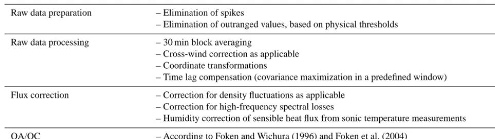
Table 2. Processing scheme for the software intercomparison
Raw data preparation – Elimination of spikes
– Elimination of outranged values, based on physical thresholds
Raw data processing – 30 min block averaging
– Cross-wind correction as applicable – Coordinate transformations
– Time lag compensation (covariance maximization in a predefined window)
Flux correction – Correction for density fluctuations as applicable – Correction for high-frequency spectral losses
– Humidity correction of sensible heat flux from sonic temperature measurements
QA/QC – According to Foken and Wichura (1996) and Foken et al. (2004)
as dry mole fractions (also called mixing ratios, moles of gas per mole of dry air) in TK3 and as mole fractions (moles of gas per mole of air) in EddyPro. Far from being a spe-cial occurrence in our comparison, it is often the case that concentration data are available without a clear indication of whether measurements are expressed as mole fractions or as dry mole fractions, as both units are normally reported as µmol mol−1 (or ppm) for CO
2 and as mmol mol−1 for H2O. The difference between the two is the dilution effect of H2O on CO2measurements (Webb et al., 1980; Ibrom et al., 2007a). Thus, in this case we confronted ourselves with a difference of class C1, a rather trivial but utterly common difference in the settings. Clearly agreeing on the nature of the measurements (which happened to be dry mole fractions) was sufficient to improve the slope of theFc regression by 6 %, from 0.92 to 0.97. Interestingly, we noted that this ad-justment had a negative effect on LE comparison, which ex-hibited a slope of 0.99 in the second round, and of 0.97 in the last one. Evidently, the seemingly perfect initial match was the result of systematic differences contributing in opposite directions and largely offsetting each other.
The differences observed in the calculated quality flags required deeper investigation, and highlighted several dif-ferences in the implementation: (i) the steady-state test was evaluated at different stages in the processing scheme; (ii) the quantities involved in the flag definition were slightly differ-ent; and (iii) the definition of the flag for the integral tur-bulence characteristics (ITC) was following different refer-ences: Foken et al. (2004) in TK3 and Göckede et al. (2004) in EddyPro. The agreement of the quality flags was greatly improved by reconsideration of these aspects in EddyPro. The group of TK3 developers has a long tradition in the def-inition of these quality flags, thus it was deemed appropri-ate to adapt EddyPro towards TK3, rather than the opposite. Nonetheless, residual discrepancies remained (up to 20 % for the quality flags of Fc)because difference (iii) was not ad-dressed. It is to be noted that, being both based on peer-reviewed published materials, there is no objective way to define a “better” implementation, so this difference (of class C2) shall be regarded as a source of ineliminable uncertainty.
Similarly, minor differences in the actual implementation of the quality flag assessment (for example, in EddyPro the sta-tionarity test is evaluated after coordinate rotation for tilt cor-rection, while in TK3 it is evaluated before that processing step: a difference of class C3) contribute to this uncertainty.
The remaining differences inFc and LE (about 3 %) are entirely explained by different spectral correction methods. TK3 implements the method of Moore (1986), based on ana-lytical transfer functions. Here, tube-dampening effects were taken into account by a first-order filter transfer function with 2 Hz cutoff frequency and the sensor separation in lateral direction was corrected according to Moore’s transfer func-tion while the longitudinal separafunc-tion had already been elim-inated by the time lag compensation. EddyPro supports sev-eral spectral correction schemes, including a few accounting for relative humidity (RH) dependent effects on water va-por fluxes (Ibrom et al., 2007b; Fratini et al., 2012). For the current comparison, the method described in Horst (1997) was selected because, among the ones not accounting for RH effects, it is the only one for which a cutoff frequency of 2 Hz could be prescribed a priori. Effects of lateral separa-tion were accounted for following the method of Horst and Lenschow (2009). For closed-path data, the spectral correc-tion is the last step in the chain (possibly before an iteracorrec-tion of the corrections, which was however not performed in our comparison) thus in this case it was easy to verify that the dif-ferent correction factors provided by difdif-ferent methods fully explained the residual difference inFcand LE which, again, shall be regarded as an intrinsic uncertainty.
3.2 Open-path data set
Figure 1. Scatter plots including RMA regression parameters foru∗,H, LE andFc, for the closed-path data set calculated with EddyPro and TK3. The results of the three comparison rounds with refined software configurations are displayed from left to right. Very poor regression parameters in the first round (leftmost plots) are driven by wildly scattering data points, lying outside the chart areas. The rightmost column shows the residuals of the linear regression for the third round.
During the first round, we observed a significant disper-sion, particularly forFc, and a systematic underestimation of Fcand LE in TK3 as compared to EddyPro (Fig. 2). The fol-lowing discussion highlighted that EddyPro was using baro-metric pressure (as estimated by site altitude) while TK3 was using pressure data available in the raw data files. That is, we incurred another discrepancy of class C1, and one worth dis-cussing. The pressure data in the raw files was not accompa-nied by metadata detailing its meaning, units and relevance to the eddy-covariance data. In this situation, the natural way of proceeding in EddyPro is to ignore this data and use baro-metric pressure instead. More in general, it is good practice to ignore data that are not fully documented. For example, in a closed-path system a pressure data may refer to, at least, the ambient air or the instrument’s cell: interpreting this data
in the wrong way would lead to significant systematic biases in fluxes. Seen from the opposite perspective, we suggest al-ways combining raw data with the metadata necessary to cor-rectly interpret it and use it during flux computation.
Once the software were set to use the pressure data from the raw files in the second round, most of the scatter was eliminated and we were left with systematic differences in Fcand LE of about 5–6 %. The agreement in quality flags is better than that at the first round of the closed-path compari-son with almost 70 % matching flags for all fluxes and even 92 % matching flags forH.
Figure 2. Same as Fig. 1, but for the open-path data set.
Moncrieff et al. (1997) was used in EddyPro. Different from the closed-path case, however, open-path data presents an ad-ditional complication when trying to entangle the effects of different spectral corrections from other potential sources of discrepancies. In fact, in this case the WPL terms – which are additive in nature – must be included after all fluxes have been corrected for spectral attenuations, and spectral corrections are thus no longer the last step in the processing scheme. To verify whether the difference in the spectral cor-rections solely accounted for the whole observed difference, in the third round we artificially (and only temporarily) mod-ified EddyPro to match on average (i.e., across the whole data set) the spectral correction factors calculated by TK3. After this operation, any residual systematic difference would have to be attached to the treatment of the WPL terms. Obviously, this manipulation is only possible if one has full control over (i.e., not only access to, but also appropriate knowledge of)
the software source code, while it would be relatively dif-ficult and error prone trying to do the same by proceeding backward from final fluxes.
as to how to implement it. The good matches achieved with both methods across the two data sets after the three rounds show that the implementations of TK3 and EddyPro are con-sistent, providing a sound cross-validation.
4 Conclusions
We have shown that, when properly configured, the two software packages EddyPro and TK3 provide satisfying, yet not perfect, agreement in calculated fluxes and related qual-ity flags. Initial comparisons highlighted discrepancies that could be eliminated by simply improving communication, exchanging more details on data significance and on the pro-cessing scheme. This suggests the importance of a very de-tailed consensus on EC post-processing to achieve the best possible comparability between fluxes processed by differ-ent users, even when using the same software, and of a very careful setup when an individual attempts the comparison be-tween two software packages.
Achieving further improvement required interventions on the source code, in particular with the implementation of the spike detection algorithm of Mauder et al. (2013) in Ed-dyPro, which is soon to become a standard option also in this software. The spectral correction procedures are quite different between EddyPro (Horst, 1997; Moncrieff et al., 1997) and TK3 (Moore, 1986). This is the processing step that caused the largest differences in flux results, differences that could not be eliminated using the current versions of the software. This finding suggests that further effort in the eddy-covariance methodology shall aim at reducing system-atic discrepancies obtained with different spectral correction approaches and methods.
Residual differences in quality flags were mostly due to different algorithms used for the well-developed turbulence test (Foken et al., 2004).
From our exercise, we conclude that discriminating among actual implementation errors, intentional differences and in-accuracies in the software configuration may only be possible to the investigator who has detailed knowledge of the source code and the ability to apply appropriate changes. The pre-sented comparison did not highlight any obvious bug (C4). All differences observed in the third round are explained in terms of different implementations of the same methods, or to the adoption of different methods. As a result of this effort and considering the results obtained in previous intercompar-isons (Mauder et al., 2007, 2008), we suggest that researchers are now more likely to get comparable results when using EddyPro (v5.1.1 and above) and TK3 (v3.11), than they are when using any other pair of EC software which did not un-dergo a similar cross-validation.
Generalizing our findings, we also conclude that an ex-haustive documentation of how fluxes are calculated from raw data should, whenever possible, include the details of the adopted processing scheme and possibly the name and
version of software used. Finally, we want to warn against ad hoc software intercomparisons as a means to validate (or invalidate) EC software, unless they are carried out by ex-perts of the software under considerations and with the re-quired level of detail, as demonstrated here. For the same rea-sons, when flux accuracy is of importance, we warn against the use of in-house software, if this does not undergo sys-tematic quality assurance procedures. In order to assure con-sistency and comparability of centralized flux databases, we rather suggest researchers to rely on public software pack-ages, notably those that are continuously QA/QC screened, and extensively validated in documented intercomparisons (e.g., Mauder et al., 2008, and this paper).
Acknowledgements. We wish to thank Mathias Herbst for
pro-viding the raw data set from the Hainich station. M. Mauder’s contribution was partly funded by the Helmholtz-Association through the President’s Initiative and Networking Fund. TERENO is funded by the Helmholtz Association and the German Federal Ministry of Education and Research.
Edited by: S. Malinowski
References
Aubinet, M., Vesala, T., and Papale, D. (Eds): Eddy Covariance: A Practical Guide to Measurement and Data Analysis, Springer, Berlin, 460 pp., 2012.
Foken, T. and Wichura, B.: Tools for quality assessment of surface-based flux measurements, Agr. Forest Meteorol., 78, 83–105, 1996.
Foken, T., Göckede, M., Mauder, M., Mahrt, L., Amiro, B. D., and Munger, J. W.: Post-field data quality control, in: Handbook of Micrometeorology. A Guide for Surface Flux Measurements, edited by: Lee, X., Massman, W. J., and Law, B. E., Kluwer, Dor-drecht, 181–208, 2004.
Foken, T., Leuning, R., Oncley, S. P., Mauder, M., and Aubinet, M.: Corrections and data quality, in: Eddy Covariance: A Practi-cal Guide to Measurement and Data Analysis, edited by: Aubi-net, M., Vesala, T., and Papale, D., Springer, Dordrecht, 85–132, 2012.
Fratini, G., Ibrom, A., Arriga, N., Burba, G., and Papale, D.: Rel-ative humidity effects on water vapour fluxes measured with closed-path eddy-covariance systems with short sampling lines, Agr. Forest Meteorol., 165, 53–63, 2012.
Fratini, G., McDermitt, D. K., and Papale, D.: Eddy-covariance flux errors due to biases in gas concentration measurements: origins, quantification and correction, Biogeosciences, 11, 1037–1051, doi:10.5194/bg-11-1037-2014, 2014.
Göckede, M., Rebmann, C., and Foken, T.: A combination of qual-ity assessment tools for eddy covariance measurements with footprint modelling for the characterisation of complex sites, Agr. Forest Meteorol., 127, 175–188, 2004.
Horst, T. W. and Lenschow, D. H.: Attenuation of scalar fluxes mea-sured with spatially-displaced sensors, Bound.-Lay. Meteorol., 130, 275–300, doi:10.1007/s10546-008-9348-0, 2009.
Ibrom, A., Dellwik, E., Larsen, S. E., and Pilegaard, K.: On the use of the Webb-Pearman-Leuning theory for closed-path eddy correlation measurements, Tellus B, 59, 937–946, 2007a. Ibrom, A., Dellwik, E., Flyvbjerg, H., Jensen, N. O., and Pilegaard,
K.: Strong low-pass filtering effects on water vapour flux mea-surements with closed-path eddy correlation systems, Agr. Forest Meteorol., 147, 140–156, 2007b.
Knohl, A., Schulze, E. D., Kolle, O., and Buchmann, N.: Large car-bon uptake by an unmanaged 250-year-old deciduous forest in Central Germany, Agr. Forest Meteorol., 118, 151–167, 2003. Kochendorfer, J., Meyers, T. P., Frank, J., Massman, W. J., and
Heuer, M. W.: How well can we measure the vertical wind speed? Implications for fluxes of energy and mass, Bound.-Lay. Meteo-rol., 145, 383–398, 2012.
Lee, X., Massman, W., and Law, B. E. (Eds): Handbook of Microm-eteorology, A Guide for Surface Flux Measurement and Analy-sis, Kluwer Academic Press, Dordrecht, 250 pp., 2004. Mauder, M.: A comment on “How well can we measure the
verti-cal wind speed? Implications for fluxes of energy and mass” by Kochendorfer et al., Bound.-Lay. Meteorol., 147, 329–335, 2013. Mauder, M. and Foken, T.: Impact of post-field data processing on eddy covariance flux estimates and energy balance closure, Me-teorol. Z, 15, 597–609, 2006.
Mauder, M. and Foken, T.: Documentation and Instruction Man-ual of the Eddy-Covariance Software Package TK3. Universität Bayreuth, Abteilung Mikrometeorologie 46, ISSN 1614-8924, 60 pp., 2011.
Mauder, M., Oncley, S. P., Vogt, R., Weidinger, T., Ribeiro, L., Bernhofer, C., Foken, T., Kohsiek, W., de Bruin, H. A. R., and Liu, H.: The Energy Balance Experiment EBEX-2000. Part II: Intercomparison of eddy-covariance sensors and post-field data processing methods, Bound.-Lay. Meteorol., 123, 29–54, 2007. Mauder, M., Foken, T., Clement, R., Elbers, J. A., Eugster,
W., Grünwald, T., Heusinkveld, B., and Kolle, O.: Quality control of CarboEurope flux data – Part 2: Inter-comparison of eddy-covariance software, Biogeosciences, 5, 451–462, doi:10.5194/bg-5-451-2008, 2008.
Mauder, M., Cuntz, M., Drüe, C., Graf, A., Rebmann, C., Schmid, H. P., Schmidt, M., and Steinbrecher, R.: A strategy for quality and uncertainty assessment of long-term eddy-covariance mea-surements, Agr. Forest Meteorol., 169, 122–135, 2013.
Moncrieff, J. B., Massheder, J. M., DeBruin, H., Elbers, J., Friborg, T., Heusinkveld, B., Kabat, P., Scott, S., Søgaard, H., and Ver-hoef, A.: A system to measure surface fluxes of momentum, sen-sible heat, water vapor and carbon dioxide, J. Hydrol., 188–189, 589–611, 1997.
Moore, C. J.: Frequency response corrections for eddy correlation systems, Bound.-Lay. Meteorol., 37, 17–35, 1986.
Nakai, T. and Shimoyama, K.: Ultrasonic anemometer angle of at-tack errors under turbulent conditions, Agr. Forest Meteorol., 162–163, 14–26, 2012.
Nordbo, A. and Katul, G.: A Wavelet-Based Correction Method for Eddy-Covariance High-Frequency Losses in Scalar Concentra-tion Measurements, Bound.-Lay. Meteorol., 146, 81–102, 2013. Richardson, A. D., Aubinet, M., Barr, A. G., Hollinger, D. Y., Ibrom, A., Lasslop, G., and Reichstein, M.: Uncertainty quan-tification, in: Eddy Covariance: A Practical Guide to Measure-ment and Data Analysis, edited by: Aubinet, M., Vesala, T., and Papale, D., Springer, Dordrecht, 173–210, 2012.
Vickers, D. and Mahrt, L.: Quality control and flux sampling prob-lems for tower and aircraft data, J. Atmos. Ocean. Technol., 14, 512–526, 1997.
Webb, E. K., Pearman, G. I., and Leuning, R.: Correction of the flux measurements for density effects due to heat and water vapour transfer, Q. J. Roy. Meteorol. Soc., 106, 85–100, 1980.
Wilczak, J. M., Oncley, S. P., and Stage, S. A.: Sonic anemometer tilt correction algorithms, Bound.-Lay. Meteorol., 99, 127–150, 2001.