Generalized Inverted Exponential Distribution
Amal S. Hassan
Department of Mathematical Statistics
Institute of Statistical Studies and Research (ISSR)/Cairo University, Egypt [email protected]
Marwa Abd-Allah
Department of Mathematical Statistics
Institute of Statistical Studies and Research (ISSR)/Cairo University, Egypt [email protected]
Heba F. Nagy
Department of Mathematical Statistics
Institute of Statistical Studies and Research (ISSR)/Cairo University, Egypt [email protected]
Abstract
This article deals with the estimation of R = P(Y < X) when X and Y are distributed as two independent generalized inverted exponential with common scale parameter and different shape parameters. The maximum likelihood and Bayesian estimators of R are obtained on the basis of upper record values and upper record ranked set samples. The Bayesian estimator cannot be obtained in explicit form, and therefore it has been achieved using Lindley approximation. Simulation study is performed to compare the reliability estimators in each record sampling scheme with respect to biases and mean square errors.
Keywords: Reliability; upper record ranked set sample; maximum likelihood estimator; Bayesian estimator; Lindley approximation.
1. Introduction
Abouammoh and Alshingiti (2009) introduced the generalized inverted exponential distribution ( ) as a generalization of the inverted exponential distribution. They declared that the can be better than the inverted exponential distribution for real data set based on the likelihood ratio test and the Kolmogorov-Smirnov statistic. The has been widely used in varied fields such as, accelerated life testing, horse racing, queues, sea currents and wind speeds.
The probability density function (pdf) of the with the shape parameter and the
scale parameter takes the following form
1 2
; , 1 x x ; 0, , 0.
f x e e x
x
(1)
The corresponding cumulative distribution function (cdf) is as follows
; ,
1 1 x ; 0, , 0.F x e x
Record data are very important in the situations that the observations are difficult to obtain or are destroyed in experimental tests. Record data arise in many real life applications such as industrial stress testing, meteorology, sports, hydrology and economics. A record value of some phenomenon is the largest (smallest) observation any one has ever made. The mathematical theory and statistical study of record values started by Chandler (1952) is now spread in many directions.The prominent theoretical contributions and inference issues may refer to Nagaraja (1988), Arnold et al. (1998) and Ahsanullah and Nevzorov (2015).
According to Arnold et al. (1998), record values can be classified into lower and upper record value (URV). For a sequence of independent and identically distributed (iid) random variables, an observation X j,j 1 is called an URV if its value exceed that all of previous observations
i e X. ., j Xi,for every i j
. While an observation is called alower record if its value is less than all previous observations
i e X. ., i X j, for every i j
.Suppose that the first m URV from cdf and pdf of the sampling population respectively, then the joint distribution of the first m
URV is defined by Arnold et al. (1998) as m 1
i 1
f ( , )
f ( , ) f( , ) ; ... ,
1 F( , ) i
m 1 m
i
u
u u u u
u
(3)
where u (u1,...,um), is the parameter space and may be a vector.
Ranked set sampling was first proposed by McIntyre in 1952 as a more efficient technique than simple random sample for estimating the population parameters of interest. Salehi and Ahmadi (2014) proposed a new sampling scheme for generating record data called record ranked set sampling to help scientists in situations where the only observations that are going to be used are the last record data such as athletic data, weather data and Olympic data. Since the new sampling scheme is based generally on ranked set sampling, so it is called record ranked set sampling.
As described by Salehi and Ahmadi (2014) for record ranked set sampling, suppose that there exist n independent sequential sequences of continuous random variables, the ith sequence sampling is terminated when the ith record value is observed. The only observations that are used for analysis are the last record value in each sequence. The last record value of the ith sequence in this plane is denoted by then the available observations are U (U1,1,U2,2,,Un n, )T , i.e.
where, ,
U
( )i j is the ith record in the jth sequence. It is recognized that unlike the record values; here Ui i, 'sare independent random variables but not ordered. Let, 1,1 2,2 ,
Ui i (U ,U ,,Un n)T be the upper record ranked set sample (URRSS), then the joint density function of
U
i i, , which is denoted by, ( , , ),
i i
U i i
f u is obtained using the marginal density of URV as follows
, ,1 ,
, 1
( )
( , ) ln 1 ; ( ; )
1 !
i i
i n
i i
i i i
U i i
u
f u F f u
i
(4)where,
u
i i,
u
1,1,
u
2,2,...,
u
n,n
Tis the observed values ofU
i i,,
is real valued parameter and is the parameter space.In reliability context, the parameter R = P(Y < X)is called stress-strength reliability. The stress-strength reliability arises naturally when we consider a random stress Y
applied to a certain device with strength X. If the stress exceeds the strength, i.e. Y >
X, the component will fail. Thus, the reliability is defined as the probability of not failing or P(Y < X). The reliability function R represents the relation between the stress and strength of the component, and it can be considered as a measure of a component performance.
The reliability function R = P(Y < X) has attracted the attention of many authors and become popular in many fields besides life testing, psychology, reliability and medical sciences. Lately, estimation of reliability function associated with record values have been raised in many fields such as industrial tests.
In recent years there has been a growing interest in the study of inference problems associated with stress-strength model and record values. The estimation problem of R =
P(Y < X) based on record values was firstly considered by Baklizi (2008) who estimated the reliability function based on URV for one and two parameters exponential distribution. Subsequent papers extended this work assuming various lifetime distributions for stress and strength random variables, for instance Baklizi (2012) estimated R based on URV for the Weibull distribution. Wang and Zhang (2013) estimated R for a class of distributions. Latterly, Salehi and Ahmadi (2015) considered the estimation of R based on URRSS from one-parameter exponential distribution and studied its performance.
This article aims to estimate the reliability function R = P(Y < X) when the strength and the stress are two independent variables of based on URV and URRSS. Assuming that the scale parameter is common and known, maximum likelihood and Bayesian estimators of R based on independent gamma priors for the unknown parameters are obtained under squared error loss function. The procedures of this study are encapsulated by analyzing a simulated data.
simulation study and numerical results are given in Section (4). Finally, conclusions appear in Section (5).
2. Maximum Likelihood Method of Estimation
This section provides the maximum likelihood (ML) estimator of R = P(Y < X) depending on the two record schemes, namely, URV and URRSS.
2.1 ML Estimator of R Based on URV
Let the random variable X represents the strength of the component available to overcome the stress Y applied on that component. Let X and Y be two independent
random variables from the with common scale parameter and different shape parameters
and respectively, then the reliability of a system is obtained as follows1 2
0
1 x x 1 1 x .
R e e e dx
x
(5)
To obtain the ML estimator of R; suppose u1,,um be URV observed from X
Let, also is URV observed from Y Therefore, the likelihood functions of , and for the observed samples u and s variables based on URV denoted by L( | ) u and L( | ) s are given by
1 2
1
( | ) 1 m i 1 i ,
m i i
u u u
L u e e
u e
(6)
and,
1 2
1
1 1
( | ) n j j .
n
s s
s
j j
L s e e e
s
(7)
The joint likelihood function of the observed record values u and s is given by
1 1
2 2
1 1
( , | , ) 1 m 1 n i 1 i j 1 j .
m n
s s
s
i i j j
u u u
L u s e e e e e
s
u e
The joint log-likelihood function of the observed record values u and s, denoted by l, is obtained as
1
1
ln ( , | , ) ln 1 ln 1 ln ln 2 ln ln 1
ln ln 2 ln ln 1 j .
m n i
m s
i
i i
n
s j
u u
j j
l L u s e e e
s e
s
u u
Assuming that the scale parameter is known, the ML estimators of
and , say ˆ and ˆ based on the observed URV can be obtained as the solutions ofln 1 um ,
l m e
and ln 1 n .
s l n e
(8)
From (8), we have
, ln 1 ˆ m u m e
and .
ln 1 ˆ n s n e (9)
Hence, by using the invariance property of ML estimation, then ML estimator of R, denoted by ˆR, becomes
1 ln 1 1 ln ˆ ˆ . ˆ ˆ 1 n m s u m e R n e (10)
2.2 ML Estimator of Based on URRSS
Let u1,1,,um m, and s1,1,,sn n, be two independent URRSS from the strength and stress random variables with parameters
,
and
,
respectively. Then the joint likelihood function of the observed URRSS ui i, and sj j, is obtained as follows, , , , , , 1 1
, , 2
1 ,
1
1 2
1 ,
[ ln(1 e )]
( , | , ) (1 e ) e
(i 1)!
[ ln(1 e )]
(1 e ) e .
(j 1)! i i
i i i i
j j
j j j j
u i m
u u
i i j j
i i i
s j n
s s
j j j
u s u s
The joint log-likelihood function of the observed URRSS ui i, and sj j, , denoted by l,is obtained as , , , , , 1 , , 1 ,
( 1) ln[ ln (1 )] ln{( 1)!} ln ln 2 ln (u ) ( 1) ln (1 )
( 1) ln[ ln (1 )] ln{( 1)!} ln ln 2 ln ( ) ( 1) ln (1 ) .
i i i i
j j j j
m
u u
i i
i i i
n
s s
j j
j j j
l i e i e
u
j e j s e
s
,
1
( 1)
ln 1 ,
2
i i
m
u i
l m m
e
and,
1
( 1)
ln 1 .
2
j j
n
s j
l n n
e
Assuming that the scale parameter is known, the ML estimators of
and , denoted by ˆˆ and ˆˆ are obtained as follows
,
1
1 ,
2 ln 1 ˆˆ i i u m i m m e
and
,
1
1
ˆˆ .
2 ln 1 j j
n s j n n e
(11)Hence, the ML estimator of R based on URRSS, denoted by R,ˆˆ is obtained by substituting
ˆˆ
and ˆˆ in (5) as follows
, , 1 1 1 1 ln 1ˆˆ 1 1 ˆˆ . ˆ ˆ n 1 ˆ l ˆ j j i i n u s j m i
m m e
R
n n e
(12)3. Bayesian Estimation
In this section, the Bayesian estimator of R is obtained under the assumption of independent gamma priors for the shape parameters
and . Bayes estimator of R is derived based on URV and URRSS using Lindley approximation.3.1 Bayesian Estimator of R Based on URV
According to Dey and Dey (2014), the gamma priors for the shape parameters and ,
and a squared error loss function (SELF) are used. Therefore, the prior densities of
and are
11 , a b e and, (13)
12 ,
c d
e
(14)
where a b c, , and d are the parameters of the prior distributions. Through combining the prior density (13) and the likelihood function (6), the posterior density of
can be obtained as follows
* 1
1 1 .
m
m a u b
e e
Similarly, through combining the prior density (14) and the likelihood function (7). The posterior density of is given by
* 1
2 1 .
n s
n c d
e e
(16)
Assume that
and
are independent, and let T1 1 eum
and 2 1 ,
n s
T e
the
joint bivariate posterior density of
and
will be
* 1 1
1 2
, | ,u s m a n c T eb T ed.
(17)By applying the transformation technique, let
B
r
and q
, (18)then
r q
B and
q
1rB
, q 0 , 0rB 1.Therefore, the joint bivariate posterior density function (17) can be written as
1 1 2 1
1 2
1 m a q rB r qB
* n m a c n c b d
B B B
r ,q | u, s q r r T e T e .
Consequently, the posterior pdf of
r
B can be formulated by integrating with respect to qas follows
[1 ]
1 1 2
1 2
* 0
1
[1 ]
1 1 2
1 2
0 0
(1 ) [ ] [ ]
( | , ) .
(1 ) [ ] [ ]
B B
B B
q r r q
n c m a n m a c b d
B B
B
q r r q
n c m a n m a c b d
B B B
r r q T e T e dq
r u s
r r q T e T e dq dr
(19)SELF implies the cost obtained by replacing the actual value of the parameter with the parameter estimate. Under SELF, the Bayes risk of R, is the expected value of
r
B.
This expected value contains an integral which is usually not obtained in a simple closed form
1
1
1 2
1 2
0 0 1
1
1 2
1 2
0 0
1
. 1
B B
B B
q r r q
m a
n c n m a c b d
B B B
B
q r r q
m a
n c n m a c b d
B B B
r r q T e T e dqdr
E r
r r q T e T e dqdr
,
R under SELF through Lindley's approximation form expanding about the posterior mode.
The Bayes estimator of R using SELF under URV cannot be computed analytically, therefore the Lindley's approximation is applied in the following subsection.
3.2 Lindley's Approximation of R Based on URV
It is known that the Bayes risk under SELF is the mean of the posterior distribution. Since the Bayes risk of R using SELF under URV cannot be computed analytically. Hence, the numerical calculations are needed by using Lindley's approximation for expanding the posterior mode. Consequently, Bayesian estimator of R say; R* is obtained. In the two parameters case ( , )
, Lindley's approximation leads to
30 12 21 12 12 21 03 21
1
ˆ [ ( , )] ( , )
2
B
U E U U B Q B Q C Q C Q B . (20)
where,
2 2 1 1
,
ij ij i j
B U
Q Q ; , 0,1, 2,3, 3,
for i,j1,2, and for i j, ii
ij j ii i
ij U U
B ( ) , Cij 3UiiiijUj(iijj2ij2),ij is the (i, j)th element in the inverse of the matrix Q* ( Q );*ij i, j 1, 2 such that
2 *
.
Q Q
In our case U( , ) R. The reliability function (5) is to be evaluated at ( ̃ ̃) which are the mode of the posterior density of URV. To show that the posterior density function is unimodal, it suffices to show that the function Q L( , ) ( , ) has the unique mode. Note that L
,
is a logarithm of the likelihood function and
,
is a logarithm of the joint prior distribution. Therefore, Q can be rewritten as
1 1 1
1 1 1
1 2
1 2
1 1 1
1 j 1 1
m n i
m m m
u s u
i
i i i i
n n n
s j
j j j j
Q ) ln( ) m ln ln u ) n ln
u
( m n ) ln ln s )
s
ln ( e e ln ( e
ln ( e a ln b c ln d .
.
The joint posterior mode, denoted by ( ̃ ̃) is obtained as ̃
and ̃
(21)
where, ln 1 eum
and ln 1 .
n
s
e
Therefore, the Bayes estimator of R based on URV can be obtained from (20) as follows
where, ̃ is the reliability function evaluated at ( ̃ ̃)
3.3 Bayesian Estimator of R Based on URRSS
The conjugate priors of both
and are assumed to be independent gamma distributions as defined in (14) and (15). Hence, the posterior density of
and is obtained, respectively, as follows
, 1 1 ** 1 1 , 1 m i i i mi a b u
i e e
and,
, 1 1 ** 2 1 . 1 n j j j nj c d s
j e e
Then, the joint bivariate posterior density of
and will be1 , ,
1
( ) 1 ( ) 1
** [ ]
, ,
1 1
( , | , ) ( ) ( ) (1 ) (1 ) .
n m
j i i j j
i
j c m n
i a
s u
b d i i j j
i j
u s e e e
By applying the transformation technique defined in Equation (18), therefore, the joint bivariate posterior density function can be written as
1 1
( ) 1 ( ) 1
**
, ,
( , | , ) (1 ) ( ) ,
n m j i j c i a
i i j j
B B B
r q u s r r D
where,
, , 1 1 1 2 1 1 11 1 .
m n j j i i B j B B B i q r q r m n
i j a c b r dr q s
i j
u
D q e e e
Consequently, the posterior pdf of rB is as follows
1 1 1 1 1 1 01 1 1
0 0 1 1 m n i j m n i j B B
i a j c
**
j , j
i a j c
B i ,i
B B B
r r Ddq
r , s .
r r Dd
u r | qd
Under SELF, the Bayes risk of R, is the expected value of rB. This expected value contains an integral which is usually not obtained in a simple closed form
1 1 1 1 1 1 0 01 1 1
0 0 1 , 1 m n i j m n i j
B B B
B
B B
i a j c
i a j c
B
r r Ddqdr
E r
r r Ddqdr
3.4 Lindley's Approximation of R Based on URRSS
Here, U( , ) R the reliability function (5) is evaluated at ( ̃̃ ̃̃) which is the mode of the posterior density; based on URRSS. In this case Q can be rewritten as
,
, ,
,
1 1 1
1 1 , 1 1
, 1
( 1)
ln ( 1) ln[ ln (1 ) ln{( 1)! 2 ln ( ) 2
1 ( 1)
( 1) ln (1 ) ln ( 1) ln[ ln (1 ) ln{( 1)! 2
(m n) ln 2 ln ( ) ( 1) ln (1 i i
j j i i
j
m m m
u
i i
i i i
m m n n
s
i i i i j j
n
s j j
j u
m m
Q i e i
n n
e j e j
u
s
u
e
,1 1 ,
1
) ( 1) ln
( 1) ln .
j
n n
j j j j
a b
s
c d
Again, the joint posterior mode based on URRSS, denoted by ( ̃̃ ̃̃) is obtained as
̃̃ 1 m i
i
W1and
̃̃ 1 n j
j
W2 ,
(22)
where, ,
1 1
W ln 1 i i
m i
u
e
and ,2 1
W ln 1 j j .
n
s j
e
The Bayesian estimator of R denoted by R**, based on URRSS can be obtained from (20) as follows
̃̃ * ( ̃̃ ̃̃ ̃̃ ( )
̃̃ ̃̃ ̃̃( )
̃̃ ̃̃ ̃̃( )
̃̃ ̃̃
̃̃( ))+,
where ̃̃ is the reliability function evaluated at ( ̃̃ ̃̃).
4. Simulation Study and Discussion
MSE
effˆ
,
ˆR
R ,
MS ˆˆ ˆ
R
E ˆR
and
** ** **
MSE R
eff R , R .
MSE R
The computations are performed based on 5000 replications using several combinations of the sample sizes (m,n) = (3,3), (3,6), (3,9), (5,5), (5,10), (6,3), (7,7), (9,3), (10,5),(10,10) and (12,12). Generate random samples from the GIED
,
and
GIED , using the transformation technique. The URV and URRSS are obtained for each of the strength and stress random samples. The ML estimate of R is computed based on URV and URRSS. Also, for a given values of the prior distributions parameters
4 2
a c , b d ,the Bayes estimates of R under SELF are obtained using Lindley approximation.
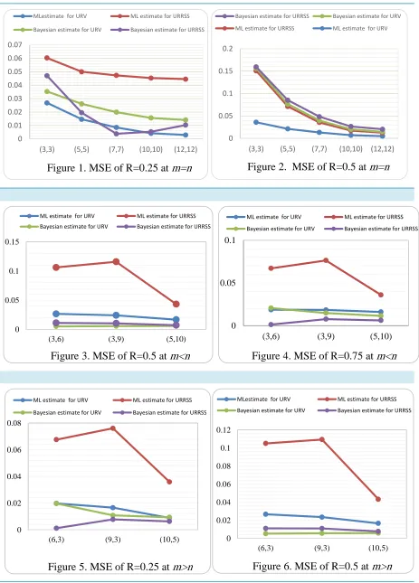
Tables 1 and 2 report the simulation results and represented for selected values of through Figures (1-6). From these tables and figures the following results can be observed
1. The ML estimate of R based on URV is more efficient than the corresponding based on URRSS for different sample sizes and different exact values of R (see Table 1). Also, the Bayesian estimator of R based on URRSS is more efficient than the corresponding based on URV for different sample sizes and different exact values of
R, expect few cases (see Table 2).
2. The MSE for the Bayesian estimates of R based on URV is less than the Bayesian estimate of R based on URRSS at R = 0. 5 for all m = n, m > n and m < n (see Figures 2, 3 and 6).
3. The MSE for the Bayesian estimate of R based on URRSS has the smallest values for
R = 0.75 when m < n (see Figure 4). Also, it has the smallest values for R = 0.25 when m > n (see Figure 5).
4. As seen from Figure 4, the MSEs for the ML estimate of R based on URV are less than the ML estimate of R based on URRSS at R = 0.75 for m < n.
Figures
0 0.01 0.02 0.03 0.04 0.05 0.06 0.07
(3,3) (5,5) (7,7) (10,10) (12,12)
Figure 1. MSE of R=0.25 at m=n
MLestimate for URV ML estimate for URRSS
Bayesian estimate for URV Bayesian estimate for URRSS
0 0.05 0.1 0.15 0.2
(3,3) (5,5) (7,7) (10,10) (12,12)
Figure 2. MSE of R=0.5 at m=n
Bayesian estimate for URRSS Bayesian estimate for URV
ML estimate for URRSS ML estimate for URV
0 0.05 0.1 0.15
(3,6) (3,9) (5,10)
Figure 3. MSE of R=0.5 at m<n
ML estimate for URV ML estimate for URRSS Bayesian estimate for URV Bayesian estimate for URRSS
0 0.05 0.1
(3,6) (3,9) (5,10)
Figure 4. MSE of R=0.75 at m<n
ML estimate for URV ML estimate for URRSS Bayesian estimate for URV Bayesian estimate for URRSS
0 0.02 0.04 0.06 0.08
(6,3) (9,3) (10,5)
ML estimate for URV ML estimate for URRSS Bayesian estimate for URV Bayesian estimate for URRSS
0 0.02 0.04 0.06 0.08 0.1 0.12
(6,3) (9,3) (10,5)
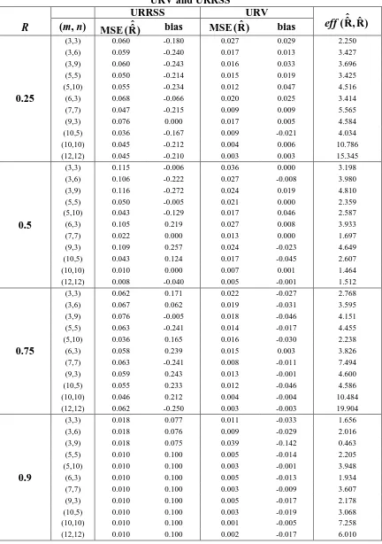
Table 1: MSE and bias for the ML estimates of R for different sample sizes based on URV and URRSS
R
URRSS URV ˆˆ ˆ
(R, R)
eff
(m, n) MSE(R) ˆˆ bias MSE ˆ(R) bias
0.25
(3,3) 0.060 -0.180 0.027 0.029 2.250
(3,6) 0.059 -0.240 0.017 0.013 3.427
(3,9) 0.060 -0.243 0.016 0.033 3.696
(5,5) 0.050 -0.214 0.015 0.019 3.425
(5,10) 0.055 -0.234 0.012 0.047 4.516
(6,3) 0.068 -0.066 0.020 0.025 3.414
(7,7) 0.047 -0.215 0.009 0.009 5.565
(9,3) 0.076 0.000 0.017 0.005 4.584
(10,5) 0.036 -0.167 0.009 -0.021 4.034
(10,10) 0.045 -0.212 0.004 0.006 10.786
(12,12) 0.045 -0.210 0.003 0.003 15.345
0.5
(3,3) 0.115 -0.006 0.036 0.000 3.198
(3,6) 0.106 -0.222 0.027 -0.008 3.980
(3,9) 0.116 -0.272 0.024 0.019 4.810
(5,5) 0.050 -0.005 0.021 0.000 2.359
(5,10) 0.043 -0.129 0.017 0.046 2.587
(6,3) 0.105 0.219 0.027 0.008 3.933
(7,7) 0.022 0.000 0.013 0.000 1.697
(9,3) 0.109 0.257 0.024 -0.023 4.649
(10,5) 0.043 0.124 0.017 -0.045 2.607
(10,10) 0.010 0.000 0.007 0.001 1.464
(12,12) 0.008 -0.040 0.005 -0.001 1.512
0.75
(3,3) 0.062 0.171 0.022 -0.027 2.768
(3,6) 0.067 0.062 0.019 -0.031 3.595
(3,9) 0.076 -0.005 0.018 -0.046 4.151
(5,5) 0.063 -0.241 0.014 -0.017 4.455
(5,10) 0.036 0.165 0.016 -0.030 2.238
(6,3) 0.058 0.239 0.015 0.003 3.826
(7,7) 0.063 -0.241 0.008 -0.011 7.494
(9,3) 0.059 0.243 0.013 -0.001 4.600
(10,5) 0.055 0.233 0.012 -0.046 4.586
(10,10) 0.046 0.212 0.004 -0.004 10.484
(12,12) 0.062 -0.250 0.003 -0.003 19.904
0.9
(3,3) 0.018 0.077 0.011 -0.033 1.656
(3,6) 0.018 0.076 0.009 -0.029 2.016
(3,9) 0.018 0.075 0.039 -0.142 0.463
(5,5) 0.010 0.100 0.005 -0.014 2.205
(5,10) 0.010 0.100 0.003 -0.001 3.948
(6,3) 0.010 0.100 0.005 -0.013 1.934
(7,7) 0.010 0.100 0.003 -0.009 3.607
(9,3) 0.010 0.100 0.005 -0.017 2.178
(10,5) 0.010 0.100 0.003 -0.019 3.068
(10,10) 0.010 0.100 0.001 -0.005 7.258
Table 2: MSE and bias for the Bayesian estimates of R for different sample sizes based on URV and URRSS
R
URRSS URV
eff (R*, R**) (m, n) MSE(R**) bias MSE (R*) bias
0.25
(3,3) 0.047 0.213 0.035 0.179 1.331
(3,6) 0.086 0.286 0.039 0.189 2.225
(3,9) 0.088 0.290 0.048 0.215 1.817
(5,5) 0.020 0.125 0.026 0.151 0.747
(5,10) 0.021 0.136 0.038 0.190 0.559
(6,3) 0.001 0.014 0.020 0.129 0.061
(7,7) 0.004 0.029 0.020 0.132 0.191
(9,3) 0.008 -0.085 0.011 0.090 0.722
(10,5) 0.006 -0.068 0.009 0.082 0.670
(10,10) 0.005 -0.062 0.016 0.118 0.340
(12,12) 0.010 -0.097 0.014 0.113 0.730
0.5
(3,3) 0.003 -0.001 0.005 0.000 0.644
(3,6) 0.011 0.072 0.005 0.012 2.161
(3,9) 0.010 0.074 0.006 0.037 1.837
(5,5) 0.009 -0.003 0.005 0.000 1.603
(5,10) 0.007 0.010 0.006 0.043 1.215
(6,3) 0.011 -0.072 0.005 -0.012 2.111
(7,7) 0.009 -0.001 0.004 0.000 2.074
(9,3) 0.011 -0.079 0.006 -0.039 1.947
(10,5) 0.008 -0.014 0.006 -0.043 1.322
(10,10) 0.007 0.000 0.003 0.001 2.418
(12,12) 0.006 -0.034 0.002 -0.001 2.799
0.75
(3,3) 0.048 -0.215 0.036 -0.184 1.325
(3,6) 0.001 0.015 0.021 -0.134 0.063
(3,9) 0.008 0.084 0.015 -0.111 0.519
(5,5) 0.063 -0.250 0.026 -0.149 2.441
(5,10) 0.006 0.067 0.012 0.012 0.539
(6,3) 0.087 -0.288 0.036 -0.182 2.414
(7,7) 0.063 -0.250 0.020 -0.133 3.103
(9,3) 0.088 -0.291 0.040 -0.194 2.201
(10,5) 0.022 -0.137 0.038 -0.189 0.576
(10,10) 0.005 0.063 0.016 -0.118 0.350
(12,12) 0.063 -0.250 0.014 -0.113 4.428
0.9
(3,3) 0.134 -0.364 0.094 -0.302 1.431
(3,6) 0.026 -0.158 0.057 -0.234 0.456
(3,9) 0.003 -0.051 0.057 -0.236 0.052
(5,5) 0.079 -0.274 0.067 -0.253 1.176
(5,10) 0.005 -0.062 0.032 -0.174 0.159
(6,3) 0.194 -0.436 0.095 -0.304 2.052
(7,7) 0.032 -0.170 0.051 -0.222 0.617
(9,3) 0.196 -0.438 0.103 -0.318 1.892
(10,5) 0.082 -0.282 0.078 -0.276 1.058
5. Conclusion
In this paper, the problem of estimating R = P(Y < X) for the is addressed using both URV and URRSS. ML and Bayesian estimators of R are compared via the MSE. Also, the efficiency of estimators based on URRSS with respect to the corresponding estimators based on URV is computed. When comparing the performance of the estimated R ,it is observed that the ML estimate based on the URV is, in general, better than the corresponding based on URRSS relative to their biases and MSEs. MSE of the Bayes estimate based on URRSS approach is less than the MSE of the corresponding ML estimate. The simulation study indicates that in order to estimate the reliability function in stress-strength model for using ML method of estimation, URV scheme is preferable than URRSS scheme.
Acknowledgement
The authors would like to thank the Editor-in-Chief and the anonymous referees for very helpful comments which greatly improved the paper.
References
1. Abouammoh, A. M. and Alshingiti, A. M. (2009). Reliability estimation of generalized inverted exponential distribution. Journal of Statistical Computation and Simulation, 79(11), 1301-1315.
2. Ahmad, K. E., Fakhry, M. E. and Jaheen, Z. F. (1997). Empirical Bayes estimation of P(Y<X) and characterizations of Burr-type X model. Journal of Statistical Planning and Inference, 64(2), 297-308.
3. Ahsanullah, M. and Nevzorov, V. B. (2015). Records via Probability Theory
(Vol. 6). Tampa, USA: Atlantis Press.
4. Arnold, B. C., Balakrishnan, N. and Nagaraja, H. N. (1998). Records. Wiley Series in Probability and Statistics. John Wiley & Sons, Inc.
5. Baklizi, A. (2008). Estimation of Pr(X<Y) using record values in the one and two parameter exponential distributions. Communications in Statistics-Theory and Methods, 37(5), 692-698.
6. Baklizi, A. (2012). Inference on P(Y<X) in the two-parameter Weibull model based on records. ISRN Probability and Statistics, 1-11.
7. Chandler, K. N. (1952). The distribution and frequency of record values. Journal of the Royal Statistical Society, 14(2), 220-228.
8. Dey, S. and Dey, T. (2014). Generalized inverted exponential distribution: different methods of estimation. American Journal of Mathematical and
9. Lindley, D. V. (1980). Approximate Bayesian methods. Trabajos de Estadistica,
31(1), 223-245.
10. Nadar, M. and Papadopoulos, A. S. (2011). Bayesian analysis for the Burr Type XII distribution based on record values. Statistica, 71(4), 421-435.
11. Nagaraja, H. N. (1988). Record values and related statistics- a review.
Communications in Statistics-Theory and Methods, 17(7), 2223-2238.
12. Raqab, M. Z. and Kundu, D. (2005). Comparison of different estimators of P(Y < X) for a scaled Burr type X distribution. Communications in
Statistics-Simulation and Computation, 34(2), 465-483.
13. Salehi, M. and Ahmadi, J. (2014). Record ranked set sampling scheme. Metron,
72(3), 351-365.
14. Salehi, M. and Ahmadi, J. (2015). Estimation of stress-strength reliability using record ranked set sampling scheme from the exponential distribution. Filomat,
29(5), 1149-1162.