www.solid-earth.net/5/1087/2014/ doi:10.5194/se-5-1087-2014
© Author(s) 2014. CC Attribution 3.0 License.
Using the level set method in geodynamical modeling of
multi-material flows and Earth’s free surface
B. Hillebrand1, C. Thieulot1,2, T. Geenen3, A. P. van den Berg1, and W. Spakman1,2 1Department of Earth Sciences, Utrecht University, the Netherlands
2Centre of Earth Evolution and Dynamics (CEED), University of Oslo, 0316 Oslo, Norway 3SurfSara, Amsterdam, the Netherlands
Correspondence to: B. Hillebrand ([email protected])
Received: 4 June 2014 – Published in Solid Earth Discuss.: 9 July 2014
Revised: 25 September 2014 – Accepted: 8 October 2014 – Published: 18 November 2014
Abstract. The level set method allows for tracking material surfaces in 2-D and 3-D flow modeling and is well suited for applications of multi-material flow modeling. The level set method utilizes smooth level set functions to define ma-terial interfaces, which makes the method stable and free of oscillations that are typically observed in case step-like tions parameterize interfaces. By design the level set func-tion is a signed distance funcfunc-tion and gives for each point in the domain the exact distance to the interface as well as on which side it is located. In this paper we present four bench-marks which show the validity, accuracy and simplicity of using the level set method for multi-material flow model-ing. The benchmarks are simplified setups of dynamical geo-physical processes such as the Rayleigh–Taylor instability, post-glacial rebound, subduction and slab detachment. We also demonstrate the benefit of using the level set method for modeling a free surface with the sticky air approach. Our results show that the level set method allows for accurate ma-terial flow modeling and that the combination with the sticky air approach works well in mimicking Earth’s free surface. Since the level set method tracks material interfaces instead of materials themselves, it has the advantage that the location of these interfaces is accurately known and that it represents a viable alternative to the more commonly used tracer method.
1 Introduction
Accurate modeling of geodynamical processes involving large deformation, e.g., mantle flow, subduction evolution or slab tearing, is a key research goal in computational
geody-namics. Since the early simplified two-dimensional isother-mal model configurations (Gurnis and Hager, 1988; Chris-tensen, 1996), model complexity and especially the num-ber of materials present in numerical models has dramati-cally increased as seen in recent three-dimensional thermo-mechanically coupled models that include multiple materials and phase changes as well as surface deformation and com-plex rheologies (e.g., van Hunen and Allen, 2011; Duretz et al., 2014). For instance multiple materials are important to investigate the influence of an oceanic crust on the decou-pling of subducting and overriding plates as well as on the buoyancy of the subducting slab (Bˇehounková and ˇCižková, 2008; van Hunen and van den Berg, 2008; Androviˇcová et al., 2013); they are also important for research involving sub-duction termination by continental collision (e.g., Baumann et al., 2010; Magni et al., 2012). Other studies focus on the influence of complex rheologies on slab dynamics (Billen and Hirth, 2007; Andrews and Billen, 2009); finally, the aim of many recent studies has been to investigate the influence and response of a free surface in subduction modeling (e.g., Schmeling et al., 2008; Gerya et al., 2009; Quinquis et al., 2011; Duretz et al., 2011).
mesh may become too distorted and remeshing is required. This is computationally expensive, results in unwanted nu-merical diffusion and constitutes an important drawback for models with large deformation.
In Eulerian codes the mesh is fixed. Because of this ele-ments do not track materials and a method for material track-ing is needed. The two more commonly used methods in computational geodynamics are the marker-in-cell technique and the phase field method.
Tracers (particles, markers) are widely used in the geo-dynamical community (e.g., Tackley and King, 2003; van Hunen and Allen, 2011; Duretz et al., 2012). These La-grangian particles are advected with the flow and carry ma-terial properties such as density and viscosity. Velocity equa-tions are solved on the finite element mesh and the veloci-ties used to advect the particles are obtained from interpo-lation. One element generally contains several up to 100s of particles. This method easily allows for advection of multi-material fields using an Eulerian mesh and is potentially non-diffusive (Tackley and King, 2003). While the tracer method tracks materials and has as an advantage that it can record its history, it does however not track the interface between the materials. The interface position remains approximate and is known with an uncertainty on the order of local tracer dis-tance. However, the tracer method tracks materials, it does not track the interface between the materials. The interface position remains approximate and is known with an uncer-tainty on the order of local tracer distance. Furthermore, the tracer method becomes increasingly expensive in 3-D. For instance, in the 2-D models of Crameri et al. (2012) the dif-ferent codes used between ten and hundreds of particles per element/cell. In 3-D this translates to several dozens up to thousands of particles per element/cell, i.e., possibly billions in total in the case of large 3-D simulations. The computa-tional as well as the memory costs would then become huge, requiring that the code is highly parallel and scales up to hun-dreds of cores or more.
In the phase field method (Lenardic and Kaula, 1993; Van Keken et al., 1997; Kronbichler et al., 2012), materi-als are assigned a number, and the composition of the fluid at a given node of the grid is given by a field containing the various fractions of the different material components. This field is then advected using a stabilized advection equation. The phase field vector is only defined on the nodal points of the mesh; thus, the computational costs increase proportion-ally to the increase in nodal points. However, such a phase field will contain sharp contrasts between the different phases within elements and the advection of the phase field requires complex stabilization schemes (Lenardic and Kaula, 1993).
In this paper we explore a third method, the level set method that, instead of tracking materials, is geared to track the material interfaces. The method is based on defining a level set function (generally signed distance) which is zero at the target interface and positive on one side and negative on the other side. This signed property is used to identify the
dif-ferent materials. Similar to the phase field method the level set function is defined on the nodal points of the elements and the computational costs increase proportional to the increase in nodal points. In contrast with the phase field method, the level set method does not involve step-like discontinuities but instead represents fields with a smooth (signed distance) function (the level set function). The level set method pro-vides a sharp location for the interface.
The level set method has not often been used in the geo-dynamical community. Notable exceptions are Hale et al. (2007), Gross et al. (2007) and Bourgouin et al. (2007) which are focussed on lava dome growth and/or mantle plumes, Suckale et al. (2010) on bubbles dynamics in volcanic con-duits, Zlotnik et al. (2008) on gravitational instabilities and Hale et al. (2010) on slab tear faults. In Braun et al. (2008) a level set method is presented which is based on a 3-D set of triangulated points, which makes it a hybrid between trac-ers and level set functions. The level set method is primarily used in other fields of computational science such as two-phase flows (Oka and Ishii, 1999) and fluid dynamics (Rao et al., 2011). An overview of the method and applications can be found in Osher and Fedkiw (2001).
In this paper we present four benchmarks of increasing complexity and end with applications to modeling of subduc-tion and slab detachment. Two of the presented benchmarks include deformation of Earth’s free surface. In Eulerian-based codes this is generally modeled either by ALE (arbi-trary Lagrangian–Eulerian; Fullsack, 1995; Thieulot, 2011) methods or the so-called sticky air approach (Schmeling et al., 2008; Crameri et al., 2012). In ALE the top layers of elements can deform vertically. The sticky air approach en-tails that an air layer of low viscosity and zero density is put atop the surface. This causes the Earth’s surface to become a boundary between two materials inside the model domain which we track using the level set method.
The purpose of our paper is to demonstrate the use of the level set method in various geodynamic applications and to demonstrate the applicability of the presented approach to more complex geodynamical processes.
2 Methods
All experiments in this paper are mechanical models inter-nally driven by density perturbations. They do not include any temperature effects. We use the finite element modeling package SEPRAN (Segal and Praagman, 2005) and solve for mass conservation of an incompressible fluid:
∇ ·v=0, (1)
and the Stokes equation describing a force balance:
−∇P+ ∇ ·σd=f(ρ). (2)
function of the material that is advected through the domain which is tracked by means of the level set method. The equa-tions are solved on linear triangular elements. The model-ing package SEPRAN has been used in geodynamical mod-eling for many years(e.g., ˇCížková et al., 2007; van Hunen and van den Berg, 2008; Chertova et al., 2012; Androviˇcová et al., 2013).
2.1 Level set method 2.1.1 Introduction
The level set method is a well-researched interface track-ing technique which was originally devised by Osher and Sethian (1988). It tracks an interface by defining it as the zero valued isocontour of a smooth function. In the last two decades several improvements and variations have been pre-sented by several authors such as reinitialization (see below) extension velocities (e.g., Adalsteinsson and Sethian, 1999; Chopp, 2009), local level set methods (e.g., Sethian, 2001), hybrid particle level set methods (e.g., Enright et al., 2002; Samuel and Evonuk, 2010), variational level set method (e.g., Duan et al., 2008) and the level set method combined with volume of fluid method (e.g., Fedkiw et al., 1999; Pijl et al., 2008).
The level set method implementation presented here is global and uses reinitialization to keep the level set function smooth. If0denotes the interface that is to be associated and tracked with a level set function φ, andis a bounded re-gion, bounded by just the interface or the interface and the boundaries of the model domain,φwill be defined as (Osher and Fedkiw, 2001):
φ (r, t ) >0 forr∈
φ (r, t ) <0 forr6∈ (3)
φ (r, t )=0 forr∈∂=0(t ).
The level set function is advected by means of the advection equation:
∂φ
∂t +v· ∇φ=0. (4)
This equation is solved using a Crank–Nicolson inte-gration scheme in combination with the streamline up-wind Petrov–Galerkin (SUPG) upup-wind scheme (Brooks and Hughes, 1982). The level set function is generally chosen to be a signed distance function which means that|∇φ| =1 ev-erywhere. The function value indicates on which side of the interface a point is located (negative or positive) and this is used to identify materials. Because the level set function is a signed distance function, its value is also the distance to the interface.
2.1.2 Reinitialization
The level set function is advected with a velocity field result-ing from the buoyancy forces. This velocity field does not
necessarily preserve the signed distance quality of the level set function. However, it has been shown by several authors (Sussman et al., 1995; Min, 2010) that it is important for the level set function to stay smooth in the vicinity of the zero level set (at least Lipschitz continuous; Osher and Fedkiw, 2001). Therefore, the level set function is corrected so that it remains a smooth function without moving the zero isocon-tour and thus the interface itself. Sussman et al. (1995) in-troduced a method called reinitialization which exploits the signed distance quality of the level set function. The reini-tialization process involves solving the following equation: ∂φ
∂τ =sign(φ)(1− |∇φ|). (5)
This equation specifies a correction for the value of φ if
|∇φ| 6=1. ∂τ is a pseudo time step and sign(φ) is the one dimensional signum (or sign) function, and 0 atφ=0, for which generally a smooth approximation is used. Equa-tion (5) does not need to be solved every time step. We use an error criterion to determine whether reinitialization is needed and then solve several reinitialization iterations until our cri-terion is satisfied. The error is calculated by taking the aver-age of the deviation of the absolute gradient ofφ from one of all the nodal points. The number of iterations needed de-pends on the choice of∂τ, sign(φ) and the choice of the error criterion. For the smoothened sign function we use
sign(φ)= φ
p
φ2+(C1x)2. (6)
The value of constantC is arbitrarily chosen. A high value results in a slower (more iterations) but more stable reinitial-ization process while a low value has the opposite effect. In our modelsC=15 proved to be a practical compromise be-tween speed and stability. The determination of∇φis impor-tant for the reinitialization procedure and it needs to be robust for both small and large-scale variations. We therefore use a second order ENO (essentially non-oscillatory) scheme for the space derivative (Osher and Shu, 1991; Jiang and Peng, 2000). We also use a third order TVD (total variation dimin-ishing) Runge–Kutta scheme for the pseudo time integration of Eq. (5) (Gottlieb and Shu, 1998).
2.1.3 Usage of the level set method
We use the level set method to track the interface between two different (geological) materials, but we note that the ap-plication can involve any chosen surface. Every interface is described by its own level set function. Since the level set function is defined such that its zero isocontour coincides with the interface between two materials, one material will be where the function is negative and the other where it is positive. For an arbitrary material parameterC this can be written as
C= (
C1 forφ≤0 C2 forφ >0.
We coin this the sharp boundary method which results in sharp contrasts of material parameters (density, viscosity, etc.) within an element. One can also introduce a small dif-fusion zone around the interface (Bourgouin et al., 2006), hereafter called the diffuse boundary method. It is important to note that this does not mean that the location of the inter-face is no longer known. The location is still exactly known.
C=
C1 forφ≤ −αh
C2 forφ≥αh
(C2−C1)φ
2αh + (C1+C2)
2 for|φ|< αh
(8)
Hereα=1 andhrepresents one element size. When Eq. (8) is used to smooth density across the interface,Cis simply the density value; however, when viscosity is smoothened across the interface,Cis the exponent of viscosity (i.e., smoothing the logarithm of viscosity). The level set function is evalu-ated at the nodal points of the elements. Density and vis-cosity are thus assigned to the nodal points and then interpo-lated to the Gaussian integration points of the finite elements. A comparison between the two methods is performed with the Rayleigh–Taylor instability benchmark found in Sect. 4. In the other benchmarks the diffuse boundary method is used. Because of the signed distance quality of the level set func-tion, the zone of the diffuse boundary (2h) follows directly from the level set function values and no additional steps to identify this zone are required. The width (h) of the diffuse boundary is easily changed in case more smoothness is re-quired.
2.2 Sticky air approach
Several of the benchmark experiments we conduct will in-clude an approximation of the Earth’s free surface using the so-called sticky-air approach (Schmeling et al., 2008; Crameri et al., 2012). This allows modeling of topography changes while using a purely Eulerian code by augmenting the model with a top layer with so-called sticky-air. Since Earth’s surface is effectively a stress-free surface this layer of air should exert as little stress on the underlying lithosphere material as possible. Crameri et al. (2012) investigated the viscosity contrast and thickness of the sticky air layer and concluded that for a 100 km thick layer the viscosity of the air layer should be 5 orders of magnitude less than the un-derlying material. The density of the sticky air layer is set to zero so that it has no pressure effect on the real free surface (the sticky air–lithosphere interface).
3 Benchmarks
Here we present the model setups of the various benchmarks presented in this paper. All four benchmarks describe multi-material flow models and some include the modeling of
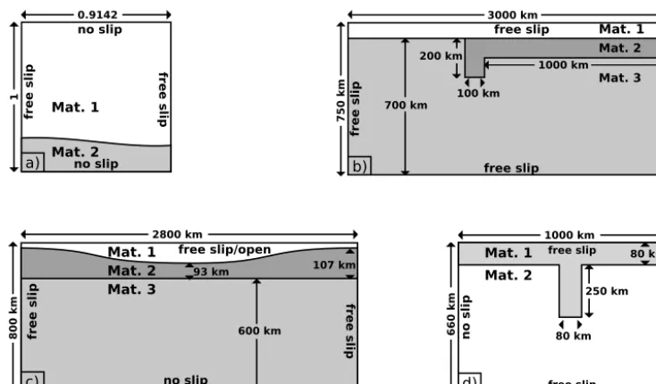
Earth’s free surface by means of a sticky air layer. The bench-marks are the Rayleigh–Taylor instability from Van Keken et al. (1997), the post-glacial rebound setup from Crameri et al. (2012), the free subduction benchmark from Schmeling et al. (2008) and the simplified slab detachment setup from Schmalholz (2011). The first benchmark models the overturn of a gravitationally unstable compositional layering and is of-ten used in the geodynamical modeling community. The sec-ond and third benchmark focus on the sticky air approach. The last benchmark setup demonstrates the splitting of one material domain into two. The setups of the benchmarks are illustrated in Fig. 1 and a small description of each follows below.
3.1 Rayleigh–Taylor instability
This benchmark represents a buoyancy driven flow and (Fig. 1a) has been performed by several authors with various techniques including tracers (Van Keken et al., 1997; Tackley and King, 2003), level set method (Bourgouin et al., 2006), particle level set method (Samuel and Evonuk, 2010), phase field method (Bangerth and Heister, 2013) and a marker chain method (Van Keken et al., 1997). The benchmark de-scribes an almost square domain of unit height and a width of 0.9142, in which a dense layer overlies a lighter layer. The interface geometry between the two layers is given by a sine function defined asw(x)=0.02 cos(π xλ )+0.2 with λ=0.9142. We will compare snapshots at regular intervals with the snapshots of the original article (Van Keken et al., 1997). We will also compare the evolution of the root mean square velocity(vrms) of the entire domain over time, specifi-cally concentrating on the timing and height of the first peak, which coincides with the rise of the first diapir. Thevrmsis given by
vrms=
s
1 V
Z
||v||2dv. (9)
HereV is the volume of the domain. 3.2 Post-glacial rebound
80
0
k
m
2800 km
600 km
fr
ee
s
li
p
fr
ee
sl
ip
no slip
free slip/open
Mat. 1 Mat. 2 Mat. 3
107 km 93 km
1
0.9142
no slip
no slip
fr
ee
sl
ip free
sl
ip
Mat. 1
Mat. 2
3000 km
75
0
k
m 100 km
200 km
Mat. 1 Mat. 2 Mat. 3
free slip
fr
ee
sl
ip free
sl
ip
700 km
1000 km
free slip
66
0
k
m
1000 km
250 km
80 km
80 km
n
o sl
ip no sl
ip
free slip free slip Mat. 1
Mat. 2
a) b)
c) d)
Figure 1. (a) Setup for the Rayleigh–Taylor instability benchmark: material 1 hasη=100 Pa s andρ=1010 kg m−3and material 2 has
η=100 Pa s andρ=1000 kg m−3. (b) Setup for the subduction benchmark: material 1 is a sticky air layer withη=1018Pa s andρ=
0 kg m−3, material 2 is a slab withη=1023Pa s andρ=3300 kg m−3and material 3 is the mantle withη=1021Pa s andρ=3200 kg m−3.
(c) Setup for the post-glacial rebound benchmark: material 1 is a sticky air layer with η=1018Pa s andρ=0 kg m−3, material 2 is a
lithosphere withη=1023Pa s andρ=3300 kg m−3and material 3 is the mantle withη=1022Pa s andρ=3300 kg m−3. (d) Setup for the
detachment benchmark. Material 1 is a slab with nonlinear rheology andρ=3300 kg m−3and material 2 is the mantle withη=1021Pa s
andρ=3150 kg m−3.
3.3 Subduction benchmark
This subduction setup (Fig. 1b) was presented as a bench-mark in Schmeling et al. (2008) and this particular setup had been performed by five different codes therein. It involves three different materials: a sticky air layer, an idealized slab which subducted for a 100 km and a mantle. It contains two level set functions which partly overlap: one tracking the in-terface between the air and the mantle/lithosphere and one tracking the interface between the slab and the air/mantle. The zero level sets of the two level set functions can be seen in Figs. 6 and 7. Due to its negative buoyancy the slab starts to develop rollback and sinks into the mantle. The original paper clearly highlighted difficulties with different choices in tracer-based viscosity averaging schemes due to the en-trainment of tracers, a problem we aim to avoid by using the level set method. For comparison we will focus on the depth of the slab tip with time and snapshots through time. 3.4 Slab detachment
This setup (Fig. 1d) is from Schmalholz (2011) and is be-ing developed into a community benchmark (Thieulot et al., 2014b). It concerns a two-material model setup comprising a lithosphere with a vertically hanging slab and a mantle. The two materials have different densities and different rheologi-cal parameters. Mantle material has a linearly viscous (n=1, η0=1021Pa s) rheology while the slab follows a power-law
rheology described by η=η0˙
1
n−1, (10)
where ˙ is the second invariant of the strain-rate ten-sor. The following values are adopted: n=4 and η0= 4.75×10¹¹Pa s. We measure the thickness D of the thin-ning slab over time. We present our results in the same dimensional form as Schmalholz (2011), i.e., non-dimensional thickness Dd=DD
0 vs. non-dimensional time
td=tt
c.D0 is the initial thickness of the slab (80 km) and
tcis the characteristic time. This time is calculated in the fol-lowing manner:
tc=
1
B(0.51ρgH )n, (11)
wheregis the gravitational acceleration,1ρthe density con-trast between slab and mantle,H the length of the hanging slab andB=(2η0)−n. The benchmark illustrates the separa-tion of the level set field into two domains.
4 Results
4.1 Rayleigh–Taylor instability
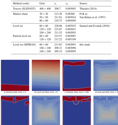
Table 1. Table containing the timing and hight (maxvrms) of the first peak of our model runs and selected others from the literature.
Method (code) Grid t1 v1 Source
Tracers (ELEFANT) 400×400 208.7 0.003093 Thieulot (2014)
Marker chain 30×30 213.38 0.00300 PvK in
50×50 211.81 0.003016 Van Keken et al. (1997)
80×80 210.75 0.003050
Level set 60×60 228.88 0.002925 Samuel and Evonuk (2010)
120×120 215.87 0.003051
240×240 211.52 0.003093
Particle level set 60×60 215.57 0.003087
120×120 212.22 0.003109
Level set (SEPRAN) 60×60 213.03 0.003091 this study
160×160 209.21 0.003096
240×240 209.19 0.003095
a) Density field, time = 0 b) Level set field, time = 0 c) Density field, time = 500 d) level set field, time = 500
e) Density field, time = 1000 f) level set field, time = 1000 g) Density field, time = 1500 h) level set field, time = 1500
Figure 2. Snapshots of the evolution of the density field and the level set field with time. Level set isocontours are plotted every 0.1. The
thick white line represents 0.
be compared with Fig. 2 from Van Keken et al. (1997). All the large-scale features (the two upwellings, the major down-wellings) are captured as well as the smaller-scale features such as the small wavelet just behind the front of the first up-welling (Fig. 2c and d). The evolution of the level set field il-lustrates the signed distance quality of the function. In Fig. 3a the root mean square velocity (vrms) of the entire domain is plotted vs. time. The first peak corresponds to the first up-welling and the second smaller peak to the second upup-welling. The figure shows the results of four of our models as well as results from the marker chain method from Van Keken et al. (1997). Figure 3c shows a close-up of the first peak. This close-up shows that our results are in good agreement with
0 0.001 0.002 0.003
0 500 1000 1500 2000
rm
s vel
ocity
(m/
s)
a) rms Velocity
60x60 diffuse boundary 160x160 diffuse boundary 240x240 diffuse boundary 160x160 sharp boundary Van Keken data (marker chain)
-2e-05 -1e-05 0 1e-05 2e-05 3e-05
0 500 1000 1500 2000
relat
ive m
ass
diffe
re
nce
time
b) relative mass difference
0.003 0.0031
200 210 220
rm
s vel
ocity
(m/
s)
time c) zoom of first peak
Figure 3. (a) Root mean square velocity of the entire domain. The Van Keken data is the data from the marker chain method of Van Keken
from the original article. (b) The relative mass difference over time according to Eq. (12). (c) A zoom-in of the first peak in the rms velocity plot of (a).
Figure 3a and c shows the results of a 160×160 sharp boundary method run and of a diffuse boundary method run. Although the overall difference is small the diffuse bound-ary method has a beneficial smoothening effect (Fig. 3c). As previously stated the signed distance quality of the level set function makes such a diffuse boundary method cheap and simple.
This benchmark involves flow of an incompressible fluid. Given the large deformation of the layers, it is appropriate to test the mass conservation of the system. To this end we calculated the relative mass difference defined in Eq. (12) and plotted the results in Fig. 3b.
Mrel=
M0−M(t ) M0
, (12)
whereM0 is the mass of the entire model domain att=0. Over time the models exhibit a variation in total mass. Att=
2000 the relative mass difference is still negligible (between 0.003 and 0.0005 %). For the higher-resolution models there is also no systematic mass variation visible. We therefore can state that our implementation of the level set method is mass conservative.
4.2 Post-glacial rebound
Crameri et al. (2012) concluded that for a correct modeling of Earth’s free surface by means of the sticky air approach
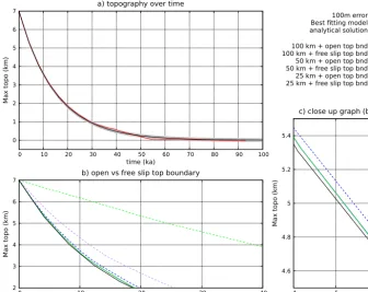
the sticky air layer should either have a 5 orders of magni-tude viscosity contrast with the underlying material and be 100 km thick or have a 4 orders viscosity contrast and be 200 km thick. In Fig. 4a we show results of a model which has a 100 km thick layer and 5 orders of magnitude difference in viscosity (ηair=1018Pa s) with the lithosphere. The gray area illustrates that the topography error of our model results never exceed 100 m. These results illustrate to our knowledge the first combination of the level set method and the sticky air approach.
0 1 2 3 4 5 6 7
0 10 20 30 40 50 60 70 80 90 100
Max topo (km)
time (ka)
a) topography over time
100m error Best fitting model analytical solution
2 3 4 5 6 7
0 10 20 30 40
Max topo (km)
time (ka)
b) open vs free slip top boundary
100 km + open top bnd 100 km + free slip top bnd 50 km + open top bnd 50 km + free slip top bnd 25 km + open top bnd 25 km + free slip top bnd
4.6 4.8 5 5.2 5.4
4 5 6
Max topo (km)
time (ka)
c) close up graph (b)
Figure 4. (a) The topography over time of our best fitting model run. (b) The data of open vs. free slip top boundaries for different sized
sticky air layers. The solid green, purple and blue line exactly overlap. Confirmed by the close-up in (c). (c) Contains a close-up of (b) showing that the three open boundary model runs (solid lines) do indeed yield exactly the same result.
a) free slip top boundary
b) open top boundary
Figure 5. Flow field in a model with a free slip top boundary (a) and
with an open top boundary (b). The arrows are scaled in the same way, both in length and color. The black line denotes the zero level set and thus the surface topography.
All thicknesses were modeled with a free slip top boundary and an open top boundary. The semi-analytical solution from Crameri et al. (2012) is plotted as well. It illustrates that with a free slip top boundary a 100 km thick (and viscosity of 5 orders lower than the lithosphere) sticky air layer is indeed needed to get satisfactory results. However, for an open top
boundary, 100, 50 and 25 km of sticky air yield exactly the same results (the graphs overlap in Fig. 4b and c). The re-sults also better match the semi-analytical solution than for 100 km sticky air and a free slip top boundary. All that is needed is a sufficiently thick sticky air layer for topography to build up. Topography variation on Earth rarely exceeds 10 km for which a sticky air layer of 25 km is by far suffi-cient and a further reduction in thickness is probably possi-ble. Assuming constant resolution a removal of 75 km of air in a 800 km high model amounts to an approximate 10 % re-duction in the number of elements. Further, as the red arrows illustrate in Fig. 5, the velocities with a free slip boundary are much larger in the air than for an open boundary. For an open boundary the time step (determined by CFL (Courant-Friedrichs-Lewy)) can thus be larger.
4.3 Subduction benchmark
200
300
400
500
600
700
0 20 40 60 80 100
d
ep
th
sla
b
ti
p
(km)
time (Myr) Depth of the tip of the slab
SEPRAN 720x180 I2ELVIS 561x141 arith ELEFANT (1000x250) arith
200
300
400
500
600
700
0 20 40 60 80 100
d
ep
th
sla
b
ti
p
(km)
time (Myr)
Depth of the tip of the slab SEPRAN 720x180 I2ELVIS 561x141 harm I2VIS 1821x93 (loc) harm I2VIS 1821x93 (loc) geom FDCON 561x141 geom I2ELVIS 884x125 (loc) arith FDCON 561x141 arith
a)
e) t = 100 Myr c) t = 40 Myr
d) t = 80 Myr b) t = 0 Myr
Figure 6. (a) Depth of slab tip vs. time. (b) through (e) snapshots in time of the slab. The red line indicates the location of the zero isocontour
of the level set function tracking the surface and the black line indicates the zero isocontour of the level set function tracking the slab.
a) current level set method b) tracer based method
entrainment of air forming a continuous layer
no entrainment of air
Figure 7. Comparison of the entrainment of air between a tracer-based method (ELEFANT) and our level set method.
Sect. 2) for viscosity can best be compared with the geomet-ric averaging method for tracers. Figure 6a shows that our slab sinks a little slower than the geometric averaging mod-els. The averaging of viscosity is especially important for large viscosity contrasts of which there are two in the mod-els of Schmeling et al. (2008): the air–slab interface and the small entrained air layer in the subduction zone (Figs. 7b and 9 of Schmeling et al., 2008). Both zones are important for the subduction velocity, the air–slab interface determines the decoupling between the two zones while a small entrained layer of air has a lubricating effect in the subduction zone. In our model the decoupling between slab and air is the same, but Fig. 7a illustrates that in our model due to the use of the level set method there is no entrainment of air and therefore no artificial lubrication of the subduction zone. This explains
why the sinking slab in our models is slightly slower than the geometric averaging model results from Schmeling et al. (2008).
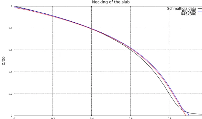
4.4 Slab detachment
0 0.2 0.4 0.6 0.8 1
0 0.2 0.4 0.6 0.8 1
D/D0
t/tc
Necking of the slab
Schmalholz data 300x200 445x300
Figure 8. The necking instability over time.
e) t = 19.3 Myr f) t = 20.5 Myr g) t = 21.7 Myr h) t = 22.8 Myr
b) t = 5.8 Myr c) t = 11.4 Myr d) t = 17.1 Myr
a) t = 0 Myr Viscosity
1E21 1E25
Figure 9. Snapshots of viscosity during the necking process. The white line indicates the zero isocontour of the level set function. Note that
the frames are plotted with different time intervals to demonstrate the acceleration of slab necking.
slab necking is that the moment the zero level set splits into two, disjoint domains can be used as a determination of the time of detachment. This was not determined by Schmalholz (2011). Figure 9 shows the time evolution of the necking process where acceleration of the process can readily be ob-served. In the first 17 Myr roughly half of the necking occurs while in the next 5 Myr it is completely detached. In the fig-ures the thick white line represents the zero isocontour of the level set function. It is important to note that although the lithosphere has broken into two disjoint domains, it is still described by a single level set function. Using the data from Fig. 8 we can time the moment of detachment at 20.4 Myr.
5 Discussion and conclusions
The level set method is not often used in geodynamical mod-eling. To investigate its applicability and benefits we have
conducted four benchmarks highlighting different aspects of geodynamical multi-material flow modeling.
local finiteelement resolution. All benchmarks thus demon-strate the level set method to be accurate.
In several cases we demonstrate favorable properties of the level set method compared to tracer-based methods. In the subduction benchmark we have shown that the level set method prevents entrainment of air into the subduction channel which otherwise would artificially lubricate the sub-duction zone. In the slab detachment benchmark we have demonstrated that the level set method can split from one bounded region into two bounded regions and accurately record the moment of detachment. In the post-glacial re-bound benchmark we illustrated that we match the semi-analytical solution using similar elemental resolutions as tracer-based methods. This further illustrates the statement of Zlotnik et al. (2008) that the level set method is favorable, particularly for 3-D applications, to the tracer method with regard to computational costs.
The level set function is chosen to be a signed distance function. This makes the implementation of a diffuse bound-ary method (Eq. 8) simple and the boundbound-ary width (h) easily adjustable. In the Rayleigh–Taylor instability benchmark we have shown that such a diffuse boundary method has a sta-bilizing effect on the results but does not alter them in any significant way.
With the post-glacial rebound benchmark we demon-strated that the thickness of the sticky air layer can be re-duced significantly when using a zero stress, free through-flow open top boundary resulting in an even better fit with the semi-analytical solution.
Overall we have shown that the level set method performs well and occasionally even better in geodynamical multi-material flow benchmarks and could therefore be considered as an alternative for tracer-based and phase field methods. For 3-D applications one can add to this the lower computa-tional costs compared to tracer-based methods (Zlotnik et al., 2008).
Acknowledgements. We would like to thank Peter Van Keken, Stephan Schmalholz, Fabio Crameri and Haro Schmeling for the fast sharing of data used in this paper. We thank two anonymous reviewers for their constructive comments that helped to improve our paper. We acknowledge the Netherlands Research Institute of Integrated Solid Earth Sciences (ISES) for research funding and funding of computational support. This work was partly supported by the Research Council of Norway through its Centres of Excellence funding scheme, project number 223272.
Edited by: T. Gerya
References
Adalsteinsson, D., and Sethian, J.: The Fast Construction of Ex-tension Velocities in Level Set Methods, J. Comput. Phys., 148, 2–22, 1999.
Andrews, E. and Billen, M.: Rheologic controls on the dynamics of slab detachment, Tectonophysics, 464, 60–69, 2009.
Androviˇcová, A., ˇCižková, H., and van den Berg, A.: The effects of
rheological decoupling on slab deformation in the Earth’s upper mantle, Stud. Geophys. Geod., 57, 460–481, 2013.
Bangerth, W. and Heister, T.: ASPECT: Advanced Solver for Problems in Earth’s ConvecTion, Texas A&M Univer-sity/Computational Infrastructure in Geodynamics, 2013. Baumann, C., Gerya, T., and Connolly, J.: Numerical modelling of
spontaneous slab breakoff dynamics during continental collision, Geological Society, London, Spec. Publicat., 332, 99–114, 2010.
Bˇehounková, M. and ˇCižková, H.: Long-wavelength character of
subducted slabs in the lower mantle, Earth Planet. Sc. Lett., 275, 43–53, 2008.
Billen, M. and Hirth, G.: Rheologic controls on slab
dynamics, Geochem. Geophy. Geosy., 8, Q08012,
doi:10.1029/2007GC001597, 2007.
Bourgouin, L., Mühlhaus, H.-B., Hale, A., and Arsac, A.: Towards realistic simulations of lava dome growth using the level set method, Acta Geotech. Slov., 1, 225–236, 2006.
Bourgouin, L., Mühlhaus, H.-B., Hale, A., and Arsac, A.: Studying the influence of a solid shell on lava dome growth and evolution using the level set method, Geophys. J. Int., 170, 1431–1438, 2007.
Braun, J., Thieulot, C., Fullsack, P., DeKool, M., Beaumont, C., and Huismans, R.: DOUAR: a new three-dimensional creeping flow numerical model for the solution of geological problems, Phys. Earth Planet. In., 171, 76–91, 2008.
Brooks, A. and Hughes, T.: Stream-line upwind/Petrov–Galerkin formulation for convection dominated flows with particular em-phasis on the incompressible Navier–Stokes equations, Comput. Methods Appl. Mech. Engrg., 32, 199–259, 1982.
Chertova, M. V., Geenen, T., van den Berg, A., and Spakman, W.: Using open sidewalls for modelling self-consistent lithosphere subduction dynamics, Solid Earth, 3, 313–326, doi:10.5194/se-3-313-2012, 2012.
Christensen, U.: The influence of trench migration on slab penetra-tion into the lower mantle, Earth Planet. Sc. Lett., 140, 27–39, 1996.
Chopp, D.: Another look at velocity extensions in the level set method, SIAM J. Sci. Comput., 31, 3255–3273, 2009.
ˇ
Cížková, H., van Hunen, J., and van den Berg, A.: Stress distribution within subducting slabs and their deformation in the transition zone, Phys. Earth Planet. In., 161, 202–214, 2007.
Crameri, F., Schmeling, H., Golabek, G., Duretz, T., Orendt, R., Buiter, S., May, D. A., Kaus, B., Gerya, T., and Tackley, P.: A comparison of numerical surface topography calculations in geodynamic modelling: an evaluation of the “sticky air” method, Geophys. J. Int., 189, 38–54, 2012.
Duan, X., Ma, Y., and Zhang, R.: Optimal shape control of fluid flow using variational level set method, Phys. Lett. A, 372, 1374–1379, 2008.
Duretz, T., Gerya, T., and May, D.: Numerical modelling of spon-taneous slab breakoff and subsequent topographic response, Tectonophysics, 502, 244–256, 2011.
Duretz, T., Gerya, T. V., and Spakman, W.: Slab detachment in lat-erally varying subduction zones: 3-D numerical modeling, Geo-phys. Res. Lett., 41, 1951–1956, 2014.
Enright, D., Fedkiw, R., Ferziger, J., and Mitchell, I.: A Hybrid Particle Level Set Method for Improved Interface Capturing, J. Comput. Phys., 183, 83–116, 2002.
Fullsack, P.: An arbitrary Lagrangian-Eulerian formulation for creeping flows and its application in tectonic models, Geophys. J. Int., 120, 1–23, 1995.
Fedkiw, R., Aslam, T., Merriman, B., and Osher, S.: A non-oscillatory Eulerian Approach to Interfaces in Multimaterial Flows (the Ghost Fluid Method), J. Comput. Phys., 152, 457–492, 1999.
Gerya, T., Fossati, D., Cantieni, C., and Seward, D.: Dynamic ef-fects of aseismic ridge subduction: numerical modelling, Eur. J. Mineral., 21, 649–661, 2009.
Gottlieb, S. and Shu, C.: Total variation diminishing Runge–Kutta schemes, Math. Comput., 67, 73–85, 1998.
Gross, L., Bourgouin, L., Hale, A., and Mühlhaus, H.-B.: Interface modeling in incompressible media using level sets in Escript, Phys. Earth Planet. In., 163, 23–34, 2007.
Gurnis, M. and Hager, B.: Controls of the structure of subducted slabs, Nature, 335, 317–321, 1988.
Hale, A., Bourgouin, L., and Mühlhaus, H.: Using the level set method to model endogenous lava dome growth, J. Geophys. Res., 112, B03213, doi:10.1029/2006JB004445, 2007.
Hale, A., Gottschaldt, K., Rosenbaum, G., Bourgouin, L., Bauchy, M., and Mühlhaus, H.: Dynamics of slab tear faults: in-sights from numerical modelling, Tectonophysics, 483, 58–70, 2010.
Jiang, G. and Peng, D.: Weighted ENO schemes for Hamil-ton–Jacobi equations, SIAM J. Sci. Comput., 21, 2126–2143, 2000.
Kronbichler, M., Heister, T., and Bangerth, W.: High accuracy man-tle convection simulation through modern numerical methods, Geophys. J. Int., 191, 12–29, 2012.
Lenardic, A. and Kaula, W.: A numerical treatment of geodynamic viscous flow problems involving the advection of material inter-faces, J. Geophys. Res., 98, 8243–8260, 1993.
Magni, V., van Hunen, J., Funiciello, F., and Faccenna, C.: Numeri-cal models of slab migration in continental collision zones, Solid Earth, 3, 293–306, doi:10.5194/se-3-293-2012, 2012.
Min, C.: On reinitializing level set functions, J. Comput. Phys., 229, 2764–2772, 2010.
Oka, H. and Ishii, K.: Numerical analysis on the motion of gas bubbles using level set method, J. Phys. Soc. Jpn., 68, 823–832, 1999.
Osher, S. and Fedkiw, R.: Level set methods: an overview and some recent results, J. Comput. Phys., 169, 463–502, 2001.
Osher, S. and Sethian, J.: Fronts propagating with curvature-dependent speed: algorithms based on Hamilton-Jacobi formu-lations, J. Comput. Phys., 79, 12–49, 1988.
Osher, S. and Shu, C.-W.: High-order essentially non-oscillatory schemes for Hamilton–Jacobi equations, SIAM J. Numer. Anal., 28, 907–922, 1991.
Quinquis, M., Buiter, S., and Ellis, S.: The role of boundary conditions in numerical models of subduction zone dynamics, Tectonophysics, 497, 57–70, 2011.
Rao, R., Mondy, L., Noble, D., Moffat, H., D. B., A., and Notz, P.: A level set method to study foam processing: a validation study, Int. J. Numer. Meth. Fl., 68, 1362–1392, 2011.
Samuel, H. and Evonuk, M.: Modeling advection in geophysical flows with particle level sets, Geochem. Geophy. Geosy., 11, Q08020, doi:10.1029/2010GC003081, 2010.
Schmalholz, S.: A simple analytical solution for slab detachment, Earth Planet. Sc. Lett., 304, 45–54, 2011.
Schmeling, H., Babeyko, A., Enns, A., Faccenna, C., Funiciello, F., Gerya, T., Golabek, G., Grigull, S., Kaus, B., and Morra, G.: A benchmark comparison of spontaneous subduction models – towards a free surface, Phys. Earth Planet. In., 171, 198–223, 2008.
Segal, A. and Praagman, N.: The SEPRAN package. Technical re-port, Technical, Ingenieurs-Bureau Sepra, the Netherlands, avail-able at: http://ta.twi.tudelft.nl/sepran/sepran.html, 2005. Sethian, J.: Evolution, Implementation and Application of Level Set
and Fast Marching Methods for Advancing Fronts, J. Comput. Phys., 169, 503–555, 2001.
Suckale, J., Hager, B., Elkins-Tanton, L., and Nave, J.: It takes three to tango: 2. Bubble dynamics in basaltic volcanoes and ramifi-cations for modeling normal Strombolian activity, J. Geophys. Res., 115, B07410, doi:10.1029/2009JB006917, 2010.
Sussman, M., Fatemi, E., Smereka, P., and Osher, S.: A level set approach for computing solutions to incompressible two-phase flow II, in: Proceedings of the Sixth International Symposium on Computational Fluid Dynamics, Lake Tahoe, NV, 1995. Tackley, P. and King, S.: Testing the tracer ratio method
for modeling active compositional fields in mantle con-vection simulations, Geochem. Geophy. Geosy., 4, 8302, doi:10.1029/2001GC000214, 2003.
Thieulot, C.: FANTOM: two- and three-dimensional numerical modelling of creeping flows for the solution of geological prob-lems, Phys. Earth Planet. In., 188, 47–68, 2011.
Thieulot, C.: ELEFANT: a user-friendly multipurpose geodynam-ics code, Solid Earth Discuss., 6, 1949–2096, doi:10.5194/sed-6-1949-2014, 2014.
Thieulot, C., Glerum, A., Hillebrand, B., Spakman, W., and Torsvik, T.: Multiphase geodynamical modelling using Aspect, in preparation, 2014a.
Thieulot, C., Schmalholz, S., Glerum, A., Hillebrand, B., and Spak-man, W.: A two- and three-dimensional numerical comparison study of slab detachment, in preparation, 2014b.
van Hunen, J. and Allen, M.: Continental collision and slab break-off: a comparison of 3-D numerical models with observations, Earth Planet. Sc. Lett., 302, 21–37, 2011.
van Hunen, J. and van den Berg, A.: Plate tectonics on the early Earth: limitations imposed by strength and buoyancy of sub-ducted lithosphere, Lithos, 103, 217–235, 2008.
Van Keken, P., King, S., Schmeling, H., Christensen, U., Neumeis-ter, D., and Doin, M.: A comparison of methods for the modeling of thermochemical convection, J. Geophys. Res.-Sol. Ea., 102, 22477–22495, 1997.
van der Pijl, S., Segal, A., Vuik, C., and Wesseling, P.: Computing three-dimensional two-phase flows with a mass-conserving level set method, Comput. Visual, Sci., 11, 221–235, 2008.