Multi-sensor Data Fusion Based on Consistency Test and Sliding Window Variance Weighted Algorithm in Sensor Networks

(1)

Multi-sensor Data Fusion Based on Consistency

Test and Sliding Window Variance Weighted

Algorithm in Sensor Networks

Jian Shu1,2, Ming Hong1,3, Wei Zheng1,3, Li-Min Sun2,4, and Xu Ge1,3

1_{Internet of Things Technology Institute, Nanchang Hang Kong University,}

Nanchang China [email protected]

2_{School of Software, Nanchang Hang Kong University,}

3_{School of Information Engineering, Nanchang Hang Kong University,}

4_{Institute of Software Chinese Academy of Science,}

Abstract. In order to solve the problem that the accuracy of sensor data is reducing due to zero offset and the stability is decreasing in wireless sensor networks, a novel algorithm is proposed based on consistency test and sliding-windowed variance weighted. The internal noise is considered to be the main factor of the problem in this paper. And we can use consistency test method to diagnose whether the mean of sensor data is offset. So the abnormal data is amended or removed. Then, the result of fused data can be calculated by using sliding window variance weighted algorithm according to normal and amended data. Simulation results show that the misdiagnosis rate of the abnormal data can be reduced to 3% by using improved consistency test with the threshold set to [0.05, 0.15], so the abnormal sensor data can be diagnosed more accurately and the stability can be increased. The accuracy of the fused data can be improved effectively when the window length is set to 2. Under the condition that the abnormal sensor data has been amended or removed, the proposed algorithm has better performances on precision compared with other existing algorithms.

(2)

1.

Introduction

Wireless sensor network (WSN) which is constituted by a large number of micro-sensor nodes deployed in the monitored area can sense, collect, and process the information of monitored objects in the coverage area. Then the processed data is sent to the observer through the multi-hop self-organized

network [1]. Since the nodes are generally battery-powered and deployed in a

harsh environment area, some of which are not available for human, it’s unrealistic to replace battery for continuous power supply. The nodes will die as long as the energy is drained out. The network may work abnormal or even failure once some nodes are dead. Moreover, the external noises and internal noises can affect the accuracy of the sensor data. The external noises include electromagnetic radiation, temperature and pressures, and internal noises include the decrease of stability and the zero offset in some sensors which have been used for a long time. With the help of multi-sensor data fusion algorithms, the precision of data can be improved.

In order to solve the problem that the precision of data fusion is low due to zero drift and the drop of the stability for part of the sensor when multiple sensor nodes measuring on the same target. This paper introduces a multi-sensor data fusion method based on consistency test and sliding-windowed variance weighted in sensor networks. Firstly, we propose a sensor measurement model, and the model can simplify the core problem to the result of internal noise. Then we present a consistency test with the new confidence distance to diagnose whether the mean of internal noise is shift under the sliding window mode, so that the abnormal sensor which will lead to zero drift can be amended or removed conditionally. Finally, we make data fusion processing of the normal sensors measured value and some certain amended abnormal sensors by sliding window sample variance weighted method, so that more precise data can be obtained.

2.

Related Studies

Data fusion in WSN is different from traditional ones since the ability of node is limited. Nodes are battery-powered, the ability of CPU is weak, and wireless communication is unstable. Therefore, Traditional complex and high energy-consuming fusion algorithms are not suitable for WSN. There exist

some algorithms, such as weighted average algorithm, Kalman Filter [2] and

Bayes estimation [3] to solve the problem.

(3)

Weighted Algorithm in Sensor Networks

calculating the sample mean and the sample variance of each batch. Adaptive variance-weighted method is proposed in literature [6] under the premise that external noise is stable. it is proposed to solve the problem that the variance of each sensor is unknown with the help of the variance of sample. Iteration method is used to aggregate multi-sensor data in literature [7], it is based on adaptive variance weighted algorithm. And the result shows that good precision can be obtained. Literature [8] adopts window variance weighted algorithm in this direction and illustrate its idea on window size definition according to different noise change. In regard to the characteristics of sensor noise abruption, Literature [9] proposed the variance weighted algorithm based on adaptive window length. It divided noise estimate curve into smooth zone and abrupt zone by detecting noise change in sensor data, meanwhile it uses corresponding window size to revise multi-sensor fusion value and improves final aggregating accuracy according to different curve level.

Consistency test method focuses on the problem that there will be a deviation when various types of sensors measuring on the same target, it tests and removes the sensor with larger deviation to reduce the impact on fusion. Nowadays there are mainly some consistency test methods based on relation matrix and distribution graph, and according to how to determine the relation matrix, the former method which is based on relation matrix can be divided into three parts:1. It is a consistency test method based on relation

matrix which is determined by the confidence matrix[10], which is established

on known measurement model and noise as the Gaussian noise, the relation matrix is obtained by calculating the confidence distance between each two nodes, and then, this method tests the sampling value with larger deviation by graph theory approach;2.It is a consistency test method based on relation

matrix which is determined by degree of support[11].Based on the

measurement model, this method quantifies the support degree of the measured value of each two sensors by an exponential decay function. And determines the sampling value with larger deviation by the experience threshold value; 3. It is a consistency test method based on relation matrix

which is determined by statistic distance [12], the method is still established on

known measurement model and noise as the Gaussian noise, defines the statistic distance of observations of each two sensors based on the multivariate normal distribution to determine the relation matrix, and obtains sensor set with the biggest mutually support through directed graph theory; 4. It is a consistency test method based on relation matrix which is determined

by empirical threshold [13], the method determines the trust degree of

observations of each two sensors by the curve function with a empirical threshold to obtain the relation matrix, and determines the weight of each sensor observations by the largest eigenvector of the matrix, finally makes the fusion processing. Relying on Moffat distance to define relational matrix,

the consistency check approach [14] uses Moffat and involving criterions to

(4)

3.

System Model

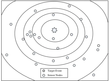
In wireless sensor network, as show in Fig.1, there are discrepancies of the values on the same target measured by different sensors because of the affection from noises. The noises include external noise and internal noise.

Target Event Sensor Nodes

Fig. 1. A example of Sensor Nodes Deployment.

External noise is mainly caused by environment change which includes temperature, pressure and electromagnetic radiation. And we use Gaussian white noise which is zero mean value and different variance in the model definition period.

Internal noise is mainly caused by the sensors themselves. It is relatively stabilized, and it is not changed in a short period. For example, there exists zero offset because of shedding of element wiring, burn-in and similar factors. It is usually using Gaussian white noise which is nonzero mean value and constant variance in the model definition period. The zero drift phenomena are assumed as the measured values of some sensors are smaller or larger than normal ones. The decreasing stability of sensors is showed as the large undulatory property of the measured values.

Literature [15] proposes a sensor measuring model

z



x





and a noise

model~N(0,1). Considering the change of both external noise and the

inconsistency of noise among different sensors, a new sensor measuring model is shown as formula (1).

i

k

x

k

z

(

)



(

)





(

)





(1)

)

(

k

z

_i is the

k



th

measured value of sensor i.

x

(

k

)

is the

k



th

real value

of target object, and it is a constant if

k

is given . ( )~ (0, 2( ))

k N

k 

 is the

k



th

external noise, it is changed with times. i~N(i,i2) is the internal

(5)

Assuming that external noise and internal noise are mutual independent, the measuring model can be simplified as formula (2).

)

(

)

(

)

(

k

x

k

z

_i







_i (2)

) ) ( , ( ~ )

( _i 2 _i2

i k N   k 

  is integrated noise.

It is supposed that n sensors measure a same target simultaneously. Each

sensor contains a sliding window whose length is W for storing sampling

values in the first W times. The

k



th

measured value of sensor i is z_i(k).

The sliding window’s sample mean isz_i(k) and its sample variance is *2( )

k

S_i .

4.

Multi-sensor Data Fusion Based on Consistency Test

and Sliding Window Variance Weighted Algorithm in

Sensor Networks

4.1. The traditional consistency test algorithm

Luo and his assistants proposed a consistency test to solve the problem of inconsistence of measured value from the sensors which measure on the same target. Based on the sensor measuring model which is established in this algorithm, the error sensor data is removed after calculating the confidence distance of each two sensors and establishing the relationship matrix between the sensors, and then the optimal statistical decision making methods are used for fusion.

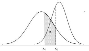
Confidence Distance [10]: There are n sensors which measure the same

target, and the measured data of all sensors

x

₁,

x

₂, ...,

x

_n can be obtained, if

1

x

follows Gaussian distribution and the corresponding density function is

( )

i x

P

. The confidence distance can be obtained by formula (3).

A dx x x P

d i

j x

x i i

ij 2



( | ) 2 (3)

    

  

        

2

2 1 exp 2 1 ) | (

i i i

i

x x x

x P

 

(4)

Where

d

_ij in the formula (3) represents for the confidence distance

between sensor i and sensor j,



_iis the variance of sensor i, A is the area

enclosed by the conditional probability density curve,

x



x

_i,

x



x

_j and

x

(6)

xi xj

A

Fig. 2. The schematic diagram of confidence distance.

The smaller the value of

d

_ij is, the closer value of sensor i to sensor j is.

In order to simplify the calculation, Luo has introduced the error function

(5), and

d

_ij is shown as formula (6).

dz z erf 



 

  0 2 ) exp( 2 )

( (5)

) 2 ( i i j ij x x erf d  

 (6)

Confidence distance matrix [10]: The confidence distances of each two

sensors can be obtained. They constitute the

n n



matrix defined as the

confidence distance matrixD_{n n}_ .

              nn n n n n n n d d d d d d d d d D        2 1 1 22 21 1 12 11 (7)

Relation Matrix [10]: Since the threshold

d

_ijis given, the relationship value

of each two sensors can be calculated by formula (8). We constitute the

n n



matrix defined as the relation matrixR_{n n} .

) ,..., 2 , 1 , ( 0 1 n j i d d r ij ij ij ij ij        

 ₍₈₎

              nn n n n n n n r r r r r r r r r R        2 1 1 22 21 1 12 11 (9)

In the relation matrixR_{n n}_ ,

r

_ij represents for the support degree of the

(7)

have any relationship. When one of

r

_ij and

r

_ji equals 0 and another equals

1, it means that the relationship between them is weak. If r_ij r_ji1, it

means that sensor i and sensor j have a strong relationship. Thus, the largest

supported sensor set is obtained through the relation matrix, and then the optimal estimation methods are used for the last aggregation.

But there are several problems to be solved in wireless sensor networks:

1) According to the confidence distance from formula (5), each sensor's

variance is need to be given for the calculation of confidence distance of each two sensors, it is can be described by integrated noise

variance 2 2

) (k i

  , but it can be obtained in wireless sensor networks.

So it is not suitable.

2) Since the confidence distance from formula (5) and (6) contains

integral calculation, the calculation is so complex that it is not suitable in wireless sensor network.

3) The method doesn’t propose a approach how to get the largest

supported sensor set.

Therefore, we make the following improvements on the algorithm.

4.2. A new definition of confidence distance

According to formula (2), we can get the following conclusions: the difference

between the values can be obtained by the

k



th

data of sensor i and j, and

it follow the Gaussian distribution, that is

) ) ( ), ( ( ~ ) ( ) ( ) ) ( ), ( ( ~ ) ( ) ( 2 2 2 2 j j j i i i k k N k x k z k k N k x k z         

 ₍₁₀₎

The problem which is to judge whether one of sensor i or j incur zero offset

can be transformed into the problem of the hypothesis testing of the mean difference for two samples of normal distribution:

0 ) ( ) ( : 0 ) ( ) ( : 1 0     k k H k k H j i j i   

 ₍₁₁₎

Under the significance level



, the test statistic T is obtained.

2 / 1 2 2 2

2 ₍₎

) ( 0 ] ) ( ) ( ) ( ) ( [                u n k n k k x k z k x k z T j j i i j i (12)

)

(

k

(8)

2 / 1 2 2 2 2₍ ₎ ₍ ₎

0 )] ( ) ( [              u n k n k k z k z T j j i i j i (13)

If the test statistic T meets the conditions, we can reject the hypothesis

H

₀,

it represents that there is a large difference between sensor i and j, and one

of them may exist zero offset.

But the external noise variance 2( )

k

 and internal noise variancei2(k) of

each sensor can not be obtained, and



12(k), ( )

2 2 k

 , …,



i2(k)are not the

same in wireless sensor networks.

In order to obtain the test statistic, we introduce the conclusions of the limit distribution, a new test statistic as shown as formula (14).

2 / 1 2 * 2 * ) ( ) ( ) ( ) (       u n k S k S k z k z T j i j

i (14)

Therefore, we can define a new confidence distance as follow:

}] ) ( ) ( ) ( ) ( { 1 [ 2 2 * 2 * n k S k S k z k z x P d d j i j i ji ij         (15)

Where

d

_ijis the significance level of the hypothesis testing, according to

the consequences of committing two type errors, when the value of



is

small, the probability of error type II increases accordingly, that is it will be easy to make substandard products in the test sample judged to be qualified,

then to accept the original hypothesis. If the value of



is large, the

probability of error type I increases, so it is easy to make qualified products in the test sample is deemed to have failed and then to be refused. Considering that the abnormal sensor have much great impact on fusion, we need to minimize the probability of error type II, that means we should try our best to prevent abnormal sensors judged to be normal ones. Therefore, the larger

the value of

d

_ij is, the less obvious the mean integrated noise of sensor i and

j is. That is, sensor i and j may both belong to the normal sensors and may

also both belong to abnormal sensors.

But formula (15) can not be applied in sensor nodes because of complex calculation. Therefore it requires an easy method to calculate sensor

relational matrix directly. In order to solve the problem, the threshold



₀of

(9)

2 / 1 2 * 2

* 0

) ( ) (

 

   

 u

n k S k S

k z k z T T

window j i

j i ji ij

(16)

In corresponding to relational matrix factor

r

_ij



r

_ji



0

,otherwise,

1

ij ji

r



r



. In this way, it can avoid complex calculation and reduce energy

consumption.

4.3. The diagnosis of abnormal sensors

According to the new definition of confidence distance, the confidence

matrixD_n_n is obtained, and the relation matrix Rnn is also obtained.

Relation matrix n n

R is a symmetric matrix composed by 0 and 1.

0

ij ji

r



r



represents that the mean integrated noise of sensor i is much

different from sensor j, therefore, one of the sensors must be a abnormal

sensor.

r

_ij



r

_ji



1

represents that the mean integrated noise of sensor i is

less different from sensor j, that’s they may be both normal or abnormal.

Assuming the sensor node is the vertexes of graph G and relational matrix

n n

R is the adjacency matrix of graph G, hereby, we could plot the entire

correlation graph of all sensor nodes. According to theory of resolving

maximum clique G’ of graph G[16]_{, the vertexes of clique G’ composed}

normal sensor group A, and the remaining of them composed abnormal sensor group B. In order to avoid judging mistakenly, it is necessary to make sure the percentage of normal sensors is beyond 50%. Otherwise, it is possible to make a wrong judgment.

Algorithm 1: program for Max Clique

MaxClique(G; size)

if |G|=0 then

if size>max then

max:=size

New record; save it.

end if

return

end if

while G !=0 do

(10)

return

end if

i:=min{j | vj ∈G}

G:=G\{vi}

MaxClique(G ∩ N(vi); size +1)

end while

return

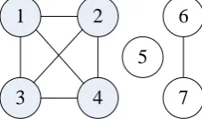
Fig. 3 is the relationship diagram G showing the degree of support of 1-7 sensors, in which node 1, node 2, node 3 and node 4 constitute the maximum clique G’. Therefore, we can determine that node 1, node 2, node 3 and node 4 constitute the normal sensor set, and node 5, node 6, and node 7 constitute the abnormal sensor set.

1

3

4

2

7

5

6

Fig. 3. The diagram of the degree of support for each sensor.

4.4. The sliding window variance weighted algorithm and how to amend or remove the measured data from abnormal sensors

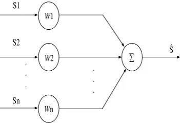
The fundamental principle of adaptive weighted algorithm: under the condition of minimum average variance, it can find the best corresponding

weight W_iof each sensor node with an adaptive way, and help Sˆ achieve the

best fusion result. As.0 Fig.4 shows, S_i is the measure value of sensor

nodes, where i=1,2…,n, while Sˆ is the final fusion result.

According to this theory, the sliding window variance weighted algorithm:

In wireless sensor networks, since the external noise variance 2( )

k

 and the

internal noise variance 2₍ ₎

k

i

 of the

k



th

measurement of sensors carried

by each sensor node are unknown. In order to solve this problem, the sample variance can be used to replace real variance, the weight of each sensor data can be obtained by formula (17).





 _n

j j i i

k S

k S W

1 2 * 2 *

) ( / 1

) ( /

(11)

Weighted Algorithm in Sensor Networks S1

S2

Sn W1

W2

Wn

∑ Ŝ

. . .

Fig. 4. Model of adaptive weighted estimate fusion.

Algorithm 2: program for sample variance

while(n<WINDOW_NUM) do

if(Position<Size) then

AVE average value

if(position=0) then

VAR=0; variance=0

else caculate VAR

New record; save it.

end if

else if(Position=Size) then

caculate AVE

caculate VAR

end if

end while

return

Algorithm 3: program for sliding-window weight and fusion value

while(n<NODE_NUM) do

if(G.pNode!=0)

update SensorValue

update SensorWeight

(12)

else if(G.pNode!=0&&Node[i].VAR<Node[j].VAR)

update SensorValue

update SensorWeight

end if

end while

How to amend or remove the measured data from abnormal sensors: if the

greatest normal sensor set A and abnormal sensor set B are obtained, we

amend or remove under certain conditions:

1) SensormB, if



sensor

n



A

, and *2 *2

( ) ( )

m n

S k S k , z_m(k) is needed

to be amended by using formula (18), (19) and (20).

m m

m k z k

z ( ) ( ) (18)





  

A i

i i m

m z (k) wz (k) (19)







A j

j i i

k S

k S w

) ( / 1

2 * 2 *

(20)

2) SensormB , ifsensor

n



A

, there is *2 *2

( ) ( )

m n

S k S k , z_m(k)is needed to be removed simply.

5.

Simulation Research

In order to verify the validity of the algorithm, OMNet++ is used for simulation. According to the experimental results obtained under different

significance level threshold



₀ and the length of window W, the optimal value

best



and Wbest can be evaluated. Then the precision of algorithm is compared

with three other fusion algorithms such as arithmetic average algorithm, batch estimation algorithm and the adaptive variance weighted algorithm. Cluster-based routing protocol is used in the experiment, each cluster has 41 nodes (including one cluster head), and the cluster head takes responsible for data fusion. The sliding window length of the member nodes is set to W, and

significance level threshold is



₀.

According to the model that z_i(k)x(k)(k)_i.Gaussian white noise

whose mean is zero is used for simulating the external noise(k), and its

variance will change every R_ times. Internal noise



_i can be described by

(13)

sensor node is P, it assumes that the internal noise is stable, and will not change as time changes. Considering the changing characteristic of the

target object’s actual value, x(k) is generated randomly and changes

everyR_x.

0.0025 0.01 0.05 0.15 0.25 0.35 0.45 0.55 0.65 0.75 0.85 0.95

1.5 1.75 2 2.25 2.5 2.75

Mean Square Error

2.5-2.75 2.25-2.5 2-2.25 1.75-2 1.5-1.75

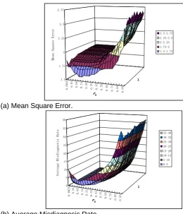
(a) Mean Square Error.

0.0025 0.01 0.05 0.15 0.25 0.35 0.45 0.55 0.65 0.75 0.85 0.95

0 5 10 15 20 25 30 35 40

Average Misdiagnosis Rate

35-40 30-35 25-30 20-25 15-20 10-15 5-10 0-5

(b) Average Misdiagnosis Rate.

Fig. 5. Simulation Results under Different Significance Level Threshold and Window Size W.

5.1. The best significance level threshold



_best

In order to obtain optimize significance level threshold



_best, the parameters

are set as follows: n=40, N=200, R_=10,P=0.3,

R

_x=10, and ₀[0,1] and

] 30 , 2 [



W . Fig. 5(a) and Fig. 5(b) illustrate the simulation results for this

experiment. The

x

-axis represents significance level threshold and the

y

(14)

the Fig. 5(a). The

z

-axis represents average misdiagnosis rate in the Fig. 5(b).

1)



₀[0,0.05], mean square error and average misdiagnosis rate

decreases rapidly when



₀ is increasing. The higher the value of



₀,

the lower the probability of Error-type-I is, it means that the normal sensor nodes have less probability to be diagnosed as abnormal nodes.

2)



₀[0.05,0.15], mean square error and average misdiagnosis rate

tend to be stationary. The reason is that when



₀ changed within the

range, all the abnormal sensors are diagnosed correctly, it has less effect on mean square error and average misdiagnosis rate.

3)



₀[0.15,1], mean square error and average misdiagnosis rate

increases rapidly as



₀ is increasing. The higher the value of



₀, the

higher the probability of Error-type-II is. It means that the abnormal nodes can be mistakenly diagnosed as normal nodes easily.

Therefore, the optimal range of significance level threshold



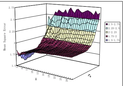
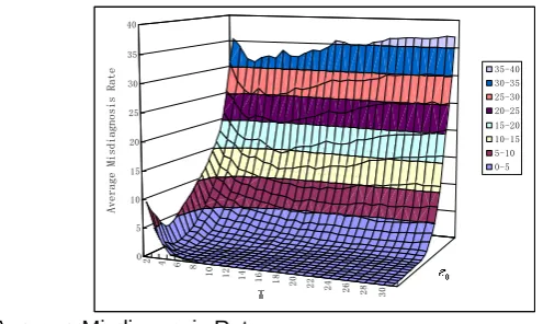
₀ is [0.05, 0.15].

5.2. The best window size Wbest

Similarly, in order to obtain the optimistic window size Wbest，Fig. 6(a) and

Fig. 6(b) illustrate the simulation results for this experiment. The

x

-axis

represents window size and the

y

-axis represents significance level

threshold. The

z

-axis represents mean square error in the Fig. 6(a). The

z

-axis represents average misdiagnosis rate in the Fig. 6(b).

1 ₄

7

10 ₁₃ 16 ₁₉

22 ₂₅

28

1.5 1.75 2 2.25 2.5 2.75

Mean Square Error

2.5-2.75 2.25-2.5 2-2.25 1.75-2 1.5-1.75

(15)

2 4 6 8

10 12 14 16 18 20 22 24 26 28 30

0 5 10 15 20 25 30 35 40

Average Misdiagnosis Rate

35-40 30-35 25-30 20-25 15-20 10-15 5-10 0-5

(b) Average Misdiagnosis Rate.

Fig. 6. Simulation Results under Different Significance Level Threshold and Window Size W.

According to Fig. 6, the mean square error increases with the increment of window size, but the average misdiagnosis rate increases little. Thus, it is clear that window size W only have impact on the mean square error.

1) W[2,10]，the mean square error rises sharply. Because the window

size is in the range of

R

_x and

R

_. The larger window size is, The

lower fusion accuracy is.

2) W[10,30]，the mean square error rise gradually, because the

window size already exceeds both

R

_x and

R

_ . The deviation

between estimated sensor noise variance and real one reaches the highest value.

Therefore, the optimistic sliding window size Wbest=2 is obtained.

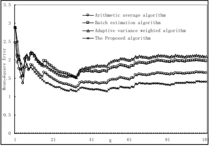
5.3. The precision comparison

Fig. 7 shows the simulation results of the proposed algorithm compared with arithmetic average algorithm, batch estimation algorithm and adaptive

variance weighted algorithm under the condition of n=30, W=Wbest=2，

N=100,



₀=



_best=0.10,R_=10,P=0.3 and

R

_x=10.

(16)

this method will make the weight too big from its possible value range, directly cause fusion precision depressing and lead to the worst fusion result.

Batched estimation algorithm only uses batching method to fuse multi-sensor data, takes the reciprocal of each sample variance as the weight and sample average value and neglects the fact that sensor nodes lacks stability. Experiment result shows that average variance tends to high which means a low data fusion outcome; and arithmetic mean algorithm improve the fusion precision compared to above two approaches by using average calculating operation that may cover those effects brought by Zero offset and low stability sensors, for the weights of sensor nodes are all equal. However, the fusion result remains undesirable for it don’t take the problems of Zero offset and stability difference into account.

Based on traditional adaptive variance weighted algorithm, our protocol uses conditional amend method to correct some of the abnormal sensor value which have a good stability, then adds them into the weighted fusion sequence of normal sensor group making the information required by data fusion large enough to enhance fusion precision. And the result appears to have minimum average variance, estimated fusion data closer to real value and best fusion performance compared to others. The reasons are shown as follows: Firstly, consistency test is used for diagnosing the abnormal sensor data; Secondly, it corrects the abnormal data in some degree. Finally, sliding window weighted algorithm is used for the last fusion.

0 0.5 1 1.5 2 2.5 3 3.5

1 21 41 K 61 81 101

Mean Square Error

Arithmetic average algorithm Batch estimation algorithm Adaptive variance weighted algorithm The Proposed algorithm

Fig. 7. The Precision Comparison using the Proposed Algorithm vs Arithmetic Average Algorithm, Batch Estimation Algorithm and Adaptive Variance Weighted Algorithm.

6.

Conclusion

(17)

and internal noise. Firstly, an improved consistency test algorithm is used for diagnosing sensor data and obtaining the normal sensor set and abnormal sensor set. Secondly, the abnormal sensor value is amended or removed under some degrees. Finally, sliding window variance weighted algorithm is proposed for the last data fusion. The simulation result shows that the optimum consistency test threshold range is [0.05, 0.15] and the optimum sliding window size is 2. The results also show that it has better performances on precision compared with other existing algorithms.

References

1. Chong C Y, Kumar S P, “Sensor networks: Evolution, opportunities and challenges,” Proceedings of the IEEE, vol. 91, pp. 1247-1256, 2003.

2. Olfati-Saber R, “Distributed Kalman filter with embedded consensus filters,” Proceedings of Conference on Joint CDC-ECC’05, Dec 2005.

3. Zhang Shu-kui, Cui Zhi-ming, Gong Sheng-rong, “A Data Fusion Algorithm Based on Bayes Sequential Estimation for Wireless Sensor Network,” Journal of Electronics & Information Technology, vol. 31, pp. 716-721, 2009.

4. Liao Xi-chun, Qiu Min, Mai Han-rong, “Study on data fusion algorithms based on parameter-estimation,” Transducer and Microsystem Technologies, vol. 25, pp. 70-73, 2006

5. Zhang Xi-liang, Sun You, “A data aggregation arithmetic based on directed diffusion and batch estimate for wireless sensor network,” Control & Automation, vol. 6, pp. 173-174,180, 2006.

6. Zhong Chong-quan, Dong Xi-lu, Zhang Li-yong, “On the Estimation of Variances for Multi-Sensor Measurement,” Journal of Data Acquisition & Processing, vol. 18, pp. 412-417, 2003.

7. Liu Yuan-ze, Zhang Jia-wei, Li Ming-bao, “Support degree and adaptive weighted spatial-temporal fusion algorithm of multi-sensor,” CCDC ’10, pp. 4129-4133, 2010.

8. Xiao Long-yuan, Zeng Chao, “Adaptive second data fusion algorithm,” Transducer and Microsystem Technologies, vol. 26, pp. 81-83,180, 2007. 9. Zhang Yi, Jia Min-ping, “The Application of Variance-Estimation Based on the

Adaptive Window Length in Multi-Sensor Data Fusion ,” Chinese Journal of Sensors and Actuators, vol. 21, pp. 1398-1401, 2008.

10. Luo R.C.,et al. “Dynamic multisensor data fusion system for intelligent robots”. IEEE Journal of Robotics and Automation,vol. 4, pp. 386-396, 1988.

11. Zhang Jie, Zhang Zong-Lin, Jing Bo, Sun Yong, “Spatial-Temporal Information Fusion for Multi-Source Node Cluster Based on D-S Evidential Theory and Fuzzy Integral of Support Degree ,” Chinese Journal of Sensors and Actuators, Vol.19 No.6 P.2727-2731, 2006.

12. Duan Zhan-Sheng, Han Chong-Zhao, Tao Tang-Fei, “Consistent Multi-sensor Data Fusion Based on Nearest Statistical Distance ,” Chinese Journal of Scientific Instrument, vol. 26 No.5, pp. 478-481, 2005.

(18)

14. Mihaela Duta, Manus Henry, “The Fusion of Redundant SEVA Measurements,” IEEE TRANSACTIONS ON CONTROL SYSTEMS TECHNOLOGY, Vol.13, PP.173-184. 2005

15. Niu R, “Decision fusion in a wireless sensor network with a large number of sensors,” Proc. of the Seventh International Conference on Information Fusion, June 2004.

16. Pattic R., J Ostergard, “A fast algorithm for the maximum clique problem,” Discrete Applied Mathematics, vol. 12, pp. 197-207, 2002.

Jian Shu is a professor in school of Software, Nanchang Hangkong University, China. He received a Ms. in Computer Networks from Northwestern Polytechnical University in 1990. His research interests include wireless sensor network, embedded system and software engineering. He is the director of Internet of the Things Technology Institute, Nanchang Hangkong University.

Ming Hong is a postgraduate student of Nanchang Hangkong University. His research interest is Wireless Sensor Network.

Wei Zheng is a lecturer in school of Software, Nanchang Hangkong University, China. He received a Ph. D in Computer science and technology from Xidian University in 2010. His research interests include Wireless Sensor Network, optical network, network optimization and intelligence algorithm.

Li-Min Sun is a researcher in Chinese Academy of Sciences, Software Laboratories. He received his Ph. D from National University of Defense Technology, China. His research interest is wireless sensor network and mobile Ad Hoc network.

Xu Ge is a postgraduate student of Nanchang Hangkong University. His research interest is Wireless Sensor Network.