Accessibility Algorithm Based on Site Availability
to Enhance Replica Selection in a Data Grid
Environment
Ayman Jaradat1, Ahmed Patel2
, M.N. Zakaria1, and A.H. Muhamad Amina1
1 Faculty of Science & Information Technology, Department of Computer & Information Sciences
Universiti Teknologi PETRONAS
[email protected], {nordinzakaria, ananghudaya}@petronas.com.my 2 School of Computer Science,
Centre of Software Technology and Management (SOFTAM) Faculty of Information Science and Technology (UKM)
Universiti Kebangsaan Malaysia (UKM) 43600 UKM Bangi, Selangor Darul Ehsan, Malaysia
2 Visiting Professor
School of Computing and Information Systems Faculty of Science, Engineering and Computing
Kingston University
Kingston upon Thames KT1 2EE, United Kingdom
Abstract. A data grid functions as a scalable base for grid services to
manage data files and their scattered replicas around the world. The principal objective of grid services is to support various data grid applications (jobs) as well as projects. Replica selection is an essential high-level service that selects a Grid location which verifies the shortest response time for the users' jobs among numerous different locations. In the grid environment, estimating response time precisely is not a simple task. Existing replica selection algorithms consume high response time to retrieve replicas because of miss-estimating replicas transfer times. This paper proposes a novel replica selection algorithm that considers site availability in addition to data transfer time. Site availability has not been addressed in previous efforts in the same context this paper does. Site availability is a new factor that can be utilized to estimate response time more accurately. Selecting an unavailable site or selecting a site with insufficient time will likely lead to disconnection. This in turn will require shifting to another site to resume the download or to start the download from scratch depending on the fault tolerance mechanism. Simulation results demonstrate that the performance of the new algorithm is proved to be better than the existing algorithms mentioned in literature.
Keywords: data grid architecture, grid computing, grid component
1.
Introduction
In numerous scientific disciplines, terabyte (possibly soon to be petabytes) scale data collections is emerging as critical community resource. The required “data grid” infrastructure needs to support potentially thousands of users. Especially scientists who want to work collaboratively in their field all over the world [1]. Conversely, it is evident that one virtual organization (VO) alone may not be sufficient to manage the massive volume of data produced from experiments and simulations. Contextually, the exponential growth of scientific applications has opened up a new research horizon for computer scientists and researchers. This can produce efficient techniques and algorithms for scientific applications that require access, storing, transferring, analysis and replication of an immense amount of data in geographically distributed locations [2]. Replication and distribution of data among diverse grid sites are needed to address the requirement to increase data reliability and availability. Replicated data lead to the requisite of replica selection, a process which selects one replica location from among many replicas based on their response times. The response time is a critical factor that influences the job turnaround time. In previous studies, data transfer time was utilized to estimate the response time. However, measuring transfer time alone is insufficient. The continuity of service provided by the selected site plays a major role in assuring that the estimated response time will be maintained and not interrupted. This is due to the local policies of the provider that offers services to outsiders for specific hours only. According to the authors of [3], once a user is allowed to gain access to a resource based the access policy, the usage Service Level Agreement (SLA) determines how much of the resources the user is permitted to use.
Just to recap: in the literature, availability signifies the production of a number of copies for a single file (resource) in order to make it constantly available [4]. Availability in this research is defined as the capability of a given resource to fulfill a given task until it is completed. To distinguish between these two definitions, we use site availability or accessibility to refer to the second definition.
Data Grid Environment files, could result in the coordination of a wide-ranging collection of loosely coupled software tools. Each of them normally generates its own log files in their own log format, semantics, and identifiers. To troubleshoot a problem as it cascades from one component into the next, this information must be combined to form a logically consistent trail of activity.
Causes of failures are mostly vague and request further investigations. Although, we can conjecture that excessive delays and the insufficient time of the resources to complete tasks are among of the reasons1.Therefore integrating site availability in the replica selection process is necessary to avoid such faults or delays. To the best of our knowledge, none of the researchers have introduced site availability with the same concept that we have specifically detailed in this research. Site availability is defined as: The relationship between the operating time declared by the service provider to serve certain VOs and the required time to transfer a file from the same provider during the replica selection decision process.
This study tries to highlight that incorporating site availability as a new intervention for a deliberated estimation of response time enhances the data grid environment. Incorporating site availability as a selection factor in replica selection algorithm provides replication management systems with more guaranteed response time estimation.
2.
Related Works
Data replication modeling has received increasing attention especially in the past few years. Replica selection algorithm is one of the major functions of replication management system which determines the best replica location for grid users. Such determination is critical because the resources are limited and users competing for it. Replica selection algorithms are categorized into two groups namely partitioned and greedy. Partitioned algorithms [10-12] are classified into two sets namely ‘available’ and ‘unavailable’. The forecasted server latency is computed for each replica and compared with a pre-calculated threshold value to categorize replicas into ‘available’ or ‘unavailable’. In greedy algorithms [13, 14], the client is assigned to a replica, which is forecasted to provide the best transaction performance. This transaction performance needs to be estimated before selecting the most optimum replica. On the other hand weighted algorithms [14, 15] estimate the proportional rate of assigning a user to a certain replica based on the weight assigned to each of these replicas. The authors of [16] have proposed a variety of replication strategies, which are evaluated on
hierarchical grid architecture. The proposed replication algorithms are based on the hypothesis that popular files of one location will also be popular at another location. The number of hops for each site that houses the replica is considered. The best replica is the one that requires the minimum number of hops to reach the requesting user. On the other hand, the authors of [17] used the log files of the Grid File Transfer Protocol (GridFTP) only as the tool to predict the replica with the fastest response time. However, in [18] the researchers have proved that GridFTP alone is insufficient for the best prediction. Preferably, a regression technique model should be constructed to forecast the data transformation time from the source to the destination based on the three data points, mainly GridFTP, Network Weather Service (NWS), and I/O Disk. On the other hand, the researchers in [19] have proposed the K-Nearest Neighbor (KNN) rules. This KNN selects the best replica by taking into consideration the history of transferring the preceding replicas which is collected from the logs’ files. They also proposed a predictive procedure to estimate transfer time between sites via neural networks.
In [20] the researchers conceived a fuzzy logic technique to evaluate the replication “state” (i.e., negative, normal and/or positive) using the gray prediction model to analyze the factors that affect replica selection but site was not their concern.
Some other works have focused on utilizing parallel techniques to reduce replica transfer time. Their approaches retrieved replicas concurrently from all the available sites [20, 21] that housed that replica. In such approaches, the required file was divided into parts and each part would be retrieved from different servers. The authors of [21] proposed a new grid data-transfer tool (rFTP) that retrieves partial segments of data in parallel.
The authors of [22] devised a PU-DG Optimizer toolbox (also recognized as PU-DG Optibox) that is a package containing some efficient techniques and algorithms. The algorithms are operating as middleware on the top of data grid platforms to optimize file downloads by improving its effectiveness and performance. The toolbox allows the users to select their preferences. It adopts three network factors including bandwidth (B), distance (D), and history record (H). Therefore, the preferences have totally six different options: BDH, BHD, DBH DHB, HBD, and HDB, in which the user can choose one. The toolbox utilizes mathematical formulations for download time. It is transformed into dynamic programming problem, in order to reduce the final time complexity to O(n), where n is the number of candidate replica sites. The toolbox also provides manual and automatic download modes for users, independently whether they are experts or not in computing. It is anticipated that such an approach could decreases the problems that most users could possibly face, of operating and managing files in a data grid environment.
Data Grid Environment While there have been several works on replica selection, none to the best of our knowledge incorporates the site availability as a factor that influences response time. Moreover, none has considered site availability as a selection factor.
3.
System Design
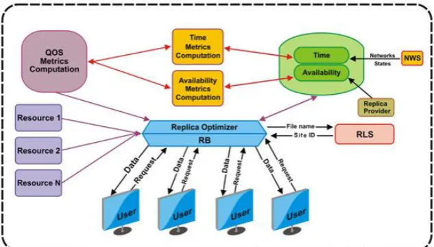
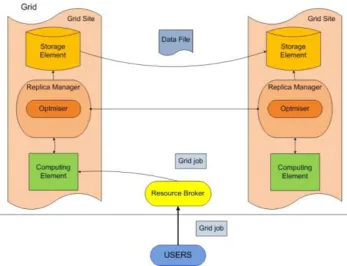
The architecture of the data grid services is divided into two levels as shown in Figure 1 [1]. The upper level includes the high-level services that utilize the low-level or core services. Replica selection optimization technique is high-level service so it invokes a number of core services. Information about an individual resource or set of resources is collected and maintained by a Grid Resource Information Service (GRIS) daemon [27]. GRIS is designed to gather and announce system configuration metadata describing that storage system. For example each storage resource in the Globus data grid [1] incorporates a GRIS to circulate its information. Typically, GRIS informs about attributes like storage capacity, seek times, and description of site-specific policies governing storage system usage. Some attributes are dynamic varying with various frequencies such as total space, the available space, queue waiting time and mount point. Others are static such as disk Transfer Rate.
Fig. 1. Major components and structure of data grid architecture. (Adopted from[1])
Weather Service (NWS)2 [28], Meta-computing Directory Service (MDS) [29] and Grid File Transfer Protocol (GridFTP) [29]. Then, the best replica site for the concerned user's job is chosen. In this context, the replica that promises the minimum response time with the least probability of disruption is the best. Hence, the new high-level service replica selection algorithm is an optimization approach. The proposed algorithm is designed to perform caching not replication. Caching [30] occurs on the user side; the user decides which replica is the best and copies the required replica to the local site. On the other hand, replication occurs on the server side; the server that houses the replicas decides which replicas are to be created and where to place them.
The exact sequence of steps in the proposed algorithm is as follows:
Collects jobs from the Resource Broker.
Collects replica of physical file names and locations from Replica Location Service.
Collects sites’ operating hours from their log files.
Collects sites’ current criteria values like bandwidth from the information service providers for instance GridFTP, NWS, and MDS.
Calculates the response time and site availability of each site and rates them by percentage. The site that demonstrates the best Response Time (T) will be given the value of 100% and the rest of sites will be rated based on their performance in comparison to the site that gets 100%. On the other hand, the rank of site availability100% will be given to the site or the sites that show sufficient time to complete the transfer even if the dynamic conditions of the network are degraded to some extent. A site is assigned 100% site availability if it shows availability equal to the predicted download time pulse the reserve time required to accommodate any decline in the network. Site availability of the remaining sites is rated based on the predicted download time and how much time is required for the reserve time.
Selects the best location that houses the required replica for the grid user. The best location is the one that shows minimum transfer time and the least probability of failure to complete the job due to site downtime.
This study focuses on incorporation of site availability as an essential element in the process of locating the best replica. Site availability in this work is defined as the relationship between the required time to download a replica and the remaining time declared by the site that offers this service. The remaining time of any site is the remaining over time to serve the user. The response time is defined as the time elapsed when moving data file from one site to another. The following subsections detail the calculation of site availability, response time, remaining time and the best site selection:
Data Grid Environment
Fig. 2. An overview of the new proposed algorithm
3.1. Calculating Time
Response time is a dynamic value changing as time passes based on the load on the network or the storage devices. However it is anticipated to be steady for a while or change slightly positively or negatively. But since it is difficult to estimate the response time in a dynamic manner, the response time can be estimated at the decision time (NWS applies fast statistical models to probe histories to make performance forecasts). The response time’s dynamicity is considered by integrating the new factor site availability (more details about site availability is in subsection B). The response time for a given site i is estimated by using the following equations proposed in a recently published work [31]:
Ti = T1i + T2i + T3i. (1)
T1 represents the transfer time, T2 represents the storage access latency and T3 represents the requested waiting time in the queue. T1 represents the data transmission via a wide area network, which depends on the network bandwidth, either a wide area network (WAN) or a local area network (LAN) and the file size which is computed by the following equation [32]:
. ) / (
(MB) 1 Bandwidth MB SEC
FileSize
In general, the operating systems schedule the disk I/O requests in a manner that improves system performance [33]. The process of scheduling is implemented by maintaining a queue of requests for the storage device. Therefore, the storage speed and the number of requests in the queue play a major role in the average response time experienced by applications. As a result, storage access latency (T2) is the delayed time of the storage machines to cater the requests and the delayed time depending on the file size and the storage type. Hence, T2 increased due to larger data files. Moreover, different storage machines have discrepant speeds (data transfer rates) during I/O operations. For example, a tape drive is slower than a disk pool and there are many types of tape drives with different speeds. For instance: the Hewlett-Packard (HP) Storage Works Ultrium 920 Drive speed = 120 MegaBytes per second (MBps) while the HP Storage Works Ultrium 448 Drive speed = 24 MBps [31]. Storage access latency (T2i) is calculated using the following equation:
. (MB/SEC) Speed
Storage
(MB) Size 2
File
T
i (3)Storage machines receive many requests at the same time, but they can only serve one request at a time. This leads to pending the requests on waiting in the queue. Input data transfer must be performed prior to an actual request. Similarly, output data transfer must be completed after an actual write process request. This buffering technique balances required time for requests waiting in the queue and the required time for storage media to serve the request in process [33]. Furthermore, the site will be busy during the period that it transfers any replica from the storage machine to the network. Any new incoming data requests have to wait for the transaction to complete and for the requests that join the queue prior to the underlying request [32]. Consequently, the new request should wait all the earlier requests to be processed in the storage queue. The waiting time is the sum of time from the first request in queue to the last. Each of these times is the storage access latency time T2. The request waiting time in queue (T3i) is calculated using the following equation:
n
i i
i
T
T
1. 2
3 . (4)
Data Grid Environment . Speed Storage Size BW Size 1 2
n i i iT
T
File File (5)However, it is worth mentioning that modern storage systems with disks and flash memories allow networking and storage to occur simultaneously. Hence, Equation 5 is modified as follows:
. Speed Storage Size BW Size MAX 1 2
n i i iT
T
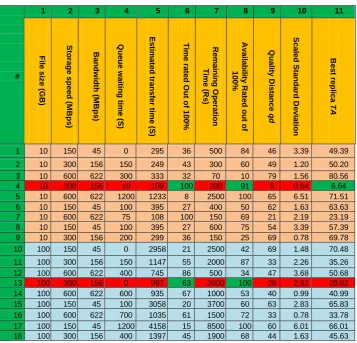
File File (5a)Table 1. 10 GB and 100 GB replicas with different metric values for: common
storage speed and bandwidth, queue waiting time and remaining time
#
1 2 3 4 5 6 7 8 9 10 11
F ile s iz e (G B ) Sto ra g e s p e e d (M B p s ) B a n d w id th (M B p s ) Q u e u e w a iti n g ti m e (S) Es ti m a te d tr a n s fe r ti m e (S) T im e r a te d O u t o f 1 0 0 % R e m a in in g O p e ra ti o n T im e (R s ) A v a ila b ili ty R a te d o u t o f 100% Q u a lity D is ta n c e qd Sc a le d Sta n d a rd D e v ia ti o n B e s t re p lic a TA
1 10 150 45 0 295 36 500 84 46 3.39 49.39
2 10 300 156 150 249 43 300 60 49 1.20 50.20
3 10 600 622 300 333 32 70 10 79 1.56 80.56
4 10 300 156 10 109 100 200 91 6 0.64 6.64
5 10 600 622 1200 1233 8 2500 100 65 6.51 71.51
6 10 150 45 100 395 27 400 50 62 1.63 63.63
7 10 600 622 75 108 100 150 69 21 2.19 23.19
8 10 150 45 100 395 27 600 75 54 3.39 57.39
9 10 300 156 200 299 36 150 25 69 0.78 69.78 10 100 150 45 0 2958 21 2500 42 69 1.48 70.48
11 100 300 156 150 1147 55 2000 87 33 2.26 35.26 12 100 600 622 400 745 86 500 34 47 3.68 50.68 13 100 300 156 0 997 63 2000 100 26 2.62 28.62 14 100 600 622 600 935 67 1000 53 40 0.99 40.99 15 100 150 45 100 3058 20 3700 60 63 2.83 65.83 16 100 600 622 700 1035 61 1500 72 33 0.78 33.78 17 100 150 45 1200 4158 15 8500 100 60 6.01 66.01 18 100 300 156 400 1397 45 1900 68 44 1.63 45.63
abovementioned data transfer speed models; any other valid model could easily replace the above mentioned models as an alternative solution.
Rating sites based on their response time (T0i) is denoted by the following equation:
. 100 min
{
1
0
T
T
i i n
i i
T
(6) For example, as shown in Table 1 which reflects real bandwidth, storage speeds and file sizes, the estimated download time based on Equation 5 from sites 1, 2, 3 and 4 are 295s, 249s, 333s and 109s respectively. Site 4 displays the minimum download time so it is rated as a 100% site, site 2 is ratedbased on Equation 6, 100 36%
295 109
while site 3 is rated
% 43 100 249 109
and site 3 is rated 100 32% 333
109
. As a result, all sites are
rated based on estimated download time to make the selection decision in the next step feasible and easier. The content of Table 1 will be discussed in detail in the following subsections.
3.2. Calculating Site Availability
Site availability is the relationship between the operating time declared by the service provider to serve certain VOs and the time required to transfer a file from the same provider during the replica selection process. Therefore, site availability (A) is computed as follows:
1. Ascertaining the remaining operation time (or allowed time) in seconds (Rs) from the site.
2. Estimating the required time to transfer the file (Ts). 3. Site availability is calculated by:
.
2 (SEC) Ts
(SEC)
Rs
A (7)
Data Grid Environment download time estimation is 100% accurate; the value of α is obtained from the history information by comparing the estimated transfer times with the actual transfer times. On the other hand, the maximum value of A should not exceed 100% because it is adequate and more than 100% is considered overqualified, which adds no values as demonstrated in Equation 8. In the example below, we assigned the value 1 to α, assuming 100% accuracy in download time estimation. However, based on our approach this number should be multiplied by 2 in order to be more confident that the transfer will commence and terminate from the same site and to avoid any risk of disconnection prior to download completion as shown in Equation 7. Hence, the minimum acceptable value for A is 50% but a higher value increases the success rate. On the other hand, estimating α requires more attention, which is outside the scope of this study. We plan to address this estimation issue in future work.
Site availability is rated as follows:
. Ts Rs , 100 2 (SEC) Ts
(SEC)
TS Rs , 100
0
Rs
A
(8)For example, using the same data shown in Table 1, the estimated download time based on Equation 5 from sites 1, 2, 3 and 4 are 295s, 249s, 333s and 109s respectively and the remaining operating time for each are 500s, 300s, 70s and 200s respectively. Assuming the value of α is 1, the site
availability for site 1 is 100 843% 1
2 295
500
, and the site availability for
site 2 is 100 60%
1 2 249
300
. The rest of the calculations are shown in Table
1.
3.3. Estimating the Best Site
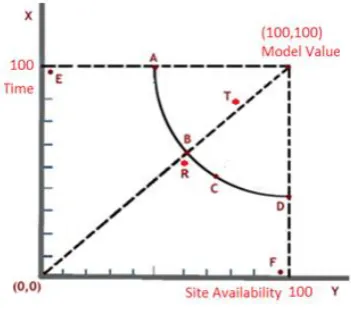
The new approach proposes an imaginary ideal or model value to be 100% Time (T) and 100% Site availability (A) as shown in Figure 3. The best site is the one with the closest distance (d) to the ideal value (T in Figure 3). We titled it as the quality distance (qd) which is calculated using the following equation:
2
0
100
2
0
100
T
2
A
qd
The distance in Equation 9 is divided by 2 to normalize its value to be between 0 and 100. The smaller the qd value, thebetter the site.
Fig. 3. Visual representation for sites and their model values
As shown in Figure 3, site T is the best site because it is the closest to the model value. If we do not have site T, the algorithm will select site A, B, C or D randomly because they all have the same distance from the Model value. In fact, the best in this scenario is site B because it is composed of two similar or almost similar values. This signifies a balanced solution, which is not extreme for site availability or transfer speed as opposed to site F. Site F displays high site availability but low quality transfer speed, which is still better than site A. Site A, displays high-quality transfer speed and low-quality site availability which could lead to a fault (disconnection). Moreover, it is clear that site R is better than sites A, C and D. To select a balanced solution and to avoid the extreme values as experienced in sites A or D as illustrated in Figure 3, the standard deviation (sd) is conceptualized by yielding a balanced optimal composition of time and availability. For example sd (70,70) = 0, sd (50,50) = 0, sd (30,30) = 0 while sd (60,40) = 14.14 and sd (70,30) = 28.28, and thus, the new equation for finding qd is modified to be as follows:
T
0A
0
sd
T
0A
0
2sd
100
0
2
0
100
2
qd
T
A
mqd (10)
Data Grid Environment Conversely, our experiments proved that adopting the standard deviation sometimes has side effects that could divert from the optimal solution. For example, if site X has the combination (63,100) for time and availability, utilizing Equation 10, mqd = 52.16 and site Y has the combination (61, 72), mqd = 40.78 meaning Y is better than X, even when it is clear that X is better than Y for both parameters, site availability and time. This example proves that the standard deviation has side effects and needs to be utilized wisely. To overcome the problem of standard deviation, it has been scaled down by dividing it into a number as in Equation 11. The result, site X rating is corrected to be better than Y. The other sites’ rates were corrected as well to reflect reality. The last version of mqd equation is denoted by:
A
T
0 0 sd2
0
100
2
0
100
2
T
A
mqd (11)
Estimating the value was carried out using a comprehensive search for all possible paired values of availability A and time T (A, T). We created a table containing all the possible values of A and T. The value 50 was assigned to availability in the first column, which is the minimum applicable value when =1, the second 51 and so on until the last column was given the value 100. We assigned the first row the value 30 for T and the second 31 until the last row was assigned the value 100. Table 2 depicts a summary of the real table. The objective is to find a value for that satisfies the following conditions:
1- Decreases the value of mqd (smaller mqd, better performance) while moving in the table from top to bottom. It is logical that the pair (50, 95) is better than (50, 30); certainly if we have both options we will choose the former.
2- Decreases the value of mqd while moving from left to right because it is logical that the pair (90, 30) is better than (50, 30).
3- Balances, to some extent, the values of A and T, for example (50, 50) is better than (90, 30) but (60, 44) is the best because 44 is faster than 30 and 60 is safer than 50.
Table 2. All possible paired values of availability A and time T and various values for
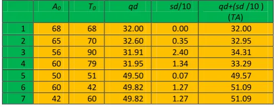
The modified distance mqd will be titled as TA in this study because it is composed of time and site availability and is given a new metric TA instead of meter (cm or km) because we are not measuring a normal distance. TA is derived from Time and Site availability where the site with the smallest TA is the best, since it is the closest to the imaginary ideal value. Table 3 is a mathematical example of our approach where column 1 represents the value of site availability; column 2, the estimated download time; column 3, the distance from the model value; column 4, the standard deviation of the two values for each site (estimated download time and site availability) divided by 10 and column 5, the total of columns 3 and 4. Again, as shown in Table 3, qd is the lowest in row 3, with the values 56, 90 TA for site availability and time respectively. However, it is clear that a value of 56 for site availability is very dangerous and thus prone to fault. As a result, this is not the best combination, even when the value of time is the highest. Therefore, standard deviation corrects the selection as can be seen in row 1, which shows the values site availability and time values of 68 each, as the best selection and row 2, as the second choice if row 1 is not available. On the other hand, the new algorithm excludes from the selection any site with site availability less than 50. For instance, referring to Table 3, if sites 1 to 5 do not exist and the competition is only between sites 6 and 7, and both of them have the same TA value, the winner is site 6 because the site availability for site 7 is less Than 50% which is for sure not enough.
Table 3, Example of applying the proposed algorithm
A0 T0 qd sd/10 qd+(sd /10 )
Data Grid Environment The pseudo code below emphasizes the detailed algorithm:
1. get R ( list of physical file names and locations for
the required replica) from RLS
2. get Rs for each replica from the data grid’s log file 3. estimate β
4. i=1
5. while R not empty 5.1 calculate T0, A0
5.2 calculate
A0
T0 sd 2
0 100
2 0
100 2 (i)
T A
mqd
5.3 i = i+1 6. best =
7. j=2
8. While j <= i
8.1 if < best & A0 > 50
8.1.1 best = 9. halt
4.
Performance Evaluation
Fig. 4. OptorSim architecture
5.
Simulation Setup
Data Grid Environment storing them locally with a storage capacity of 100 GB each and other sites which have at least one CE and a storage capacity of 50 GB each. The order in which a job requests files is determined by the Access Pattern used. Some different access patterns have been selected for the simulation. Such as sequential (all files are requested in a predetermined order), Gaussian random walk [37] (successive files are selected from a Gaussian distribution centered on the previous file) and Zipf. A Zipf-like distribution can be regarded as a special kind of exponential distribution allowing the simulation of several types of grid job. Additional essential feature is background network traffic, which can fluctuate variably over time. Any replica selection algorithm has to be flexible enough as to adapt to the constantly fluctuating environment, obtaining the best performance for its users.
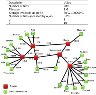
The default settings of OptorSim were utilized. They were copied from the EU data grid parameters. The bandwidth between the two sites is marked in Figure 5. In addition, the default OptorSim system workloads’ values and parameters’ values were utilized as shown in Table 4 (The detailed parameters’ values of each site are included in the example folder within OptorSim package. These values represent the real values of the EU data grid).
There are several configuration files used to control various inputs to OptorSim. The grid configuration file describes the grid topology and the content of each site. That is the resources available and the network connections to other sites. The job configuration file contains information on the simulated files, jobs and the site policies for each site (the list of files each site will accept). The simulation parameters file contains various simulation parameters which the user can modify. If the user wishes to simulate background network traffic, a bandwidth configuration file is needed along with several data files to describe the simulated traffic. The simulation accomplished on an Hp desktop with 2.8 G CPU and 2 G RAM. Since OptorSim does not consider site availability, it was amended by assigning service hours to each site ranged from 1second to 24 hours (sites available for less than 1 second are not declared by replica catalog). Thereafter, if the simulator faces a selected replica from a site with insufficient operating time, it will then increase the replica transfer time based on the expected delay. This is done by adding the reconnection setup time (10s) and half of the time consumed to transfer the replica before disconnection because fault tolerance techniques may require resuming or restarting from the beginning. In the simulation the average fault cost is calculated as follow:
Fault Cost = Rr+Trls+Rd+Cs+Ror (12)
Rr: Required time to recognize that there is a fault Trls: Time to inquire and get the response from RLS Rd: Replica selection decision time
Cs: Connection setup time
In the simulation, Rr and Trls are set to 2s each, Rd 1s and Cs set to 5s each. The total is 10s, which is not that critical for usually huge replicas but in contrast, Ror has a significant impact especially if the fault tolerance technique requires restarting from scratch. Fault tolerance techniques have an important impact to the replica selection process, which will be addressed in our future work.
Table 4, Workload and system parameter values
Description Value
Number of files File size
Storage available at an SE Number of files accessed by a job α
β
200 1 G
30 G-100000 G 3-20
1 10
Fig. 5. Grid topology for CMS test bed
6.
Performance Metrics & Cost
Data Grid Environment data files; the optimizer locates the best locations of the required files. However, each site services the users based on their local policy, which allows the users to be served for a specific number of hours per day or night, or even possibly, only on weekends. Hence, selecting the site at an improper time could lead to disconnection. Depending on the fault tolerance approach, the job could be resumed by another site (which may also be prone to disconnection if site availability is not considered or it may be required to restart the entire process from scratch. Therefore, the job’s time requirement will increase. The job’s time requirement begins from the time the RB transmits the job until the time that the job has completed its execution. This time is called the job turnaround time and includes the response time. The best replica selection according to the new algorithm decreases the response time and consequently decreases the job turnaround time. Therefore, the Average Job Turnaround Time (AJTT) is suitable for a performance metric that evaluates our overall algorithm performance and can be measured by using the following equation:
n AJTT
T
T
inn
i
out
1(13)
7.
Results and Discussion
OptorSim is equipped with different built-in replication strategies (i.e., Least Recently Used (LRU), which always replicates and deletes the least recently used file, Least Frequently Used (LFU), which always replicates and deletes the least frequently used file and the Economic Model-Binomial (EB), which replicates, if it is economically advantageous, using a binomial prediction function for values). However, within these replication strategies only one built-in replica selection algorithm is applied. It selects the best replica locations that show the least transfer time [30-31].
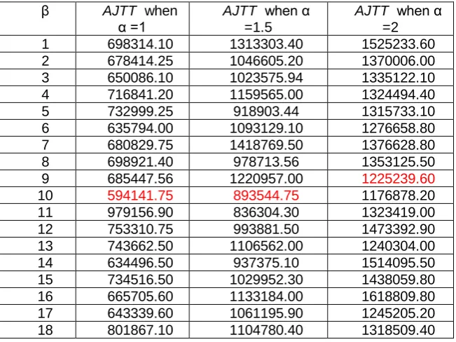
The simulations have been performed to calculate AJTT as the average of the total time required for all jobs, measured in seconds. The simulation commenced by investigating the best value for β. Several values were tested for β starting from 1 until 18. On the other hand, due to the fact that there is a strong relationship between α and β, the abovementioned tests were performed utilizing different values for α under LFU replication strategy. Table 5 depicts the results of these experiments wherein the best value of β is 10 when α =1 or 1.5, and the best value of β is 9 when α =2.
Table5, Average jobs’ time in seconds for 500 jobs with different values of α and β
β AJTT when
α =1 AJTT=1.5 when α
AJTT when α =2
1 698314.10 1313303.40 1525233.60
2 678414.25 1046605.20 1370006.00
3 650086.10 1023575.94 1335122.10
4 716841.20 1159565.00 1324494.40
5 732999.25 918903.44 1315733.10
6 635794.00 1093129.10 1276658.80
7 680829.75 1418769.50 1376628.80
8 698921.40 978713.56 1353125.50
9 685447.56 1220957.00 1225239.60
10 594141.75 893544.75 1176878.20
11 979156.90 836304.30 1323419.00
12 753310.75 993881.50 1473392.90
13 743662.50 1106562.00 1240304.00
14 634496.50 937375.10 1514095.50
15 734516.50 1029952.30 1438059.80
16 665705.60 1133184.00 1618809.80
17 643339.60 1061195.90 1245205.20
18 801867.10 1104780.40 1318509.40
Data Grid Environment which reflects better performance. Because the scope of this study is only site availability, and it is anticipated that grid systems are still using legacy storage systems, the remaining experiments were carried out based on Equation 5.
Table6. Average jobs’ times in seconds for 500 jobs based on Equations 5 and 5a
Table 7. Average jobs’ times in seconds for 100 jobs when availability is always
100%
To verify that the only difference between the proposed algorithm and the built-in in OptorSim is site availability, both algorithms were run with site availability always set to 100%. The expectation was that similar performance would be achieved from both because response time is the only selection factor in the built-in OptorSim and should be in the proposed algorithm when site availability is 100%. However, the simulation results in Table 7 below were surprising. They show that the proposed algorithm is less efficient in all
Test # LUR LFU Economic
Eq 5a Eq 5 Eq 5a Eq 5 Eq 5a Eq 5
1 12756230 11839082 8973130 11083612 8856054 8628327 2 9173741 8574796 11902111 12664846 9315399 9670981 3 9474930 9842670 10641312 10206533 8758650 9393326 4 8839858 12177088 8817204 12174020 7927166 10171052 5 10249128 10639864 9871939 11989452 9487867 10921624
AJTT 10098777 10614700 10041139 11623692 8869027 9757062
Ef fici en c y ba sed on Eq
5a 4.86% 13.61% 9.10%
Te
st
#
LUR LFU Economic
P ro p o se d A lgo ri th m O p to rS im B u ilt -in A lgo ri th m P ro p o se d A lgo ri th m O p to rS im B u ilt -in A lgo ri th m P ro p o se d A lgo ri th m O p to rS im B u ilt -in A lgo ri th m
1 286111 231099 278278 230458 1060176 906395 2 275035 242358 271168 220449 1085247 1035999 3 284864 222627 255691 223970 913550 904781 4 238518 232944 288959 216565 1005183 954523 5 256388 224360 242888 224768 977966 1062441
AJTT 268183 230678 267397 223242 1008424 972828
Ef fici en cy of the pr opos ed A lgor
three of the replication strategies. The justification for that is the number of jobs in this experiment is 100. Each of them is accompanied by 10 to 100 replicas, which means on average around 5500 replicas (decisions). Therefore, there will certainly be some overhead.
Table 8 (a). Average jobs’ times in seconds for 100 jobs
Based on the abovementioned experiments, the remaining simulation experiments were carried out by setting the value of β to 10. In view of the fact that the number of jobs influenced data transfer time, we evaluated our algorithm’s performance in three different scenarios by varying the number of jobs each time. In the first, second and third scenarios, the number of jobs were 100, 500 and 1000 respectively.
We executed the simulation 5 times for each scenario along with a predetermined site operating time scenario, utilizing both our algorithm and the built-in extended algorithm in OptorSim. We did our experiments using three different OptorSim built-in replication strategies, namely, LRU, LFU and EB. Our new replica selection algorithm was tested by performing several executions on the same replicas with a different number of jobs. The results of the simulation demonstrated that the AJTT in the new algorithm was less than the AJTT of the OptorSim built-in replica selection algorithm for all scenarios and under different replication strategies as shown in Tables 8 (a, b, c), which signified that the proposed algorithm outperformed the previous algorithms.
Te
st
#
LUR LFU Economic
P ro p o se d A lgo ri th m O p to rS im B u ilt -in A lgo ri th m P ro p o se d A lgo ri th m Op to rS im B u ilt -in A lgo ri th m P ro p o se d A lgo ri th m O p to rS im B u ilt -in A lgo ri th m
1 704189 1278467 628694 1544662 933333 932571 2 582321 1090155 747886 1013950 909764 855317 3 582266 1280359 579806 1243939 836163 946263 4 720064 1105045 706270 1248695 855435 956849 5 650280 1041018 648674 1161950 934881 964598
AJTT 647824 1159009 662266 1242639 893915 931120
Ef fici en cy of the pr opos ed A lgor
Data Grid Environment
Table8(b). Average jobs’ times in seconds for 500 jobs
Table8 (c). Average jobs’ times in seconds for 1000 jobs
Figure 6 (a, b, c) depicts the average jobs’ total time for the proposed algorithm and the OptorSim built-in algorithm under the replication strategies LRU, LFU and EB where the number of jobs was 100, 500 and 1000 respectively. It is clear that when we increase the number of jobs AJTT will be increased regardless of the algorithm or the strategy utilized. However, the increment will be more if site availability is not implemented in the algorithm; this is because the probability of selecting unavailable sites, or sites available for an insufficient amount of time, increases.
Te
st
#
LUR LFU Economic
P ro p o se d A lgo ri th m O p to rS im B u ilt -in A lgo ri th m P ro p o se d A lgo ri th m O p to rS im B u ilt -in A lgo ri th m P ro p o se d A lgo ri th m O p to rS im B u ilt -in A lgo ri th m
1 12108976 17167802 9644758 19077332 9065388 8516753 2 11204400 15578618 11485171 12449995 9751129 8698534 3 8571915 17896652 9990595 17365892 8654000 9336498 4 12741477 14618266 11045485 16848332 8335365 10864292 5 9886645 14733334 10801072 13096076 9451450 9190288
AJTT 10902682 15998934 10593416 15767525 9051466 9321273
Ef fici en cy of the pr opos ed A lgor
ithm 31.85% 32.81% 2.89%
Te
st
#
LUR LFU Economic
P ro p o se d A lgo ri th m O p to rS im B u ilt -in A lgo ri th m P ro p o se d A lgo ri th m O p to rS im B u ilt -in A lgo ri th m P ro p o se d A lgo ri th m O p to rS im B u ilt -in A lgo ri th m
1 44425416 59635972 41978100 51684568 30145046 291046946 2 41558504 72720032 44334344 73405680 24623898 24063774 3 41331136 64606356 41013108 67973424 26333746 27421194 4 45374036 60879928 42693512 58488172 28583260 26592294 5 45420436 83777552 42533128 75843184 28765640 26274540
AJTT 43621905 68323968 42510438 65479005 27690318 79079749
Ef fici en cy of the pr o pos ed A lgor
Fig. 6 (a). Average jobs’ total time in seconds for 100 jobs
Data Grid Environment
Fig. 6 (c). Average jobs’ total time in seconds for 1000 jobs
In real life scenarios, replica selection based only on response time could perform better than the proposed algorithm if the selected sites display insufficient availability but still succeed to deliver the replicas without any disconnection, or if all the sites are available 24 hours per day
8.
Conclusion
References
1. S. Vazhkudai, S. Tuecke, and I. Foster, "Replica selection in the globus data grid," in Cluster Computing and the Grid, Brisbane, Qld. , Australia 2001, pp. 106-113.
2. A. Chervenak, E. Deelman, I. Foster, L. Guy, W. Hoschek, A. Iamnitchi, C. Kesselman, P. Kunszt, M. Ripeanu, and B. Schwartzkopf, "Giggle: a framework for constructing scalable replica location services," in 2002 ACM/IEEE conference on Supercomputing, Baltimore, Maryland 2002, pp. 1-17.
3 C. Dumitrescu and I. Foster, "GRUBER: A Grid resource usage SLA broker," Euro-Par 2005 Parallel Processing, pp. 644-644, 2005.
4. M. Lei, S. V. Vrbsky, and X. Hong, "An on-line replication strategy to increase availability in Data Grids," Future Generation Computer Systems, vol. 24, pp. 85-98, 2008.
5. D. Zeinalipour-Yazti and N. Kyriacos, "Managing Failures in a Grid System using FailRank," Department of Computer Science,University of Cyprus2006.
6. I. Foster, J. Gieraltowski, S. Gose, N. Maltsev, E. May, A. Rodriguez, D. Sulakhe, A. Vaniachine, J. Shank, and S. Youssef, "The Grid2003 production Grid: Principles and practice," in 13th IEEE International Symposium on High performance Distributed Computing, 2004, Honolulu, Hawaii, 2004, pp. 236-245. 7. (2011, 6-11). Open Science Grid Consortium. Available:
http://www.opensciencegrid.org
8. (2011, 28/10). LCG Grid. Available: http://www.gridpp.ac.uk.
9. M. Aggarwal, D. Colling, B. McEvoy, G. Moont, and O. Aa v. d., "A Statistical Analysis of Job Performance within LCG Grid," presented at the CHEP06, Mumbai, India, 2006.
10. S. Lewontin and E. Martin, "Client side load balancing for the web," in 6th International World Wide Web Conference, Santa Clara, California, 1997, pp. 7-11.
11. Z. M. Fei, S. Bhattacharjee, E. W. Zegura, and M. H. Ammar, "A novel server selection technique for improving the response time of a replicated service," in Seventeenth Annual Joint Conference of the IEEE Computer and Communications Societies., San Francisco, CA , USA 1998, pp. 783-791 vol. 2. 12. L. Zuo, S. H. Liu, J. Wei, Y. L. Feng, and G. C. Fan, "Adaptive component replica
selection model and algorithms," Ruan Jian Xue Bao(Journal of Software), vol. 19, pp. 1212-1223, 2008.
13. R. Vingralek, Y. Breitbart, M. Sayal, and P. Scheuermann, "Web++: A system for fast and reliable web service," in USENIX Annual Technical Conference, USA, 1999, pp. 13-13.
14. M. Sayal, Y. Breitbart, P. Scheuermann, and R. Vingralek, "Selection algorithms for replicated web servers," ACM SIGMETRICS Performance Evaluation Review, vol. 26, pp. 44-50, 1998.
15. C. Tan and K. Mills, "Performance characterization of decentralized algorithms for replica selection in distributed object systems," in the 5th international workshop on Software and performance, New York, NY, USA 2005, pp. 257-262. 16 R. Kavitha and I. Foster, "Design and evaluation of replication strategies for a
high performance data grid," in International Conference on Computing in High Energy and Nuclear Physics, Beijing, China 2001.
Data Grid Environment 18. S. Vazhkudai and J. M. Schopf, "Using regression techniques to predict large data transfers," International Journal of High Performance Computing Applications, vol. 17, p. 249, 2003.
19. R. M. Rahman, R. Alhajj, and K. Barker, "Replica selection strategies in data grid," Journal of Parallel and Distributed Computing, vol. 68, pp. 1561-1574, 2008.
20. C. ze Wu, K. gui Wu, M. Chen, and C. X. Ye, "Dynamic Replica selection services based on state evaluation strategy," in Fourth ChinaGrid Annual Conference, 2009, Yantai, Shandong 2009, pp. 116-119.
21. J. Feng and M. Humphrey, "Eliminating replica selection-using multiple replicas to accelerate data transfer on grids," 2004, pp. 356-366.
22. K. C. Li, H. H. Wang, K. Y. Cheng, and T. Y. Wu, "Strategies Toward Optimal Access to File Replicas in Data Grid Environments," Journal of Information Science and Engineering, vol. 25, pp. 747-762, 2009.
23. V. Vijayakumar and R. S. D. W. Banu, "Security for resource selection in grid computing based on trust and reputation responsiveness," International Journal of Computer Science and Network Security, vol. 8, pp. 107-115, 2008.
24. G. Kavitha and V. Sankaranarayanan, "Secure Resource Selection in Computational Grid Based on Quantitative Execution Trust," World Academy of Science, Engineering and Technology, vol. 72, pp. 149-155, 2010.
25. B. Zhang, Y. Xiang, and Q. Xu, "Trust and Reputation Based Model Selection Mechanism for Decision-Making," in Second International Conference on Networks Security Wireless Communications and Trusted Computing, 2010, Wuhan, Hubei 2010, pp. 14-17.
26. S. Naseera, T. Vivekanandan, and K. Madhu Murthy, "Data Replication Using Experience Based Trust in a Data Grid Environment," Distributed Computing and Internet Technology, vol. 1, pp. 39-50, 2009.
27. D. H. Kim and K. W. Kang, "Design and implementation of integrated information system for monitoring resources in grid computing," in 10th International Conference on Computer Supported Cooperative Work in Design Nanjing, 2006, pp. 1-6.
28. R. Wolski, "Dynamically forecasting network performance using the network weather service," Cluster Computing, vol. 1, pp. 119-132, 1998.
29. S. Fitzgerald, I. Foster, C. Kesselman, G. Von Laszewski, W. Smith, and S. Tuecke, "A directory service for configuring high-performance distributed computations," 1997, pp. 365-375.
30. K. Ranganathan and I. Foster, "Identifying dynamic replication strategies for a high-performance data grid," Grid Computing—GRID 2001, pp. 75-86, 2001. 31. H. H. E. AL-Mistarihi and C. H. Yong, "Response Time Optimization for Replica
Selection Service in Data Grids," Journal of Computer Science, vol. 4, pp. 487-493, 2008.
32. K. Ranganathan and I. Foster, "Identifying dynamic replication strategies for a high-performance data grid," in the Second International Workshop on Grid Computing Denver,CO,2001, 2001, pp. 75-86.
33. S. Aberham, P. Baer, and G. Greg, Operating System Concepts Seventh ed. vol. 5. New York, NY, USA.: Wiley, 1973.
34. S. M. Ross, Introduction to probability models, 6th ed.: Academic Pr, 1997. 35. A. Sulistio, C. S. Yeo, and R. Buyya, "A taxonomy of computer‐based
36. W. H. Bell, D. G. Cameron, R. Carvajal-Schiaffino, A. P. Millar, K. Stockinger, and F. Zini, "Evaluation of an economy-based file replication strategy for a data grid," in 3rd IEEE/ACM International Symposium on Cluster Computing and the Grid, 2003, Tokyo, Japan, 2003, pp. 661-668.
37. W. H. Bell, D. G. Cameron, A. P. Millar, L. Capozza, K. Stockinger, and F. Zini, "Optorsim: A grid simulator for studying dynamic data replication strategies," International Journal of High Performance Computing Applications, vol. 17, pp. 403-416, 2003.
Ayman Jaradat has obtained his MSc from Universiti Sains Malaysia in 2007 and BSc, Yarmouk University, Jordan in 1989. He is specialized in Computer Science more specifically in distributed systems. His research interest includes grid computing which focuses on data grids, genetic algorithm, distributed algorithms and applications. Jaradat is currently pursuing his PhD at Universiti Teknologi PETRONAS, Malaysia.
Ahmed Patel received his MSc. and PhD. degrees in Computer Science from Trinity College Dublin (TCD), Ireland. He is a Professor in Computer Science at Universiti Kebangsaan Malaysia. His research interests is in Cloud & Grid Computing, Smart Grid, Cyber Security & Digital Forensics. He has published well over 220 technical and scientific papers and co-authored 2 books on computer network security and 1 book on group communications, and co-edited a book distributed search systems for the Internet.
Nordin Zakaria has obtained his PhD from Universiti Sains Malaysia in 2007, MSc from Universiti Malaya in 1999, and BSc from Universiti Putra Malaysia in 1996. Zakaria is specialized in Computer Science and his research interest includes high-performance computing, genetic algorithm, distributed algorithms and applications. Zakaria was assigned to establish and lead the High-Performance Computing Service Center at Universiti Teknologi PETRONAS.
Anang Hudaya Muhamad Amin is a senior lecturer in the Department of Computer & Information Sciences, Universiti Teknologi PETRONAS (UTP), Malaysia. He received a BTech (Hons.) in Information Technology from UTP, Malaysia, and Master of Network Computing and PhD. from Monash University, Australia. His research interests include artificial intelligence with specialization in distributed pattern recognition and bio-inspired computational intelligence, wireless sensor networks and distributed computing.
![Fig. 1. Major components and structure of data grid architecture. (Adopted from[1])](https://thumb-us.123doks.com/thumbv2/123dok_us/1176968.1620348/5.595.140.458.416.580/fig-major-components-structure-data-grid-architecture-adopted.webp)