Using Part-of-Speech Tags as Deep-Syntax Indicators in
Determining Short-Text Semantic Similarity
Vuk Batanović1 and Dragan Bojić2
1 School of Electrical Engineering, Bulevar kralja Aleksandra 73,
11120 Belgrade, Serbia [email protected]
2 School of Electrical Engineering, Bulevar kralja Aleksandra 73,
11120 Belgrade, Serbia [email protected]
Abstract. This paper presents POST STSS, a method of determining short-text semantic similarity in which part-of-speech tags are used as indicators of the deeper syntactic information usually extracted by more advanced tools like parsers and semantic role labelers. Our model employs a part-of-speech weighting scheme and is based on a statistical bag-of-words approach. It does not require either hand-crafted knowledge bases or advanced syntactic tools, which makes it easily applicable to languages with limited natural language processing resources. By using a paraphrase recognition test, we demonstrate that our system achieves a higher accuracy than all existing statistical similarity algorithms and solutions of a more structural kind.
Keywords: short-text semantic similarity, statistical similarity, corpus-based measures, part-of-speech tags, POS weighting, syntactic information, bag-of-words model, natural language processing.
1.
Introduction
Determining the semantic similarity of short texts means assigning a certain metric to a given pair of texts based on the level of semantic matching between them. Semantic similarity systems provide a standard score between zero and one, where zero denotes complete semantic dissimilarity, and one full semantic equivalence. Short-text semantic similarity (STSS) is especially important since short texts are widely used on the Internet as search queries and results, comments on social networks, news headlines and snippets, product tags, etc.
from the one used in the document that contains the answer. Hence, taking those variations into account can lead to improvements in system performance [2].
There are two basic approaches to determining the semantic similarity of two words: the topological or knowledge-based one, which uses expert knowledge, and the
statistical or corpus-based one, which uses a text corpus. Topological similarity determines the semantic relatedness between words by using hand-crafted ontologies like WordNet [3]. Since such structures are created by using expert human knowledge, they are able to model the degrees of semantic relatedness between words quite successfully when suitable distance metrics are applied. However, significant human effort is required to create resources of this kind, rendering the topological approach inapplicable to many minor languages or languages with scarce NLP resources. A recent study [4] found that there are currently around 40 projects to build wordnets for various languages. Only about a third of them are available under a free, open-source license, while a further third are free solely for academic research. In comparison, there are over 7000 languages spoken in the world today [5], 1300 of which are spoken by more than 100,000 people. Moreover, many existing wordnet projects are still in inception, with a rather limited number of words and synsets included, making them unsuitable for complex NLP tasks like STSS.
On the other hand, the only resource required in the implementation of statistical methods is a text corpus, which makes them widely and easily applicable. Statistical approaches to semantic similarity rely on the distributional hypothesis, which states that words with similar meanings tend to appear in similar contexts [6]. By applying this hypothesis to a large text corpus, it is possible to create a semantic space in the shape of a co-occurrence matrix. In this matrix every word found in the corpus has its own row and every context its own column. Cells of the matrix specify how many times each word appeared in each context. A context can usually be either a document from the corpus, or another word in whose proximity the given word appeared. In this way each word is assigned a context vector, which makes it possible to compare word meanings by comparing their vectors.
A newer statistical viewpoint is based on the probabilistic approach to semantics, which originates in the field of topic modeling [7]. Topic models treat each document within a text corpus as a mixture of corpus-wide topics, and each topic as a distribution over a certain vocabulary. Topic modeling algorithms use the textual documents to infer the distribution of topics in the corpus, the document topic proportions, and the per-word topic assignments. Since per-words can occur in multiple topics with different probabilities, they can be viewed in terms of their topic contributions. By comparing those contributions it is possible to compare word meanings.
This paper is organized as follows: in Section 2 we give an overview of current STSS systems. Section 3 outlines the main ideas of our approach and the motivation behind it, and presents certain existing algorithms and tools used within it. In Section 4 we describe the corpus processing procedures which we employed. Section 5 contains a detailed explanation and an example of the operation of our proposed system and the way it utilizes POS tags. In Section 6 we elaborate on the procedure used to train and optimize our model. Section 7 presents an evaluation of our method and a comparison to other approaches. Finally, in Section 8 we summarize our work and point towards possible system improvements and directions for future research.
2.
Related Work
Numerous STSS solutions, both topological and statistical, already exist, and many of them use some form of syntactic information. In terms of their approach toward syntax, there are two main types of STSS systems:
1. Systems which ignore sentence structure by employing a bag-of-words technique. In this model, a sentence is treated as an unordered set of words, thereby ignoring the organization and interdependence of words within a sentence. These systems sometimes use shallow syntactic information, such as POS tags, but mostly in a superficial manner.
2. Systems which adopt a more structural approach to semantics by harnessing deep syntactic information. These systems use more advanced NLP tools like parsers and semantic role labelers.
In relation to STSS systems, there also exists an entire family of algorithms which deal with the issue of paraphrase identification, i.e. of determining whether sentences in a given pair are paraphrases of each other or not. Such algorithms commonly employ advanced machine learning classifiers and a wealth of features, oftentimes including syntactic ones, to arrive at a binary decision ([9], [10]). However, it should be pointed out that the task of generating a binary classification is a much more limited and easier one than the task of interval-based semantic gradation performed by STSS methods.
2.1. Bag-of-Words Models
weaker form of this restriction which relies only on basic word classes, e.g. verbs, and not on their subtypes like infinitives, past tenses, participles, etc.
Rus et al. [14] experimented with the same LSA algorithm alongside LDA (Latent Dirichlet Allocation), a topic modeling method, within a syntactically simpler approach in which no POS information is utilized. Quan et al. [15] devised another approach based on topic modeling, called TBS (Topic Based Similarity). It compares short texts on the basis of their common words, as well as the probabilities of their distinguishing terms under each probabilistic topic.
Ramage et al. [16] proposed a method that does not compare two bags-of-words directly but instead compares the distributions induced by each text when used as the seed of a random walk over a graph, which is constructed by using both WordNet and a text corpus. POS information is utilized during the graph construction phase, and as a part of text preprocessing, thus allowing the model to more accurately match the words in the given text with the nodes in the graph on which it operates.
Guo and Diab [17] also use POS tagging as a corpus preprocessing step within a latent semantic model of sentences called WTMF (Weighted Textual Matrix Factorization). Their method explicitly models the words that are not present in the sentences, but takes into account the fact that the missing words are not as informative as the observed ones.
The approach devised by Islam and Inkpen [18] does not employ POS tags but instead combines string similarity with corpus-based semantic similarity. They also experimented with the inclusion of a measure of the common-word order between the two given texts. Furlan et al. [19] modified their model to utilize the more advanced COALS (Correlated Occurrence Analogue to Lexical Semantic) statistical algorithm. Furlan et al. [20] further developed this method into a language-independent, corpus-based approach called LInSTSS which relies on term frequency weighting.
2.2. Structural Models
Structural solutions of the second kind include the one from Li et al. [21] which uses shallow parsing to divide each sentence into noun phrases (NP), verb phrases (VP), and preposition phrases (PP). Their method then compares the meanings of sentences by comparing the appropriate phrases within them, while individual word meanings are acquired through the use of WordNet. In addition, Li et al. experimented with a similar approach [22] in which sentences are compared based on the objects that appear in them, as well as the properties of those objects and their behavior. Shallow parsing is used to extract noun and verb phrases from each sentence. Their method groups the nouns from noun phrases as objects, the adjectives and adverbs from noun phrases as object properties, while verb phrases are grouped as object behaviors. The final similarity of sentences is determined as a sum of the similarities of these three groups, while the word-to-word similarities are calculated by using WordNet.
contains certain syntactic structures not present in the other. Like [11], [12], and [13], Oliva et al. also experimented with various WordNet metrics, and employed POS information in a similar way.
Lee et al. [24] considered a combination of string similarity metrics similar to the ones used in [18] and a syntactic pattern matching mechanism which identifies subject-verb-object structures in each sentence. This mechanism relies on the use of a parser, while the word-to-word semantic similarities are determined by using WordNet. Lee et al. [25] also proposed a different topological method that treats a sentence as a sequence of links, each of which contains a specific meaning and connects a pair of words. In order to extract such links it uses a syntactic parser called Link grammar.
Furlan et al. [19] described a knowledge-based algorithm that employs a semantic net called ConceptNet as the word data model. They use a semantic role labeling module to extract subject-verb-object tuples from each sentence. Achananuparp et al. [26] proposed a way to address the syntactic variability of language expression by measuring the similarity of sentences via verb-argument structures. Such structures are obtained through semantic role labeling and the final similarity score is calculated as a sum of the similarities of verbs, determined by using WordNet, and their corresponding arguments.
Several structural solutions employ a weighting scheme of some kind, in which the similarities of different constituents are given different weights. This is accomplished by weighting according to semantic roles ([19], [23]), phrase types [21], or a combination of phrase types and word types [22]. In some methods weighting is an optional component whose effects were not explored [24]. Other authors concluded that their methods perform best when equal weighting is utilized [26].
3.
Proposed Method
The central idea of our proposed method is that certain parts of speech and certain relationships between different parts of speech are semantically more important than others, not only inherently, but also due to the roles they commonly play within a sentence. By taking account of this notion, our STSS system is able to utilize POS tag information as an indicator of the deeper underlying syntactic structure.
3.1. Motivation
It is rather intuitive that not all elements of a sentence carry the same amount of semantic information. For instance, let us consider the following sentences:
1. I drank some coffee. 2. I drank some milk.
3. I bought some milk.
Hence, the use of weighting strategies in some of the existing STSS systems does have a sound justification. However, such a strategy has, so far as we know, never been implemented solely on the part-of-speech level. All existing STSS systems that employ weighting are structural ones. They use advanced syntactic tools – parsers and semantic role labelers – to delineate constituents by harnessing deeper syntactic information.
As far as the existing bag-of-words methods are concerned, almost all of them either do not utilize POS tags at all, or they do so rather superficially and usually in order to prevent the pairing of words belonging to different parts of speech. This usage, though logical at first glance, can in fact easily lead to errors. Let us consider, for example, the following sentence pair:
– He is a diligent worker.
– He works diligently.
Although these two sentences carry the same meaning, the combination of an adjective and a noun from the first sentence (diligent worker) is replaced by a combination of a verb and an adverb in the second (works diligently). In such cases, it would be a mistake to forbid the pairing of words (worker, works) and (diligent,
diligently), even though the words comprising those pairs belong to different parts of speech. Similar examples can be found in pairs of sentences where one sentence is in the active and the other in the passive voice:
– They finished constructing the bridge.
– The construction of the bridge was finished.
The words constructing and construction do not belong to the same part of speech, but it is clear that the pairing of those words is appropriate and should not be prohibited.
3.2. POST STSS
Our method, which we call POST STSS (POS-tag-supported STSS), combines a weighting strategy based on POS tags with a bag-of-words approach. Although POS tags offer only a shallow representation of sentence structure, we argue that through their use it is possible to obtain much of the information usually provided by the more complex, but also more error-prone NLP tools. In addition, we recognize the merits of allowing the coupling of certain parts of speech and disallowing the pairing of others, but we handle such rules much more carefully than did the previous STSS solutions.
utilized the algorithm implementation provided by the S-Space package [29], with the default setting of 14000 for the initial size of the co-occurrence matrix. Its dimensionality is then reduced to 800 through SVD.
For text preprocessing we used the Stanford CoreNLP package [30]. This suite encompasses many NLP tools, including a tokenizer, a sentence splitter, a lemmatizer, a POS tagger, a named entity recognizer, a dependency parser, and a coreference resolution tool. They are all tied together in a modular fashion, making it easy to take advantage of the more advanced functions, if needed. In our system we utilized only the tokenizer, the sentence splitter, the lemmatizer, and the POS tagger. The POS tagger is based on a log-linear approach and achieves an accuracy of over 97% [31].
4.
Corpus Processing
The text corpus chosen for the creation of the POST STSS system needed to be sufficiently large, topically diverse, and publicly available, which is why we selected the English Wikipedia abstract corpus. This corpus contains short text summaries of all the articles present in the English Wikipedia. Its size, at the time, was around 3.7 GB. Since the corpus is available as an XML file which, aside from the abstracts, also includes other irrelevant information, we had to scan through the file to extract the useful data. We then cleaned the text by eliminating all numbers and words that contain numbers, by removing all punctuation marks, and by normalizing all letters into lower case.
We tested two text preprocessing procedures on our system: stemming and lemmatization. Stemming is a transformation in which a given word is stripped of its suffixes, thereby reducing it to its stem. In this manner, multiple different words can be normalized into a single morphological form, thus reducing the overall number of different words. Hence, the application of stemming to a text corpus ultimately leads to the creation of a smaller semantic space. This can, in effect, reduce the overall computational costs. In our system we utilized the standard Porter stemmer [32].
Despite their advantages, stemmers also have their drawbacks, like their inability to cope with prefixes. However, the biggest issue concerning stemmers is their propensity to make mistakes. For instance, the words animal, animation, and animism, although semantically diverse, will all be reduced to a single stem – anim. While such errors are the exception rather than the rule, numerous other examples can be found. In a semantic space, these mistakes can trigger the merger of words which have completely unrelated meanings, consequently having a detrimental effect on system performance. These problems are further exacerbated when working with highly inflectional languages.
Still, unlike stemmers, which operate on individual words with no knowledge of the surrounding context, lemmatizers have to be able to discriminate between words that can have different meanings depending on their part of speech. Thus, a POS tagger is required for their operation. Since we devised our STSS model around using POS tags, it was simple to add lemmatization to it, via the appropriate Stanford CoreNLP module.
After stemming or lemmatizing our text corpus, we created the semantic space by supplying the processed corpus to the COALS algorithm. The produced semantic space was saved to the hard drive in the Sparse Text format, defined in the S-Space package.
5.
System Operation
The POST STSS approach employs the method proposed in [18] of matching each word in the shorter text P to its most similar counterpart in the longer text R, and then adding up the individual similarity scores, based on both the string and the semantic similarity, into a unified measure. We improve this method by weighting word similarity scores using values determined on the basis of both words’ POS tags.
Determining the semantic similarity of two short texts begins by creating annotation modules from the Stanford CoreNLP package for tokenizing, sentence splitting, part-of-speech tagging, and lemmatizing, and applying them to both texts. Properly identifying the placement of sentence boundaries in a given short text is important for the proper functioning of POS tagging. Words are tokenized, and POS tagging is subsequently performed. Tokens are then either stemmed or lemmatized. Finally, all tokens containing numbers or other non-alphabetic characters are excluded from further consideration, thus generating the processed texts and their POS tag sequences. The number of tokens in the shorter text P will hereafter be referred to as m, while the number of tokens in the longer text R will be n.
We then identify the words which appear in both texts, whose count we will refer to as d. Since those words are identical in both P and R, both their string and semantic similarities are maximal. Hence, their final similarity measures depend only on their POS tags. We describe the precise manner of POS weighting in Section 5.3. The scores of all of the words appearing in both texts are added up into a similarity sum Ssame.
The remaining m – d and n – d words from both texts are used to construct three (m – d) × (n – d) matrices in which the remaining words from the shorter text P are assigned to the rows of the matrix, whereas the columns of the matrix represent words from the longer text R. These matrices are:
1. The string similarity matrix; 2. The semantic similarity matrix; 3. The POS weighting matrix.
5.1. String Similarity
way as [18], we calculate this similarity score by combining the following three modifications of the LCS (Longest Common Subsequence) metric:
– NLCS – Normalized Longest Common Subsequence;
– NMCLCS1 – Normalized Maximal Consecutive Longest Common Subsequence starting at character 1;
– NMCLCSN – Normalized Maximal Consecutive Longest Common Subsequence starting at character N.
Unlike the LCS where consecutiveness is not required, the second and the third modification only search for the longest consecutive common subsequence. The second algorithm searches for the maximal consecutive portion of the shorter string that consecutively matches with the longer string, where matching starts from the first character in both strings. The third algorithm does the same, but allows the matching to start at any character in both strings. In all three modifications the basic similarity value is divided by the length of both strings compared, thereby normalizing the score. The final string similarity score is gained by summing the individual scores of these three metrics, while giving each an equal weight.
5.2. Semantic Similarity
In the semantic similarity matrix each cell has a value that represents the level of semantic similarity between the row-word and the column-word. We obtain this score by taking the context vectors of the two words being compared and calculating their cosine similarity. The context vectors are extracted from the semantic space generated by COALS. A score of zero indicates total semantic dissimilitude while a score of one signifies a complete semantic match. COALS can also produce negative similarity scores for certain vector pairs, as a side effect of the SVD operation, but this occurs relatively rarely [28]. As far as we have noticed, such scores tend to have low absolute values. We experimented with setting those scores to zero, but found no performance benefit from doing so and, hence, we ultimately retained them.
5.3. POS Weighting
Our POS weighting method uses a set of weights for different POS tags and a POS interaction matrix. The POS interaction matrix is a symmetric matrix which consists of binary values specifying for any two diverse tags whether the coupling of words that have those tags assigned to them should be allowed or not. In other words, the POS interaction matrix determines which diverse part-of-speech couplings are allowed and which are forbidden.
When comparing two words that belong to the same part of speech we simply place the weight for that part of speech in the appropriate cell of the POS weighting matrix. On the other hand, in situations when the words being compared belong to different parts of speech, a lookup is performed within the POS interaction matrix. If the binary value assigned to a given coupling is zero, a zero weight is written to the appropriate cell of the POS weighting matrix, which effectively prohibits that coupling. Conversely, if the binary value is one, the POS weighting matrix cell is given a value determined by a POS weighting function which uses the respective POS weights. We experimented with the following five forms of this function:
1. Choosing the higher POS weight of the two; 2. Choosing the lower POS weight of the two;
3. Calculating the arithmetic mean of the two POS weights; 4. Calculating the geometric mean of the two POS weights; 5. Calculating the harmonic mean of the two POS weights.
The exact form of this function is chosen during the training process. This selection is elaborated upon in Section 6.3.
The same method of POS weighting is also applied to words that appear in both given texts. However, in their case the POS weighting score is not written to a matrix cell but instead represents their final similarity score.
5.4. Final Similarity Calculation
The string similarity, the semantic similarity, and the POS weighting matrices are then combined into one as follows: We first combine the string and the semantic similarity matrices by multiplying their values with the relative weights given to the word-to-word string and semantic similarities and then adding them up. These relative weights are global, i.e. not word-specific, they add up to one, and their optimal values are determined during the training phase. Afterwards, we multiply each cell of this new matrix with its corresponding cell in the POS weighting matrix. Thus, we gain a similarity measure for each word pair according to the following expression:
)
,
(
))
,
(
)
,
(
(
)
,
(
i
j
w
String
i
j
w
Semantic
i
j
POS
i
j
Sim
str
sem
(1)where String (i, j) represents the string similarity score of the words in the i-th row and the j-th column, Semantic (i, j) stands for their semantic similarity score, and POS (i, j)
Once we have created the final similarity matrix, we proceed to extract the best word pairs on the basis of it. We do so by finding the matrix cell with the highest score and adding it to a similarity sum Sdifferent. We then pair the row-word and the column-word of that cell, after which we discard the entire row and column from the matrix. By doing this, we remove from further consideration all other word pairs in which words from the chosen pair appeared. Hence, we only allow a word from text P to be paired with a word from text R once. We repeat this procedure until there are no more matrix rows left.
To obtain the final similarity score of texts P and R we add up the scores Ssame and Sdifferent. As in [18], we then normalize them by using the reciprocal harmonic mean of m and n, the lengths of the two texts:
In addition, in order to gain a final similarity between zero and one, we place an upper limit on the score value. We do this because the similarity score can theoretically exceed the value of one if we are comparing texts containing only those words whose POS weights are higher than one. However, no such instances occurred in practice during our evaluation since real-life examples always include function words and other word types whose lower POS weights decrease the similarity score.
5.5. Example
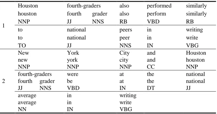
We will demonstrate the functioning of the POST STSS method on a pair of sentences from the Microsoft Research Paraphrase Corpus [33]. Table 1 contains the original sentences, their preprocessed and lemmatized forms, and their POS tag sequences.
Table 1. An example sentence pair from the Microsoft Research Paraphrase Corpus
1
Houston fourth-graders also performed similarly
houston fourth grader also perform similarly
NNP JJ NNS RB VBD RB
to national peers in writing
to national peer in write
TO JJ NNS IN VBG
2
New York City and Houston
new york city and houston
NNP NNP NNP CC NNP
fourth-graders were at the national
fourth grader be at the national
JJ NNS VBD IN DT JJ
average in writing
average in write
NN IN VBG
,
1
2
)
(
max
)
,
(
mn
n
m
S
S
R
P
These sentences were classified by human annotators as semantically different. Their meanings are actually rather similar, though worded differently, but the second sentence includes information about New York City students, which is not present in the first one. All system parameters used in this example are the ones gained by training our model on the training part of the Microsoft Research Paraphrase Corpus. We describe this training process in detail in Section 6.
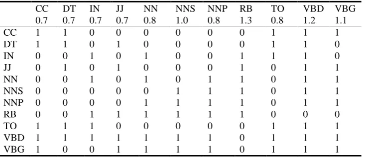
For the sake of convenience, we listed all POS weights used in this example and their respective POS interaction values in Table 2. The entire list of POS weights that our trained model utilizes is shown in Table 11, Section 7.3, while the entire configuration of the POS interaction matrix is given in Figure 1, in the same section. The chosen POS weighting function is the calculation of the arithmetic mean of the two POS weights.
Table 2. POS weights and POS interaction values used in this example
CC DT IN JJ NN NNS NNP RB TO VBD VBG
0.7 0.7 0.7 0.7 0.8 1.0 0.8 1.3 0.8 1.2 1.1
CC 1 1 0 0 0 0 0 0 1 1 1
DT 1 1 0 1 0 0 0 0 1 1 0
IN 0 0 1 0 1 0 0 1 1 1 0
JJ 0 1 0 1 0 0 0 1 0 1 1
NN 0 0 1 0 1 0 1 1 0 1 1
NNS 0 0 0 0 0 1 1 1 0 1 1
NNP 0 0 0 0 1 1 1 1 0 1 1
RB 0 0 1 1 1 1 1 1 0 0 0
TO 1 1 1 0 0 0 0 0 1 1 1
VBD 1 1 1 1 1 1 1 0 1 1 1
VBG 1 0 0 1 1 1 1 0 1 1 1
After preprocessing and lemmatization, the first sentence contains 11 tokens and the second 14. Hence, n = 14 and m = 11. There are 6 identical tokens in both sentences –
houston, fourth, grader, national, in, write. Therefore, d = 6.
The scores of these words depend only on their POS tag weights. If such a word has the same POS tag in both sentences, then its score is equivalent to the weight of its tag. Otherwise, its score is either equal to zero, if the pairing of the two different tags assigned to the word is prohibited, or is equal to the POS weighting function of its two tags, if the pairing of those tags is permitted.
To illustrate, the score of the word write is 1.1, since it appears in both sentences with a VBG tag, whose weight is 1.1. On the other hand, it could have been the case that in one of the sentences the word write appeared as a verb in the past tense (tag VBD), and in the other as a gerund/present participle (VBG). The POS interaction value for these two tags is one, meaning that their coupling is permitted. Since the weight of the VBD tag is 1.2 and the weight of the VBG tag is 1.1, the score of the word write would have been calculated as the arithmetic mean of these two values, which is 1.15.
The scores of all the words appearing in both sentences are then added up into a similarity sum Ssame. In this example, that sum would be Ssame = 5.0.
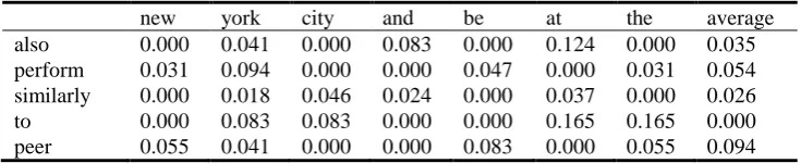
columns of the matrix represent words from the longer sentence. These matrices are: the string similarity matrix, shown in Table 3; the semantic similarity matrix, shown in Table 4; and the POS weighting matrix, shown in Table 5. The actual values in the matrices always depend on the particular words being considered. The semantic similarity scores also depend on the text corpus chosen to create the semantic space.
These matrices are then combined into a final similarity matrix, shown in Table 6. The values in each cell of the final matrix are calculated according to formula (1). Our trained model utilizes the same weight of 0.5 for both the string and the semantic similarity, which is also the value used in this example.
Table 3. The string similarity matrix
new york city and be at the average
also 0.000 0.041 0.000 0.083 0.000 0.124 0.000 0.035
perform 0.031 0.094 0.000 0.000 0.047 0.000 0.031 0.054
similarly 0.000 0.018 0.046 0.024 0.000 0.037 0.000 0.026
to 0.000 0.083 0.083 0.000 0.000 0.165 0.165 0.000
peer 0.055 0.041 0.000 0.000 0.083 0.000 0.055 0.094
Table 4. The semantic similarity matrix
new york city and be at the average
also -0.033 0.023 0.052 0.100 0.240 0.018 -0.003 -0.058
perform -0.097 -0.045 -0.031 0.225 0.031 0.106 -0.010 0.074 similarly -0.051 -0.070 -0.032 0.081 0.018 0.047 0.006 0.080
to -0.053 -0.142 -0.085 0.170 0.067 0.016 0.007 0.152
peer -0.052 -0.056 -0.101 0.149 0.071 -0.003 -0.063 0.025
Table 5. The POS weighting matrix
new york city and be at the average
NNP NNP NNP CC VBD IN DT NN
also RB 1.05 1.05 1.05 0.00 0.00 1.00 0.00 1.05
perform VBD 1.00 1.00 1.00 0.95 1.20 0.95 0.95 1.00
similarly RB 1.05 1.05 1.05 0.00 0.00 1.00 0.00 1.05
to TO 0.00 0.00 0.00 0.75 1.00 0.75 0.75 0.00
peer NNS 0.90 0.90 0.90 0.00 1.10 0.00 0.00 0.00
Table 6. The final similarity matrix
new york city and be at the average
also -0.017 0.034 0.027 0.000 0.000 0.071 0.000 -0.012
perform -0.033 0.024 -0.016 0.107 0.047 0.050 0.010 0.064 similarly -0.027 -0.027 0.008 0.000 0.000 0.042 0.000 0.056
to 0.000 0.000 0.000 0.064 0.033 0.068 0.064 0.000
We extract the best word pair from the final similarity matrix by finding the maximum-valued matrix element. We add the value of that element to a similarity sum
Sdifferent and then we remove the entire row and the entire column of that element from the matrix. The process is repeated as long as there are matrix rows left. The values extracted from the final similarity matrix are marked in bold script. The Sdifferent sum would in this case be Sdifferent = 0.383.
Our approach is based on a bag-of-words model, so it is incapable of pairing entire phrases, such as “similarly to national peers” and “at the national average”. However,
since our trained model mostly allows the pairings of words belonging to different parts of speech, it is able to pair the adverb “similarly” in the first phrase with the noun “average” in the second phrase, which is, arguably, the most appropriate choice here.
The final similarity score is found by using the formula (2) and its value is S(P, R) = 0.437. Our trained model utilizes a paraphrase detection threshold of 0.5, which means that this sentence pair has correctly been identified as one in which sentences are highly related, but not to the extent that they could be viewed as paraphrases. As an illustration, the score of this sentence pair would have been 0.519 had POS weighting not been used, leading to its misclassification by the system. This highlights the importance of POS weighting in giving a more realistic assessment of semantic similarity.
6.
Parameter Optimization
In order to obtain an optimal configuration of parameters for a given task, it is necessary to train the POST STSS model on a particular dataset. The optimization procedure must be performed only once for any given task, after which the system can function indefinitely using the obtained optimal parameters. Our training algorithm optimizes three types of parameters:
1. POS weights;
2. POS interaction matrix values;
3. Relative weights of the string and the semantic similarities.
We sought to keep the average similarity score around the mean value of 0.5 in an effort to prevent the general distribution of scores from becoming unbalanced. Since our model multiplies a similarity score by a weighting value, we used a POS weight range of [0.7, 1.3], which is both centered on the neutral value of one and symmetrical with regard to it. In effect, our POS weighting can increase or decrease the similarity score of a word pair by 30% at most. This particular choice was a trade-off between the preference for a broad range of weights and the need to keep the length of the training process manageable.
The relative weights of the string and the semantic similarities always add up to one. As a result, they can actually be optimized in terms of a single value in the range of [0, 1]. We chose to optimize the string similarity weight wstr while the semantic similarity weight wsem was calculated as wsem = 1 – wstr.
6.1. Dimensionality
The main problem in optimizing our model lies in its dimensionality. The Penn Treebank Project defined 36 different POS tags for the English language, which means that the POS interaction matrix contains 36 × 36 = 1296 cells. However, since semantic similarity is a symmetric relation, the POS interaction matrix is symmetric as well. Furthermore, it is logical to always permit the coupling of words belonging to the same part of speech, rendering the values along the main diagonal irrelevant. Consequently, there are 630 distinct binary values within the POS interaction matrix that ought to be determined. Taking into account the number of variables and their respective ranges of values, the size of the search space is given by the following expression:
11
2
7
36
630
Size
Space
Search
Full
(3)Clearly, an exhaustive search is impossible, given the enormous number of combinations. We tackled this problem by partially optimizing the parameters in a lower-dimensional search space and then continuing on from that semi-optimized point in the full-sized search space.
The lower-dimensional search space we used was based on aggregating several related POS tags into broader classes. We utilized six such categories:
1. Nouns – includes common nouns in the singular (NN) and the plural (NNS), as well as proper nouns in the singular (NNP) and the plural (NNPS). We also put nouns tagged as numerals (CD) in this category. Still, this does not include numeric tokens, since they are discarded in the preprocessing steps.
2. Verbs – includes verbs in their base form (VB), the past tense (VBD), and the present tense (VBP, VBZ), as well as present participles/gerunds (VBG), past participles (VBN), modals (MD), and particles (RP).
3. Adjectives – includes adjectives in their base (JJ), comparative (JJR), and superlative (JJS) forms.
4. Adverbs – includes adverbs in their base (RB), comparative (RBR), and superlative (RBS) forms, as well as Wh-adverbs (WRB).
5. Pronouns – includes personal (PRP) and possessive pronouns (PRP$), as well as their Wh- counterparts (WP, WP$).
6. Others – includes the remaining 12 tags (CC, DT, EX, FW, IN, LS, PDT, POS, SYM,
TO, UH, WDT).
The reasoning behind this approach is that the model should first be allowed to learn the relative importance of and interactions between general word classes. Only then should the focus shift toward the specificities of individual POS tags. For instance, it ought to be possible to detect whether, generally speaking, nouns are semantically more salient than adjectives and whether the pairing of these word classes in the context of STSS is sensible. These general conclusions can then be particularized with regard to the individual tags within these broader categories.
11
2
7
6
15
Size
Space
Search
Reduced
(4)Although this reduction significantly contains the combinatorial explosion, an exhaustive search still remains intractable. Therefore, our training procedure consists of the following two phases:
1. Pseudo-exhaustive searching in the lower-dimensional search space; 2. Steepest ascent hill climbing with momentum in the full-sized search space.
6.2. Pseudo-exhaustive Search
The idea of pseudo-exhaustive searching is to search exhaustively only among those parameter values which have some likelihood of being the optimal ones. We begin by choosing a single initial value for all POS weights, as well as a starting binary value for all the cells within the POS interaction matrix. An initial string similarity weight is also chosen. Finally, we select a POS weighting function among the five described in Section 5.3. We note the performance of the system on the training data with these initial settings, via a chosen metric.
We then explore all possible pairings of POS categories. We sequentially select a pairing and iterate over all combinations of POS weights for the word classes in the pair. While doing this, we fix to their initial values the weights of other word classes, the POS interaction matrix contents, and the string similarity weight. We then invert the POS interaction matrix bit of the pair that is being considered and repeat the process. In other words, we freeze the model in its initial state and only iterate over the changes of POS weights of the two given word classes and the changes of their respective POS interaction bit. Once a word class pairing has been explored, we reset the model to its initial state and start exploring another one. We do this for all possible pairings.
While iterating, we evaluate the model on the training data. For each pairing we note the POS weights and the respective POS interaction bit that maximized system performance. Since there are 15 different pairings possible in our lower-dimensional model, the size of the search space is quite manageable:
15
2
7
2
e Size
earch Spac
Pairing S
Word Class
(5)This approach presupposes that it is possible to accurately observe the interaction between two word classes in isolation. In effect, we assume that the choice of optimal weights and POS interaction bits for the entire model can be divided into a number of entirely separate decisions for each word class pairing. This assumption is obviously problematic, but it allows us to significantly reduce the search space and, ultimately, leads to promising results.
We then compile a list of candidate weights for each word class by going through the pairings in which it participated and collecting its optimal weights. The candidate values for each POS interaction matrix cell are simply the optimal POS interaction bit(s) from the respective word class pairing.
We exhaustively iterate over all combinations of candidate values for all POS weights and POS interaction bits. We do this while still keeping the string similarity weight fixed to its initial value. In each iteration we evaluate the model on the training data. At the end of the search we select those POS parameters which maximized system performance. The exact size of the search space in this stage is impossible to determine in advance, since it depends on the results of the previous step, but in our experience it can range from as low as 50 to as high as a couple of thousand. Nevertheless, this is still much smaller than the entire reduced search space whose size is on the order of ~1010.
In the final step of our pseudo-exhaustive search, we iterate over all possible values of the string similarity weight (from zero to one, with a step of 0.1) for each of the best-performing POS parameter sets from the previous stage. Since there are usually only one or two of them, this process is executed quickly. Again, in each iteration we evaluate the model on the training data. The full parameter combination(s) which maximized system performance is/are presented as the output of the pseudo-exhaustive search and is/are used as a starting point in the second phase of our training procedure – hill climbing.
We also experimented with applying a value minimization process to that output before starting the climb. The idea is that, depending on the set of initial conditions used in the search, certain POS weights might remain needlessly high and certain POS interactions might remain needlessly permitted, thereby obscuring the truly relevant POS interactions and weight values. To remedy this, our value minimization iterates over all POS weights and attempts to lower their values, if they are not already at the 0.7 minimum and if such changes do not diminish system performance on the training data. It also iterates over all bits of the POS interaction matrix and attempts to set them to zero, prohibiting the pairing of the respective word classes, if such modifications do not diminish system performance. The decision whether to use value minimization was one of the hyperparameters, which are described in the following subsection.
6.3. Hyperparameters
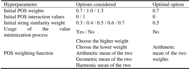
Hence, we divided the training data into three folds and repeatedly trained our model via a pseudo-exhaustive search on two of them and tested its final performance on the third while cyclically switching which fold is used for testing. We executed this procedure for all hyperparameter combinations. Finally, we adopted the combination that led to the best average test result on all three folds. In Table 7 we present a list of all hyperparameters, the different options we considered, and the optimal options that were chosen as final. The cross-validation was performed on the training portion of the Microsoft Research Paraphrase Corpus [33], which is described in detail in Section 7.
The selected POS weighting function is used not only during the pseudo-exhaustive search, but in the remainder of the training process and in the general functioning of the POST STSS method as well. Therefore, it can be regarded as a hyperparameter of the entire POST STSS model.
Table 7. Hyperparameters used in the pseudo-exhaustive search
Hyperparameter Options considered Optimal option
Initial POS weights 0.7 / 1.0 / 1.3 0.7
Initial POS interaction values 0 / 1 0
Initial string similarity weight 0.3 / 0.4 / 0.5 / 0.6 / 0.7 0.5
Usage of the value
minimization process Yes / No No
POS weighting function
Choose the higher weight Choose the lower weight Arithmetic mean of the two Geometric mean of the two Harmonic mean of the two
Arithmetic mean of the two weights
6.4. Steepest Ascent Hill Climbing
difference is that now this rule refers to individual parts of speech instead of broader word classes. Regardless, in such instances the POS interaction matrix is not consulted.
In the second phase of the training procedure we utilize a variation of the steepest ascent hill climbing algorithm. As the full-sized space is so large, hill climbing is one of the few viable options. We employ three kinds of moves:
1. An increase/decrease of a single POS weight;
2. An inversion of a single bit within the POS interaction matrix; 3. An increase/decrease of the string similarity weight.
In each step of the climb we evaluate the effect of every possible move on the entire training data. The typical steepest ascent reasoning would be to select the move which leads to the largest increase in system performance. Instead of always following this logic, we add a momentum to each move which alters the string similarity weight or a POS weight. If a certain weight change has the largest positive impact on system performance, then it is perpetuated as long as the performance keeps increasing, even if, at some point, there appears another move which would lead to a greater performance increase. The momentum feature allows our algorithm to escape from certain local maxima and not only leads to better final results, but speeds up the hill climb as well. Once the repeated weight increase/decrease no longer improves system performance, we resume the climb using the standard steepest ascent method.
To speed up the climb, we allow a move which alters a POS weight to simultaneously invert one POS interaction bit. This added inversion is permitted only on the bits that pertain to the POS whose weight is being modified. Furthermore, we allow the climb to include jumps – moves in which a weight is changed not by the usual step of 0.1, but by twice as much. We also let the POS weight jumps to invert a related POS interaction bit. If multiple moves lead to the same level of performance improvement, our algorithm randomly picks one of them. Thus, each run of the climb can produce different results. This allows multiple runs of our algorithm to explore a larger portion of the search space than would have otherwise been the case.
The hill climbing can be sustained as long as there are moves which lead to better performance on the training data. However, this would likely result in an overfitted model. To prevent this, we used a simple heuristic – we first ran the hill climbing algorithm several times, finishing the climb only when all the moves leading to superior system performance are exhausted. In each run we noted how many moves it took to reach that final stage. Our analysis showed that the maximum length of this process is around 50 moves. We chose to stop the climb after 25 moves, i.e. half of the maximum. Although this heuristic is rather crude, it actually performed quite well in practice. Therefore, the parameters acquired after 25 moves are the ones we adopt as final. They are used in the evaluation of the POST STSS method described in Section 7.
If a certain hyperparameter combination leads to multiple starting points for the hill climb, we can simply repeat the climb from each point. Then we can pick the final parameter combination which performs best on the training data. However, this situation did not occur with our optimal hyperparameter options.
Although our training procedure is not guaranteed to find the global optimum, it still leads to good results. One of main strengths of the proposed training algorithm is that almost all of its stages can be effectively parallelized, leading to a significant reduction in the length of the procedure.
7.
Evaluation
We evaluated our model by using a paraphrase recognition test on the Microsoft
Research Paraphrase Corpus (MSRPC) [33]. The MSRPC is a corpus containing 5801
pairs of sentences which are all semantically related to some extent. However, only some sentence pairs are paraphrases, i.e. semantically equivalent, while others have only partly overlapping semantic information. The entire corpus was hand-annotated with binary scores indicating for each pair if it is a paraphrase or not. 3900 pairs (67%) were deemed semantically equivalent, while the remaining 1901 (33%) were classified as semantically diverse. Two human raters examined each pair, while a third cast the deciding vote in cases of disagreements. The average inter-rater agreement was 83%, which is therefore the maximum accuracy an STSS system can reach.
The task of STSS systems is to match the sentence-pair scores of human annotators, thereby testing the systems’ ability to accurately assess the level of semantic similarity between two sentences. To do so, a threshold between zero and one has to be chosen, so that any score above it is treated as recognition of semantic equivalence and any below it as indication of semantic divergence.
The MSRPC dataset was originally split into a training portion consisting of 4076 sentence pairs, and a test portion encompassing 1725 pairs. The training part is used to determine the optimal threshold value, while the evaluation is performed on the testing part. We changed the threshold in 0.1 increments in order to limit the possibility of overfitting to the training data. In addition, we used the training set in the parameter optimization process described in the previous section. During training, a new optimal threshold value was determined whenever a performance evaluation was required. This was done so as to maximize system performance at each point in the process.
7.1. Performance Metrics
However, there are other metrics, taken from the information retrieval theory, which are also frequently employed. Precision is the ratio of true positives and all pairs classified as paraphrases. Therefore, precision reflects the level of false positive errors, while ignoring false negative ones. Recall is calculated as the ratio of true positives and all paraphrase pairs from the corpus. Recall measures the level of false negatives, but ignores the false positive errors. This is why it is easy to optimize a system to have either high precision or high recall, at the expense of the other. The F-measure was introduced as a standard way of combining these measures into a unified, balanced score, and is defined as the harmonic mean of precision and recall. The mathematical formulas for calculating all these metrics are given by the following expressions:
FN
TN
FP
TP
TN
TP
A
(6)FP
TP
TP
P
(7)FN
TP
TP
R
(8)R
P
PR
F
2
(9)As shown in expressions 7–9, the F-measure fails to take into account the level of true negatives an STSS system produces. This makes accuracy the predominant parameter of system evaluation since it measures not only false positive and false negative types of errors, but also the level of performance on both true positives and true negatives. Such a broad scope of evaluation is essential for problems in which the level of true negatives is not to be ignored. This is the case in all situations where measuring semantic dissimilarity is important (e.g. in extractive text summarization STSS is used to calculate semantic dissimilarity between the already selected summary sentences and a set of potential candidates). Thus, we decided to train the model and to pick the optimal threshold value according to the maximal system accuracy.
7.2. Results
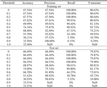
An overview of POST STSS behavior on the MSRPC paraphrase recognition test with regard to different threshold values is given in Table 8. As shown, the optimal threshold value for our system is 0.5.
Some previously devised methods were presented in a number of variants. In such cases, the version with the highest accuracy was chosen for comparison. Lintean and Rus [13] presented both a topological and a statistical similarity variant of their approach, so we included both in the table.
In addition, we implemented a slight modification of the LInSTSS approach of Furlan et al. [20] which does not use stop-word removal. This was done in order to compare that algorithm to our own on equal terms, since our model does not use a stop-word list. The LInSTSS implementation utilized the same text corpus and stemming technique described in Section 4.
Table 8. An overview of POST STSS performance on the MSRPC paraphrase recognition test with regard to different threshold values
Threshold Accuracy Precision Recall F-measure
Training set
0 67.54% 67.54% 100.00% 80.63%
0.1 67.54% 67.54% 100.00% 80.63%
0.2 67.57% 67.56% 100.00% 80.64%
0.3 67.62% 67.61% 99.93% 80.65%
0.4 69.09% 69.01% 98.44% 81.14%
0.5 74.34% 75.87% 90.92% 82.72%
0.6 68.40% 82.69% 67.31% 74.21%
0.7 53.70% 92.62% 34.18% 49.93%
0.8 36.21% 97.52% 5.70% 10.78%
0.9 32.56% 100.00% 0.15% 0.29%
1.0 32.46% NaN 0% NaN
Test set
0 66.49% 66.49% 100.00% 79.87%
0.1 66.49% 66.49% 100.00% 79.87%
0.2 66.49% 66.49% 100.00% 79.87%
0.3 66.55% 66.53% 100.00% 79.90%
0.4 68.87% 68.46% 98.61% 80.81%
0.5 74.09% 75.74% 89.80% 82.17%
0.6 66.78% 81.89% 64.25% 72.01%
0.7 51.42% 88.92% 30.78% 45.73%
0.8 36.93% 96.83% 5.32% 10.08%
0.9 33.51% NaN 0% NaN
1.0 33.51% NaN 0% NaN
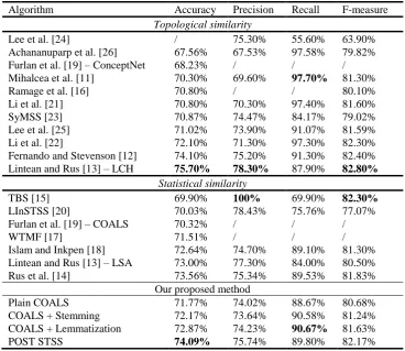
The POST STSS method outperforms the current state-of-the-art statistical similarity algorithms in terms of accuracy. Its F-measure is also higher than most other statistical solutions. Only TBS [15], a topic modeling approach, performs slightly better in terms of the F-measure, but with a considerably lower accuracy. The topological similarity measures of Fernando and Stevenson [12] and Lintean and Rus [13] attain similar or better results than we do, but at the cost of having to use a hand-crafted knowledge base in the form of WordNet. This makes their solutions unsuitable for a broad range of languages in which such resources are nonexistent. Moreover, the POST STSS method achieves a significantly better accuracy than all structural models, including the algorithms ([19], [21], [22], [23]) which employ a weighting mechanism in conjunction with (shallow) parsing and/or semantic role labeling to detect constituents. This result validates our view that POS tags are well suited to be used in such weighting schemes as indicators of the deeper syntactic information.
Table 9. A comparison between the results of the existing STSS solutions and our proposed method on the MSRPC paraphrase recognition test
Algorithm Accuracy Precision Recall F-measure
Topological similarity
Lee et al. [24] / 75.30% 55.60% 63.90%
Achananuparp et al. [26] 67.56% 67.53% 97.58% 79.82%
Furlan et al. [19] – ConceptNet 68.23% / / /
Mihalcea et al. [11] 70.30% 69.60% 97.70% 81.30%
Ramage et al. [16] 70.80% / / 80.10%
Li et al. [21] 70.80% 70.30% 97.40% 81.60%
SyMSS [23] 70.87% 74.47% 84.17% 79.02%
Lee et al. [25] 71.02% 73.90% 91.07% 81.59%
Li et al. [22] 72.10% 71.30% 97.30% 82.30%
Fernando and Stevenson [12] 74.10% 75.20% 91.30% 82.40%
Lintean and Rus [13] – LCH 75.70% 78.30% 87.90% 82.80%
Statistical similarity
TBS [15] 69.90% 100% 69.90% 82.30%
LInSTSS [20] 70.03% 78.43% 75.76% 77.07%
Furlan et al. [19] – COALS 70.32% / / /
WTMF [17] 71.51% / / /
Islam and Inkpen [18] 72.64% 74.70% 89.10% 81.30%
Lintean and Rus [13] – LSA 73.00% 77.30% 84.00% 80.50%
Rus et al. [14] 73.56% 75.34% 89.53% 81.83%
Our proposed method
Plain COALS 71.77% 74.02% 88.67% 80.68%
COALS + Stemming 72.17% 73.64% 90.58% 81.24%
COALS + Lemmatization 72.87% 74.23% 90.67% 81.63%
POST STSS 74.09% 75.74% 89.80% 82.17%
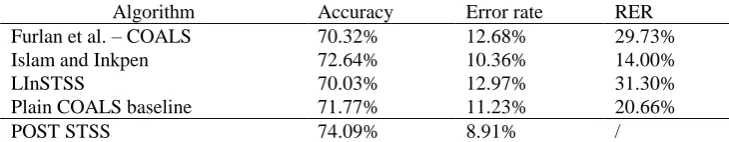
comparison, alongside our Plain COALS baseline, are shown in Table 10. We also included the LInSTSS algorithm [20] in the comparison, because it is a modification of the same two methods we used as our starting point. We presented the error rates of all algorithms, given that the maximal possible accuracy on the task is 83%. In addition, we calculated the relative error reduction of our approach, when compared to the existing solutions and our baseline. The relative error reduction is computed as:
ES
STSS POST ES
Error
Error
Error
RER
(10)where Error ES is the error rate of one of the existing solutions or the baseline, and Error
POST STSS is the error rate of the POST STSS method.
Table 10. Improvements of the POST STSS method with regard to related methods and the existing solutions which were used as a starting point for our approach
Algorithm Accuracy Error rate RER
Furlan et al. – COALS 70.32% 12.68% 29.73%
Islam and Inkpen 72.64% 10.36% 14.00%
LInSTSS 70.03% 12.97% 31.30%
Plain COALS baseline 71.77% 11.23% 20.66%
POST STSS 74.09% 8.91% /
Surprisingly, the LInSTSS approach actually performed the worst. We found several factors which could have had a detrimental effect on it. To begin with, in order to avoid overfitting to the training data we had decided to use a 0.1 increment when searching for the optimal threshold. This did not degrade the performance of POST STSS since the values of the POS weights it uses also change in steps of 0.1, i.e. rather coarsely. On the other hand, the method of term frequency weighting implemented in LInSTSS uses a finely differentiated range of weights between 0.5 and 1.0. This means that the 0.1 step is much too coarse for choosing a threshold in LInSTSS. We tested this hypothesis by lowering the threshold step to 0.001, as was suggested by Furlan et al. [20]. The results validated our finding since the accuracy rose to 71.48%.
7.3. Optimal Parameters
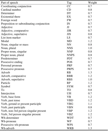
The final results of the POST STSS method were achieved by using the POS weights shown in Table 11. Entries in the table are sorted alphabetically according to their POS tag [8]. We obtained these specific weights by training the model on the MSRPC training set in the manner described in Section 6. The final optimal weights for the string and the semantic similarities were both 0.5.
Table 11. Optimal part-of-speech weights
Part of speech Tag Weight
Coordinating conjunction CC 0.7
Cardinal number CD 0.8
Determiner DT 0.7
Existential there EX 0.7
Foreign word FW 0.7
Preposition or subordinating conjunction IN 0.7
Adjective JJ 0.7
Adjective, comparative JJR 0.7
Adjective, superlative JJS 0.8
List item marker LS 0.7
Modal MD 1.2
Noun, singular or mass NN 0.8
Noun, plural NNS 1.0
Proper noun, singular NNP 0.8
Proper noun, plural NNPS 0.8
Predeterminer PDT 0.7
Possessive ending POS 0.7
Personal pronoun PRP 0.7
Possessive pronoun PRP$ 0.7
Adverb RB 1.3
Adverb, comparative RBR 1.2
Adverb, superlative RBS 1.0
Particle RP 1.2
Symbol SYM 0.7
To TO 0.8
Interjection UH 0.7
Verb, base form VB 1.2
Verb, past tense VBD 1.2
Verb, gerund or present participle VBG 1.1
Verb, past participle VBN 0.8
Verb, non-3rd person singular present VBP 1.2
Verb, 3rd person singular present VBZ 1.2
Wh-determiner WDT 0.7
Wh-pronoun WP 0.7
Possessive wh-pronoun WP$ 0.7
Our system gives the highest weight to verbs and adverbs, reflecting the claim of Wiemer-Hastings that humans are more strongly affected by the similarities of verbs than that of the other constituents [27]. This also corresponds to the findings of other researchers ([19], [23]) who showed that actions, i.e. verbs, are semantically more salient than subjects/objects involved in them. Interestingly, it is two of the adverb tags (RB and WRB) that actually have the highest weight assigned to them. Apart from the inherent importance of adverbs as modifiers of verbs, this effect likely stems, at least in part, from the distribution of examples in the paraphrase corpus. The MSRPC contains numerous instances where both sentences in a pair describe the same basic action but performed in different manners. In such situations giving more weight to adverbs is an elegant way of detecting these dissimilarities.
In addition to verbs and adverbs, nouns are also given higher weights than most other parts of speech. This showcases their syntactic significance since nouns often play the roles of subjects and objects in a sentence. The remaining parts of speech are mostly given lower weights, indicating their reduced impact on STSS due to the limited amount of semantic information they carry.
The optimal POS interaction matrix configuration is depicted in Figure 1. Values within it are ordered according to the alphabetical ordering of tags in both the left-to-right and the top-to-bottom direction [8]. Therefore, the first row and the leftmost column correspond to the tag CC, while the last row and the rightmost column correspond to the tag WRB. A value of one means that the pairing of the parts of speech that correspond to a particular row and column is permitted. A value of zero means that such a coupling is forbidden.
Even though the starting value of all matrix cells was zero, as set via a hyperparameter described in Section 6.3, the final matrix mainly contains values of one. This means that disallowing the pairing of words with different POS tags can be beneficial only in a limited number of situations. Hence, the impact of POS weights is even larger, since most POS interactions are allowed.
Most values are grouped in uniform rectangular portions of the matrix, since they were chosen jointly, by allowing/disallowing pairings on the level of broader word classes. Many groupings have a linguistically understandable backing, if considered within a bag-of-words model. For instance, verbs can be paired with any word class except for adverbs. Nouns can, in general, only be paired with verbs and adverbs. Most adjectives cannot be paired with nouns and words in the “other” category. It is permitted to pair adverbs with adjectives, nouns, and pronouns, but not with verbs and words in the “other” category. There are also certain matrix values that are somewhat surprising. For example, pronouns can be paired with any word class, except for nouns. Since nouns and pronouns often have similar syntactic roles, this indicates that aligning words solely on the basis of their syntactic properties might not be the correct choice for STSS, at least within a bag-of-words model. Finally, words in the “other” category can be paired with pronouns and verbs. Of course, words within a broader word class can, by and large, be paired with other words in the same class.
performance. Such fine-grained decisions are made during the hill-climbing part of the training process, described in Section 6.4.
1 0 1 1 1 0 0 0 0 1 1 0 0 0 0 1 1 1 1 0 0 0 1 1 1 1 1 1 1 1 1 1 1 1 1 0 0 1 0 0 0 0 0 0 0 0 1 1 1 1 1 0 0 0 0 1 1 1 1 0 0 0 1 1 1 1 1 1 0 0 0 1 1 0 1 1 1 0 1 0 0 1 1 0 0 0 0 1 1 1 1 0 0 0 1 1 1 1 1 1 0 1 1 1 1 1 1 0 1 0 1 1 1 0 0 0 0 1 1 0 0 0 0 1 1 1 1 0 0 0 1 1 1 1 1 1 1 1 1 1 1 1 1 0 1 0 1 1 1 1 0 0 0 1 1 0 0 0 0 1 1 1 1 0 0 0 1 1 1 1 1 1 1 1 1 1 1 1 1 0 0 0 0 0 1 1 0 0 0 1 0 1 0 0 0 1 1 1 1 1 1 0 1 1 1 1 1 1 0 1 1 0 1 0 1 0 0 0 1 0 0 0 1 1 0 0 1 0 0 0 0 0 0 1 1 1 1 1 1 0 0 0 1 1 1 1 1 1 0 1 1 1 0 0 0 0 0 0 1 1 1 0 1 0 0 0 0 0 0 1 1 1 1 1 1 0 0 0 1 1 1 1 1 1 0 1 1 1 0 0 0 0 0 0 0 1 1 0 1 0 0 0 0 0 0 1 1 1 1 1 1 0 0 0 1 1 1 1 1 1 0 1 1 1 1 0 1 1 1 1 0 0 0 1 1 0 0 0 0 1 1 1 1 0 0 0 1 1 1 1 1 1 1 1 1 1 1 1 1 0 1 1 1 1 1 0 1 1 1 1 1 0 1 1 1 1 1 1 1 0 0 0 1 1 1 1 1 1 1 1 1 1 1 1 1 0 0 1 0 0 0 1 0 0 0 0 0 1 0 1 1 0 0 0 0 1 1 1 1 0 0 0 1 1 1 1 1 1 0 0 0 1 0 1 0 0 0 0 0 0 0 0 1 0 1 1 1 0 0 0 0 1 1 1 1 0 0 0 1 1 1 1 1 1 0 0 0 1 0 1 0 0 0 0 0 0 0 0 1 1 1 1 1 0 0 0 0 1 1 1 1 0 0 0 1 1 1 0 1 1 0 0 0 1 0 1 0 0 0 0 0 0 0 0 1 1 1 1 1 0 0 0 0 1 1 1 1 0 0 0 1 1 1 1 1 1 0 0 0 1 1 0 1 1 1 1 0 0 0 1 1 0 0 0 0 1 1 1 1 0 0 0 1 1 1 1 1 1 1 1 1 1 1 1 1 0 1 0 1 1 1 1 0 0 0 1 1 0 0 0 0 1 1 1 1 0 0 0 1 1 1 1 1 1 1 1 1 1 1 1 1 0 1 0 1 1 1 1 1 1 1 1 1 0 0 0 0 1 1 1 1 1 1 1 1 1 1 1 1 1 1 1 1 1 1 0 1 1 1 0 1 1 1 1 1 1 1 1 1 0 0 0 0 1 1 1 1 1 1 1 1 1 1 1 1 1 1 1 1 1 1 1 1 1 0 1 0 0 0 1 1 1 1 0 0 1 1 1 1 0 0 1 1 1 1 0 0 0 0 0 0 0 0 1 0 0 0 1 1 1 0 1 0 0 0 1 1 1 1 0 0 1 1 1 1 0 0 1 1 1 1 1 0 0 0 0 0 0 0 0 0 0 0 1 1 1 0 1 0 0 0 0 1 1 1 0 0 1 1 1 1 0 0 1 1 0 1 1 0 0 0 0 0 0 0 0 0 0 0 1 1 1 1 1 1 1 1 1 1 1 1 1 1 1 1 1 1 1 1 1 1 0 0 0 1 1 1 1 1 1 1 1 1 1 1 1 1 0 1 0 1 1 1 1 0 0 0 1 1 0 0 0 0 1 1 1 1 0 0 0 1 1 1 1 1 1 1 1 1 1 1 1 1 0 1 0 1 1 1 1 0 0 0 1 1 0 0 0 0 1 1 1 1 0 0 0 1 1 1 1 1 1 1 1 1 1 1 1 1 0 1 0 1 1 1 1 0 0 0 1 1 0 0 0 0 1 1 1 1 0 0 0 1 1 1 1 1 1 1 1 1 1 1 1 1 0 1 1 1 1 1 1 1 1 1 1 1 1 1 1 1 1 1 1 1 0 0 0 1 1 1 1 1 1 1 1 1 1 1 1 1 0 1 1 1 1 1 1 1 1 1 1 1 1 1 1 1 1 1 1 1 0 0 0 1 1 1 1 1 1 1 1 0 1 1 1 1 0 1 1 0 1 1 0 1 1 1 1 1 1 1 1 1 1 1 1 1 0 0 0 1 1 1 1 1 1 1 1 1 0 1 1 1 0 1 1 1 1 1 1 1 1 1 1 1 1 1 0 1 1 1 1 1 1 0 0 1 1 1 1 1 1 1 1 1 1 1 1 1 0 1 1 1 1 1 1 1 1 1 1 1 1 1 1 1 1 1 1 1 0 0 0 1 1 1 1 1 0 1 1 1 1 1 1 1 0 1 1 1 1 1 0 1 1 1 1 1 1 1 1 1 1 1 1 1 0 0 0 1 1 1 1 1 1 0 1 1 1 1 1 1 0 1 0 1 1 1 1 0 0 0 1 1 0 0 0 0 1 1 1 1 0 0 0 1 1 1 1 1 1 1 1 1 1 1 1 1 0 1 0 1 1 1 0 1 1 1 1 1 0 0 0 0 1 1 0 1 1 1 1 1 1 1 1 1 1 1 1 1 1 1 1 1 1 1 0 1 1 1 1 1 1 1 1 1 0 0 0 0 1 1 1 1 1 1 1 1 1 1 1 1 1 1 1 1 1 1 1 1 1 0 1 0 0 0 0 1 1 1 0 0 1 1 1 1 0 0 1 1 1 1 1 0 0 0 0 0 0 0 0 0 0 0 1 1 1
8.
Conclusion
In this paper we have presented POST STSS, a bag-of-words approach to measuring the semantic similarity of short texts based on using part-of-speech tags as indicators of the deeper syntactic information. We have described our proposed system’s operation, including the central POS tag weighting technique, as well as the parameter optimization procedure. We have trained the model and evaluated its performance by using a paraphrase corpus. We have concluded that our method achieves a higher accuracy than current state-of-the-art statistical similarity algorithms. In this respect it also outperforms the methods which utilize more advanced syntax-processing tools. Since our approach does not require either hand-crafted knowledge bases or advanced syntactic tools like parsers and semantic role labelers, it is more easily applicable to languages with scarce natural language processing resources.
A potential avenue of future research could focus on integrating our POS weighting strategy with shallow parsing, which groups several words/POS tags into noun, verb, or preposition phrases. By weighting both the phrases and the POS tags within them, it may be possible to develop an even better representation of the relative semantic importance of different constituents.
An alternative research direction would be the verification of o