Using Energy Efficient Ethernet (802.3az) in Web Hosting Centers

(1)

III

UN

IV

E

R S

I

D

A

D · C

A R_{L O S} I II ·

DE

M

A

D

R

ID

:

UNIVERSITY CARLOS III OF MADRID

Department of Telematics Engineering

Master of Science Thesis

Using Energy Efficient Ethernet (802.3az) in Web Hosting

Centers

Author: Angelos Chatzipapas

Dipl. Eng. in Computer Engineering and Informatics

Supervisors: Antonio de la Oliva, Ph.D. Vincenzo Mancuso, Ph.D.

(2)

Abstract

The contribution of this master thesis is twofold. First we present an analytical model of IEEE 802.3az and second we summarize the results of our measurement campaign con-ducted in collaboration between Institute IMDEA Networks and InterHost. The analytical model uses simple traffic parameters to estimate the power consumption of the newly re-leased standard for Energy Efficient Ethernet (EEE), namely IEEE 802.3az. With our mea-surements, we have characterized the behavior of the aggregate traffic flowing through one of the InterHost company’s firewalls at one of their web hosting centers located in Madrid, Spain. We used the collected data in order to evaluate the potential for power saving that could be achieved by replacing the company’s gigabit wired links with EEE connections. In the thesis, we plot the daily load and the potential power saving computed by simulat-ing the measured traffic with an EEE link simulator as well. Ussimulat-ing the presented model for predicting the EEE power saving from few statistical traffic parameters, we show that the EEE power saving for 1000Base-T links can be estimated with good accuracy. Finally, to show the importance of precise measurements, we first collect high precision timestamps for packet arrivals by means of specialized high resolution hardware, then we post-process the collected traces and introduce uniformly distributed random noise to the original times-tamps. Results show that(i)substantial power saving could be achieved, higher that 40% in the peak hour and as high as 90% overnight, and that(ii)EEE power saving predictions can be biased by timestamp errors and so, high precision hardware is needed. Last but not least, packet coalescing for EEE is discussed to further reduce the power consumption of links under medium to high load operation.

(3)

Table of Contents

1 Introduction 1

2 Energy Efficient Ethernet - (EEE) 3

2.1 Behavior of EEE Links . . . 3

3 Analytical Model 6 3.1 1GbpsUnidirectional EEE Links . . . 7

3.2 100M bpsand10GbpsUnidirectional EEE Links . . . 9

3.3 Deriving Model Parameters from Measurements . . . 10

4 Energy Efficiency in Web Hosting Centers 11 4.1 Motivation . . . 11

4.2 Unintrusive Measurements at InterHost . . . 12

4.3 Using the Collected Traces (EEE Simulation and Model) . . . 13

4.4 Traffic Behavior and EEE Power Saving . . . 13

4.5 Zooming over the Weekly Saving . . . 14

4.6 Impact of Noisy Measurements . . . 15

5 Related Proposals 18 5.1 Evaluation of EEE . . . 18

5.1.1 Model . . . 18

5.1.2 Simulation Results . . . 18

5.1.3 Performance Measurements of Real Cards . . . 20

5.2 Boosting Energy Efficiency with Packet Coalescing . . . 21

6 Conclusions 23

(4)

List of Figures

2.1 State transition diagrams for various link speeds. . . 4

2.2 Channel transitions during a whole cycle. . . 4

3.1 System cycle for EEE links. . . 7

4.1 Measurement tools. . . 12

4.2 The power savings during a whole month. . . 14

4.3 Weekly plots. . . 15

4.4 Noise introduction. . . 16

5.1 Power consumption vs. Load (data from [4]). . . 19

5.2 Impact of coalescing on power save and on delay (data from [18]). . . 22

(5)

Chapter 1

Introduction

During the past years a lot of effort has been made to increase processing, communica-tion, switching speed and data storage without any effort to optimize the power consumption. According to [1], about14 T W hwere consumed in 2005 by the telecom core network in EU-251 and the consumption is expected to increase to about 30T W h by 2020. We can understand that, although this power consumption is useful for the human beings, it is also potentially harmful for our environment since it produces an augmented amount of CO2

emissions and highly contributes to the greenhouse effect. The current threat to the environ-ment could turn into a much more serious threat in the near future, since there is a growing demand of new generation devices that require connection to the Internet (such as televi-sions, white goods, etc.). In addition existing network connected devices are now increasing their bandwidth demands (e.g., Web servers, databases, etc.). In fact, the Internet traffic might grow with the number of data centers in the network and the number of users that demand higher amounts of traffic such as bigger files, videos, TV over IP etc. Hence, as the demand for much traffic rises, especially in developing countries, more and more energy consumption is expected for networking.

In order to protect the environment and obtain lower service cost, Internet Service Providers (ISPs) and network operators are currently trying to deploy new strategies to achieve lower energy bills and reduced energy consumption. There are three main roadmaps to achieve these goals:

1. The hardware optimization using more efficient electronics in order to reduce the power consumption of the components (the hardware producers are responsible for it).

2. The rising usage of renewable power sources (solar panels, wind generator etc.).

3. The use of power saving models and energy efficient algorithms (ISPs and network operators are responsible for it).

1_{The first 25 European countries that were forming European Union at that period: Austria, Belgium, Cyprus,} Czech Republic, Denmark, Estonia, Finland, France, Germany, Greece, Hungary, Ireland, Italy, Latvia, Lithua-nia, Luxembourg, Malta, Poland, Portugal, Slovakia, SloveLithua-nia, Spain, Sweden, The Netherlands, United King-dom

(6)

2 Chapter 1. Introduction

This thesis investigates to the third roadmap, using the recently approved Energy Ef-ficient Ethernet (EEE) standard for power saving issues in Local Area Networks. Indeed, according to [2], based on estimations for the year 2005, EEE can potentially obtain signifi-cant reductions of about3T W hper year.

Legacy Ethernet is a power-unaware standard which consumes a constant amount of power independently on the actual traffic, flowing through the wires. However, low speed Ethernet cards consume about200mW which is not significant considering the power con-sumption of a server or a home PC, so that Ethernet power saving strategies were not relevant for low speed connections. In contrast, new high speed Gigabit interface cards may consume up to20W which makes reasonable the introduction of a power saving mechanism. In fact, taking into account that the amount of Web Hosting Centers and server farms has been ex-tremely increased due to the new trends and services (YouTube, Facebook, Twitter etc.), there are now billions of running interfaces that consume a constant amount of power. In ad-dition, Ethernet links are basically inactive most of the time. Therefore, a new power aware Ethernet standard (standardized late 2010) was introduced to minimize the power consump-tion of the links, namely IEEE 802.3az, or EEE (Energy Efficient Ethernet).

Later in this thesis, we present an analytical model, that uses simple statistical parame-ters, (such as mean interarrival time, variance etc.) and models the power consumption of an EEE link over time. We use real traces to evaluate the potential EEE power saving, and we focus exclusively on1Gbpslinks, which are the most widely adopted ones, and on the impact of uplink/downlink traffic correlation on such saving. With our results we show that EEE might save more than 40% of the link power most of the time, with peaks of 90% or more during night hours. We also unveil that high precision packet timestamps are key to achieve high accuracy estimations via simulation, and to enable the use of simplified ana-lytical computations. In particular, noisy measurements severely impact the quality of EEE power saving estimates as soon as the maximum timestamp deviation due to noise reaches a few milliseconds, which is below the typical timestamp accuracy of non-dedicated net-work hardware, i.e., of inexpensive but imprecise driver timestamping. This justifies using specialized high accuracy timestamping hardware.

(7)

Chapter 2

Energy Efficient Ethernet - (EEE)

Energy Efficient Ethernet 802.03az [3] was standardized in September 2010 and aims to provide significant power saving in LANs. Formerly, the evolution of LANs led towards higher link speeds for faster communication and higher bandwidth, in order to satisfy the in-creased demand for data (link speeds from10M bpsto10Gbps). The electricity consump-tion of relatively “old” network interfaces remained in very low levels so the main concern of Ethernet component producers was not to save power. For example, in100M bps Eth-ernet links, the EthEth-ernet devices consume about200mW of power [4]. However, the new high speed Ethernet (1Gbpsor faster) requires several Watts of power consumption [5] for each interface. Considering a usual server that consumes around200W, a simple Ethernet device contributes to 10% of this amount. Indeed, data and Web Hosting Centers have a huge number of interface cards which finally generate a high cost for the center (electricity bills). Thus, the idea of reducing the power consumption of Ethernet links appears in the foreground.

Legacy Ethernet consumes a constant amount of power with or without traffic which makes it totally inefficient with typical Ethernet traffic profiles. This behavior results in a huge waste of power since it is well known that Ethernet links are inactive most of the time with utilization factors from 5% for a home PC to 30% for heavy loaded data servers [6–8]. EEE aims to reduce this waste of power and approach power proportionality, i.e., a power consumption proportional to the served traffic. The EEE standard introduces four new states for the links, state “Active” (A) which represents the busy period, state “Low Power Idle” (LPI) in which there is no traffic and the link consumes 90% less power that in state A according to measurements [9], and states “Sleep” (S) and “Wake Up” (W) which correspond to the time spent during switching from state A to LPI and vice versa, respectively [10]. In the following subsection, we describe how EEE links behave.

2.1

Behavior of EEE Links

The behavior of EEE links is illustrated in Fig. 2.1. Packet transmissions may occur only in state A. When there is no traffic to serve, the link switches to LPI state, where it consumes about 10% of the power consumption in state A [9]. The transition intervalTS

between states A and LPI is denoted as the state S of the link. When a new frame arrives in either side of the link for transmission, the link switches back to state A after a transition

(8)

4 Chapter 2. Energy Efficient Ethernet - (EEE)

(a) State transition diagram for 100Base-T and 1000Base-T EEE links.

(b) State transition diagram for 10GBase-T EEE links.

Figure 2.1: State transition diagrams for various link speeds.

Figure 2.2: Channel transitions during a whole cycle.

timeTW which defines the state W of the link. According to EEE, the duration ofTS and

TW varies among the different link speeds. Table 2.1, indicates the duration of the two states

for 100Base-Tx, 1000Base-T and 10GBase-T links. The table also shows the transmissions time and the efficiency (the time to transmit a frame over the time to transmit a frame plus

TW +TS) for a whole cycle of a big and a small frame. Furthermore, the standard defines a

“Refresh” message, that checks the channel state in LPI, ensures that the receiver elements still follow the channel conditions and maintains the duration ofTW in low levels. Fig. 2.2 shows the channel state transitions over time for a whole cycle (note that an LPI interval is composed by several idle intervalsTqand refresh intervalsTr).

Table 2.1: Time required for W, S and Frame Transmission [µs]

Speed Minimum Minimum Transm. time Transm. time

TS TW for1500bytes for150bytes

frame (efficiency) frame (efficiency) 100Base-T 200 30 120 (48%) 12 (4.8%) 1000Base-T 182 16 12 (5.7%) 1.2 (0.57%)

10GBase-T 2.88 4.48 1.2 (14.6%) 0.12 (1.46%)

(9)

5 Chapter 2. Energy Efficient Ethernet - (EEE)

direction can go to LPI independently of the traffic activity in the other direction. In contrast, in 1000Base-T links, EEE can enter in state LPI only when both link directions have no data to send. Second, 100Base-Tx and 1000Base-T links treat differently a new frame that arrives during state S than 10GBase-T links. As illustrated in the transition diagrams in Fig. 2.1b,

10GbpsEEE links have to execute the whole sequence of states S-LPI-W before switching back to the state A, while in Fig. 2.1a,100M bpsand1000M bpsEEE links in state S can switch directly to state A if there is a new packet arrival.

At this point, it is important to mention that, in states S and W, EEE links practically consume as much power as in state A (see to Reviriego et al. [9]). So, the actual EEE saving is obtained when the link remains in state LPI. As a consequence, the goal of most research studies is to find how the links can remain in state LPI for the longest possible duration.

(10)

Chapter 3

Analytical Model

We model the behavior of the EEE link as anM/G/1queue in which the packet service rate is non-zero only in state A, where it equals a constantR, corresponding to the link speed. We denote bySp the size of a single packet and byE[Sp]the average packet size. Frames

arrive in batches of random sizeNb≥1packets, according to a Poisson process with rate

λ[11]. Arrivals in batches simulate as much as possible the behavior of real networks, since usually packets arrive at the network interfaces back-to-back. In addition,Nb = 1denotes

the Poisson arrival of single packets. The following model is based on the one described in [10].

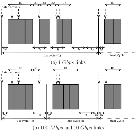
Cycle analysis. The behavior of 1000Base-T EEE links over time can be seen in

Fig. 3.1a. The figure shows a whole cycle starting with the arrival of a batch that causes the transition from state LPI to state A, continuing with an exchange between busyBi and incomplete periods S and ending after a complete period S of durationTS followed by an

period LPI.

For 100Base-Tx and 10GBase-T EEE links the behavior is different since after the link enters in state S, it cannot immediately exit but after completing both states S and W, as can be seen in 3.1b. The total length of the cycle is defined byTC and its average value is given byE[TC].

To compute the total power consumption of the system model all we need to do is to find the utilization factor of each state, and multiply it by the power consumption of the corresponding state. To do that we will use results from the renewal theory and we will estimate the average time spent in each state during a cycle over the average cycle duration. The utilization factor is denoted asρα whereα defines the four possible states of the link

(A, S , W and LPI). Thus the total power consumption of the proposed model is given by:

Ptotal=ρAPA+ρSPS+ρWPW +ρLP IPLP I,with

X

α

ρα = 1 (3.1)

Reviriego et al [9] prove thatPA≃PS ≃PW and therefore Eq. 3.1 is transformed to:

Ptotal= (1−ρLP I)PA+ρLP IPLP I (3.2)

Next, we want to derive the cycle parameters for the two cases of (1) 100M bpsand

10 Gbps EEE link and (2) 1 Gbps EEE links. Exceptionally, even though the standard specifies that1GbpsEEE links can go to state LPI only when there is no traffic in both link

(11)

7 Chapter 3. Analytical Model

(a)1_Gbps_links

(b)100_{M bps}_and10_Gbps_links

Figure 3.1: System cycle for EEE links.

directions, we assume unidirectional link behavior for the following reasons. First, earlier measurements [10] have shown that it is a good approximation to use unidirectional traffic and that the superposition of the traffic in the two link directions can model with acceptable deviation bidirectional links when the load in one direction is very low or the loads in the two directions are strongly asymmetric. Second, the correlation of traffic in the two link directions is difficult to model. Indeed, there are no models available in the literature that consider bidirectional traffic on1GbpsEEE links.

3.1

1

Gbps

Unidirectional EEE Links

To find the utilization factors we first need to compute the time that the link stays in each state. Fig. 3.1a shows the different state transitions of the link during a whole cycle over time. The analysis in based on [10].

IntervalTW. The wake-up interval has a fixed duration ofTW. IntervalTS. The sleep interval has a fixed duration ofTS.

Interval TLP I. State LPI state lasts until the first batch arrival in the interface. Since

arrival processes are Poisson with rateλits average is:

E[TLP I] =

1

λ. (3.3)

IntervalB0. B0 denotes the state A after the link has exited from the state LPI. In an M/G/1 queue with batch arrivals and arrival rate λthe average duration of a busy period is given by the number of batches received (one batch that caused the transition to state A and the batches received during TW), the mean service rate of a batch E[Sp]E[Nb]/R

(12)

8 Chapter 3. Analytical Model

ρ= _RλE[Sp]E[Nb]. Thus [12],

E[B0] = (1 +λTW)E[Sp]E[Nb]

R(1−ρ) (3.4)

IntervalBi, fori >0. Bi denotes state A after the link has exited without completing

state S (intervalsB1, B2 etc. in Figs. 3.1a, 3.1b). This expression is similar to Eq. 3.4 with

the difference that there is not the intervalTS.

E[Bi] = E[Sp]E[Nb]

R(1−ρ) ,∀i >0. (3.5)

Interval X. When the sleeping timeTS is not completed due to an arrival, there is an

interval X between the end of a busy period and the beginning of the next busy period. Otherwise, there is noX interval at all. X is then a random variable with truncated expo-nential distribution and rateλ. Therefore, its distribution is as follows:

fX(t) = λ1e

−λt

1−e−λTS, t∈[0, TS]. (3.6)

Accordingly, the average ofXis as follows:

E[X] = 1

λ−

Ts

eλ TS ₋₁. (3.7)

Number of repetitions N. Busy intervals Bi, i ≥ 1,occur if the residual interarrival time at the end of the previous busy interval is shorter thanTS. We call this residual inter-arrival intervalX. Since arrivals are Poisson, the probability of having no arrivals inTS is

P0 = e−λ TS_{. Thereby, the number}N _≥ 0_{of busy periods of type}Bi _{in a cycle, i.e., not}

counting B0, can be seen as the number of consecutive successes of a geometric random variableN with success probability1−P0. Hence, its average value is:

E[N] = 1−P0

P0 =e

λ TS ₋₁_. _(3.8)

Theorem 1. In unidirectional 1000Base-T EEE links the average cycle duration is given by:

E[T_C′ ] =TW +TS+E[N]·E[X] +E[B0] +E[B1] +

1

λ; (3.9)

orE[T_C′] = λTW +e

λTS

λ(1−ρ) . (3.10)

Proof. By summing up all the previous intervals the proof follows.

Therefore,

(13)

9 Chapter 3. Analytical Model

ρ′_A= E[B0] +E[N]E[Bi]

E[T′

C]

; (3.11)

ρ′_L= 1

λE[T′

C]

; (3.12)

ρ′S =

eλTS−1

E[T′

C]

; (3.13)

ρ′_W = TW

E[T′

C]

. (3.14)

3.2

100

M bps

and

10

Gbps

Unidirectional EEE Links

The utilization factors for these two cases can be found by following the same procedure as previously. The difference is that in case that a packet arrives in state S, it has to wait for state S to complete and for the link to wake up (TW). In Fig. 3.1b we can see the state transitions of100M bpsand10Gbpslinks during a whole cycle over time. We observe that for similar traffic the behavior of the links is different compared with1 Gbpslinks. Thus, the intervalBi(fori >0) lasts for:

E[Bi] =

(1 +λ(TS+TW −E[X]))E[Sp]E[Nb]

R(1−ρ) ,∀i >0; (3.15)

where intervalXdenotes the elapsed time before the arrival of the first packet in state S. Some analytical results from Sec. 3.1 can be reused here. I.e., E[B0]is the same as in Eq. 3.4,E[N]is like in Eq. 3.8 andE[X]is the same as in Eq. 3.7, the result for the average cycle time is given by the next Theorem:

Theorem 2. In unidirectional 100Base-T and 10GBase-T EEE links the average cycle du-ration is given by:

E[T_C′′] =TW +TS+E[N]·(TW +TS+E[Bi]) +E[B0] + 1

λ; (3.16)

orE[T_C′′] = 1 +λ(TS+TW)e

λTS

λ(1−ρ) . (3.17)

Therefore,

(14)

10 Chapter 3. Analytical Model

ρ′′_A= E[B0] +E[N]E[Bi]

E[T′′

C]

; (3.18)

ρ′′_L= 1

λE[T′′

C]

; (3.19)

ρ′′S =

TS+E[N]TS E[T′′

C]

= e

λTS_TS

E[T′′

C]

; (3.20)

ρ′′_W = TW +E[N]TW

E[T′′

C]

= e

λTS_T

W E[T′′

C]

. (3.21)

3.3

Deriving Model Parameters from Measurements

Results reported in Sections 3.1 and 3.2 show that the model requires the knowledge of some parameters. However, parameters TS, TW andR are determined by the Ethernet

link speed, whileρ, λ, Nb andSp depend on the traffic. These parameters can be given as arbitrary input to the model, as well as estimated from real traces.

E[Sp]andρcan be directly estimated from a trace. For the rest, all we need to do is to

compute the first two moments of the packet interarrival time, namely the averageE[Y]and the varianceV[Y]. In fact, assuming that batches are exponentially distributed with success parameterpbwe have that:

E[Nb] =

1 1−pb

. (3.22)

Then letY be the interarrival time between packets. Since we consider arrival in batches, the average interarrival time between packetsE[Y]is given by:

E[Y] = 0·pb+ 1

λ·(1−pb) =

1−pb

λ ; (3.23)

where in Eq. 3.23 the first term is the delay that packets suffer within the same batch (virtu-ally zero delay) times the success probabilitypband the second term is the delay that packets suffer due to the next batch, times the probability of success in this case (1-pb).

Similarly, the variance is given by the next formula:

V[Y] =

q

1−p2 b

λ . (3.24)

Solving Eq. 3.23 and Eq. 3.24 we can findλandpb and then we can also computeE[Nb].

With the above, all parameters are computed. Therefore, we remark that using the model for real traffic traces only requires to estimate from the trace the following basic parameters:

(15)

Chapter 4

Energy Efficiency in Web Hosting

Centers

In this section, we summarize the results of our measurement campaign conducted in collaboration between Institute IMDEA Networks and InterHost. With our measurements, we have characterized the behavior of the aggregate traffic flowing through one of the Inter-Host’s firewalls at one of their web hosting centers located in Madrid, Spain. We have used the collected data in order to evaluate the potential for power saving that could be achieved by replacing the company’s gigabit wired links with EEE connections. Furthermore, we plot the daily load and the potential power savings computed by simulating the measured traffic with a C++ EEE link simulator, and using the model that we previously explained in Chapter 3 for predicting the EEE and it is further analyzed in [10].

4.1

Motivation

The goal of our measurement is to collect enough data to characterize the traffic behavior of a real commercial installation, and to provide an estimate of the power saving that might be achieved at the data center by replacing existing Ethernet links with IEEE 802.3az energy saving Ethernet links. We need these traffic measurements to compute the first two moments of the packet interarrival rate, the average packet size and the offered link load, and use these parameters to feed the EEE model that we previously analyzed in Chapter 3. As explained in Chapter 3, the model in Chapter 3 is able to predict the average time spent by an EEE link in state LPI, thus allowing to estimate the amount of power saving that can be achieved with a given input traffic pattern, when EEE links are adopted.

The model does not consider that, for 1000Base-Tx links, the IEEE802.3az standard specifies that the link can go to low power state only when no traffic is present in both link directions. So the model ignores the correlation of traffic flows in the two link transmission directions. However, results shown in [10] demonstrate that that model can be suitably used to predict the power saving of EEE 1000Base-Tx links when the link is strongly asymmetri-cally loaded in the two transmission directions, and when the less loaded direction works at few percents of its capacity. To achieve such prediction, it is enough to consider the traffic in the most loaded link direction only (cf. Table II in [10]).

(16)

12 Chapter 4. Energy Efficiency in Web Hosting Centers

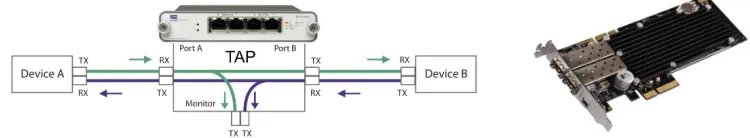
(a) Measurement architecture and TAP device (image from NetOp-tics website).

(b) The Endace DAG card (image from Endace website).

Figure 4.1: Measurement tools.

Here we want to test our model’s performances under a broader range of realistic traffic matrices, and we want to take into account the correlation of traffic flows in the two link directions. Obtaining real data is usually very difficult, so that synthetic traffic generator is the obvious, though less accurate, alternative. In our case, InterHost allowed us to monitor the traffic at the interface between Internet and one of InterHost’s firewalls. This gives us the advantage of using real data and real traffic that yields more realistic results. However, in respect of user’s and company’s privacy and security, we only capture few bytes of each packet, and we do not inspect the payload. Actually, our goal is to capture the arrival time of the packet and its size, which is enough for our purposes.

To achieve our goal, we need to collect precise and clock-synchronized timestamps for packet arrivals over the two link directions. Therefore we need precise measurement tools and a measurable source of real traffic.

In this rest of this Section we show that a huge amount of power might be saved at InterHost by replacing the legacy Ethernet links with EEE links, the power saving being a periodic function of the time of the day and the day of the week. More than 40% of the power might be saved most of the time, with peaks of 90% or more during the night hours. We also show that noisy measurements might severely impact the quality of our EEE power saving estimate as soon as the maximum timestamp deviation due to noise reaches a few millisec-onds, which is below the typical timestamp accuracy of non-dedicated network hardware, i.e., of inexpensive but imprecise driver time-stamping. This justifies using specialized high accuracy time-stamping hardware.

4.2

Unintrusive Measurements at InterHost

All we need for our EEE power saving estimate is to compute the first two moments of the packet interarrival time, the average packet size, and the offered load. However, we can also simulate the EEE operation by using real traffic traces as an input arrival process [10]. With the simulator we can compute the exact EEE power saving, and compare this value with the estimate yielded by the model. The simulator needs an input trace file containing, for each packet, the timestamp of the packet’s arrival time, and the size of the packet. Therefore, we do not need to parse the content of any packet, and there is no need to save the content of each packet for post-processing. All we need is an accurate sniffer, whose architecture is described in what follows.

(17)

du-13 Chapter 4. Energy Efficiency in Web Hosting Centers

plicate real packets without affecting the traffic. The tap is shown in Figure 4.1a. We use a NetOptics passive device which is inserted in a 1000Base-TX Ethernet link and dupli-cates each and every signal over the link.1 The NetOptics device, as shown in the figure, is also able to separate the traffic in the two directions, i.e., it provides the traffic in the two directions over two separate cables to be connected to a monitor device.

We use a Linux Dell Xeon server with1T byteof memory to store the monitored data. The two monitoring ports of the tap are connected to a digital capture card, specifically a high accuracy two-port Endace DAG card as the one shown in Fig. 4.1b.2 The DAG card is a dedicated capture device with dedicated CPU and memory, able to capture 100% of the traffic at up to10 Gbpsover each direction. Furthermore, the DAG card has a unique time-stamping engine that guarantees clock synchronization to the nanosecond over the two monitoring ports.

The tap is placed within the link that we want to measure, i.e., in front of one of Inter-Host’s firewalls, and the DAG is activated once per hour to collect at most 100 bytes per packet for 200 seconds. The link speed is1Gbps.

We keep as well a remote ssh connection with the server, so that we can periodically transfer the collected traces to a Linux server located in our lab at Institute IMDEA Net-works. Once the traces are in our lab, we post-process them with the tshark packet analyzer and create simplified and anonymous trace files containing only the timestamp of each packet arrival and its size in bytes.

4.3

Using the Collected Traces (EEE Simulation and Model)

We have been capturing traffic traces from November 26, 2011 to the present days (end of August 2012). Therefore, we now have enough data to characterize the traffic behavior over the measured InterHost’s link. In particular, we observe a daily typical maximum traffic of about 4-5% in the most loaded link direction, with the exceptional value of 11% on one traffic direction on February 8, 2012.

After collecting a trace, we post-process the captured packet fragments to generate a simple two-column file containing a timestamp and a packet size for each link transmission direction. Once the simplified traces are ready, we first simulate the EEE operation with an ad-hoc developed C++ simulator [10], then we extract the statistical parameters needed to run the EEE model and estimate the EEE power saving though the model discussed in Chapter 3 as well.

In the following subsections we show our measurements together with the EEE power saving as computed via the simulator in each of the sampled traffic intervals. Model results will be compared to the simulation in Section 4.6.

4.4

Traffic Behavior and EEE Power Saving

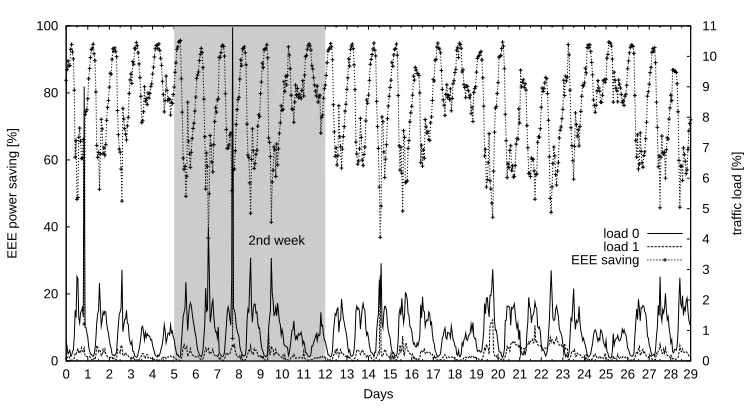
In Fig. 4.2 we plot the monthly load in each direction for February 2012, which is rep-resentative of our measurements and the power saving that might be achieved by means of

1

http://www.netoptics.com/products/network-taps

(18)

14 Chapter 4. Energy Efficiency in Web Hosting Centers

0 20 40 60 80 100

0 1 2 3 4 5 6 7 8 9 10 11 12 13 14 15 16 17 18 19 20 21 22 23 24 25 26 27 28 29

0 1 2 3 4 5 6 7 8 9 10 11

EEE power saving [%]

traffic load [%]

Days

2nd week load 0_{load 1}

EEE saving

Figure 4.2: The power savings during a whole month.

EEE links. Our observations are that we have a maximum traffic load of about 5% in the most loaded direction, but for holidays and weekends, when the peak load is below 2%. In the figure, traffic patterns are quite regular, showing higher traffic activity over 5 consecutive days (corresponding to the Monday-Friday period), followed by low traffic intensity over the weekend It is also evident that overnight the traffic is very low.

Processing the collected data with the EEE simulator reveals that overnight and during the weekend, EEE might save 70-90% of the power with respect to legacy Ethernet. Even during weekdays the power saving might be at least about 40% during the peak hours.

Considering that a gigabit Network Interface Card (NIC) consumes about 2 W (e.g., see Intel 1G datasheets [13]), the estimated power saving for a single link with two NICs connected sums up to 1.1 to 2.6 KW h/month, these numbers being relevant for large data centers or web hosting companies running tens of thousands of links. For example, consider a typical large data center (more than 4650 m2

nowadays [14]) with ∼40,000

servers (like Google’s data centers [15]). According to [16] each server has three network ports on average. Therefore, in total, the data center runs about 120,000 network ports, each of which will typically be very low loaded. Thereby, the power saving could be close to the peak most of the time. Considering the average price of electricity in Europe, i.e.,

∼ 0.15Euros/KW h, using EEE links might generate a potential economy of more than

280,000Euros/year. The case of10Gbps(and100Gbps) links is even more promising,

since they consume even more power, i.e.,4.5−20W according to [13].

4.5

Zooming over the Weekly Saving

(19)

15 Chapter 4. Energy Efficiency in Web Hosting Centers 0 20 40 60 80 100

0 1 2 3 4 5 6 7

0 2 4 6 8 10 12

traffic load [%]

Days

Weekly plot from January 30th until February 5th (1st week)

(Weekend)

load 0 load 1 EEE saving

(a) Power saving during the first week of February.

0 20 40 60 80 100

0 1 2 3 4 5 6 7

0 2 4 6 8 10 12

traffic load [%]

Days

Weekly plot from February 6th until February 12th (2nd week)

(Weekend)

(b) Power saving during the second week of February.

0 20 40 60 80 100

0 1 2 3 4 5 6 7 0

2 4 6 8 10 12

traffic load [%]

Days

Weekly plot from February 13th until February 19th (3rd week)

(Weekend)

(c) Power saving during the third week of February.

0 20 40 60 80 100

0 1 2 3 4 5 6 7 0

2 4 6 8 10 12

traffic load [%]

Days

Weekly plot from February 20th until February 26th (4th week)

(Weekend)

(d) Power saving during the forth week of February.

Figure 4.3: Weekly plots.

traffic distribution over time clearly depends also on the nature of the websites hosted at InterHost premises, about which we have no information. However, the measured traffic patterns are qualitatively in line with other traffic patterns reported in literature.

4.6

Impact of Noisy Measurements

(20)

16 Chapter 4. Energy Efficiency in Web Hosting Centers 0 2 4 6 8 10 12

0 1 2 3 4 5 6 7 8 9 10 11 12 13 14 15 16 17 18 19 20 21 22 23

Power savings [%]

time [hours] Load in each direction Load 1

Load 2

(a) Load in each link direction.

0 10 20 30 40 50 60 70 80 90 100

0 1 2 3 4 5 6 7 8 9 10 11 12 13 14 15 16 17 18 19 20 21 22 23

Power savings [%]

time [hours]

EEE savings on Feb 8th, 2012, with uniformly distributed noise in [- 5, 5] µs

Simulation (w/out noise) Simulation (w/ noise) Model (w/out noise) Model (w/ noise) Model (Load 1 w/out noise) Model (Load 1 w/ noise)

(b) Noise within±_{5 microseconds.}

0 10 20 30 40 50 60 70 80 90 100

0 1 2 3 4 5 6 7 8 9 10 11 12 13 14 15 16 17 18 19 20 21 22 23

Power savings [%]

time [hours]

(c) Noise within±_{50 microseconds.}

0 10 20 30 40 50 60 70 80 90 100

0 1 2 3 4 5 6 7 8 9 10 11 12 13 14 15 16 17 18 19 20 21 22 23

Power savings [%]

time [hours]

(d) Noise within±_{500 microseconds.}

0 10 20 30 40 50 60 70 80 90 100

0 1 2 3 4 5 6 7 8 9 10 11 12 13 14 15 16 17 18 19 20 21 22 23

Power savings [%]

time [hours]

(e) Noise within±_{5 milliseconds.}

0 10 20 30 40 50 60 70 80 90 100

0 1 2 3 4 5 6 7 8 9 10 11 12 13 14 15 16 17 18 19 20 21 22 23

Power savings [%]

time [hours]

(f) Noise within±_{50 milliseconds.}

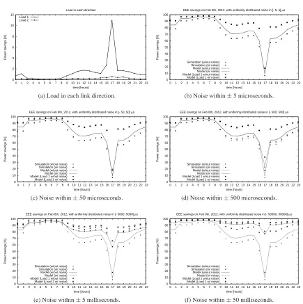
Figure 4.4: Noise introduction.

over the aggregate traffic measured over the two link directions, we merge the traffic traces obtained for the two directions. As a consequence, the model cannot completely capture the correlation of traffic in the two directions. In fact, the IEEE 802.3az standard says that link interfaces can enter the low power state only when both link directions are idle. Instead, we are simplifying the model to cope with a unique link direction, possibly resulting from the merging of the two real link directions.

(21)

17 Chapter 4. Energy Efficiency in Web Hosting Centers

registered over the daily samples is depicted in Fig. 4.4a, and it achieves a maximum value of 11% over the most loaded link direction. That load is not affected by our timestamp alterations.

The extremes of the added noise span from±5 microseconds in Fig. 4.4b and go up to

±50 milliseconds in Fig. 4.4f. Each plot contains two lines that indicate the power saving estimates obtained with the model computed on the aggregate link traffic (merging of the two traffic directions), with and without the artificially added noise. The figures also report the EEE power saving as estimated by the model when considering only the traffic in the most loaded link direction (which is Load1 in the figures), with and without timestamping noise. Finally, the figures include the EEE computed through the simulations, with and without noise. Therefore, in each plot, the values obtained without noise are always the same, thus representing the benchmark for these experiments.

From the figures, we note that model and simulator report similar trends, with close but distinct power saving estimates. Differences are well explained considering that the model does not capture the bidirectional nature of the EEE power saving mechanism. Limited differences are due to the low load measured on both link directions. The model which only consider the most loaded link is obviously the one reporting the highest power saving. Similarly, the model considering the aggregate traffic yields the lower power saving, since it does not consider that packets belonging to opposite traffic directions might be served in parallel.

Let’s now consider the impact of noise. As we can see in Figs. 4.4b to 4.4f, with the introduction of noise in the order of up to one millisecond, the curves obtained with and without noise almost overlap. In contrast, with the introduction of more noise, we can see that the graphs obtained with noisy measurements tend to achieve higher power saving. In fact, adding noise to timestamps contributes to break the traffic correlation between the two directions, so that(i)simulator and model yield very similar results, and(ii)power saving occurs with roughly the product of probabilities of having each link direction idle. As a result, about 80% power saving can be erroneously estimated even for the peak hour.

(22)

Chapter 5

Related Proposals

A few number of similar works on EEE appeared recently in the literature. In the fol-lowing subsections, we first present the related analytical model in [10], second we show the results of existing evaluations on EEE links based on [4, 9] and last we introduce enhance-ments for future EEE systems that might boost the performance of EEE in terms of power saving [18, 19].

5.1

Evaluation of EEE

5.1.1 Model

In [10], Ajmone Marsan et al. model the behavior of EEE links with independent traffic in the two link directions, and validate their model by means of real traces for1Gbpsand

10Gbpslinks. The authors describe the behavior of EEE links in a similar manner as we also did in this thesis. Additionally, using a simulator that was developed by the authors, they predict the power saving of real traces with EEE links instead of the legacy Ethernet. They make use of traces obtained by Google’s data centers and CAIDA [20, 21]. The final simulation results are very close to the ones from the model. However, they evaluate10Gbps

EEE links using CAIDA traces for backbone links, so that their results cannot be used for data centers using1Gbpslinks. Similarly, the number of1Gbpstraces considered in that paper is limited to a few units so that their results cannot be easily generalized to broader scenarios. Moreover bidirectional Google datacenter traces are not synchronized with high precision since the authors could not access the data center and use high precision tools.

5.1.2 Simulation Results

In [4] the authors first simulate the behavior of EEE links and then estimate the power consumption of different scenarios by capturing real traces.

The simulations were realized for three different link speeds: (1) 100 Base −T x,

(2) 1000 Base−T and(3) 10 GBase−T. For every example case it is assumed that each link direction is independent of the other and so the link is allowed to be, e.g., in state LPI in one direction and in state A in the other direction. Like we previously said this is not the case for 1000Base-T links, but for simplicity and similarly to what we did in Chapter 3,

(23)

19 Chapter 5. Related Proposals 0 20 40 60 80 100

0 0.2 0.4 0.6 0.8 1

Power Consumption [%]

Load 100 Mbps links

energy proportionality with EEE without EEE (a) 100Base-T 0 20 40 60 80 100

0 0.2 0.4 0.6 0.8 1

Load 1000 Mbps links

energy proportionality EEE without EEE (b) 1000Base-T 0 20 40 60 80 100

0 0.2 0.4 0.6 0.8 1

Load 10 Gbps links

energy proportionality EEE without EEE

(c) 10GBase-T

Figure 5.1: Power consumption vs. Load (data from [4]).

the authors of [4] use the unidirectional behavior assumption also for1GbpsEEE links. In their paper is further assumed that large frames of10000bitsare exchanged and they arrive according to Poisson distribution. This identifies the best case for EEE links since, com-paring the transmission time of such highly aggregated traffic with the intervalTS+TW, we observe that the overhead produced is less significant. In fast networks, if we only send small packets (e.g., acknowledgments) the power overhead could be huge sinceTf rame(the

time needed to transmit a frame) is relatively small compared withTS+TW. Last

assump-tion in [4] is that state LPI consumes about 10% the power of state A. Simulaassump-tions proposed in [4] are compared on one side with the ideal case of energy proportionality [17], where power consumption is given by the formula:

Pideal =PActive·Load+PLP I·(1−Load); (5.1)

and on the other side with the case of legacy power-unaware Ethernet links. The results of the simulations are illustrated in Fig. 5.1. We can observe that, for100M bpslinks, energy consumption is more energy proportional than it is for1000M bpsand10Gbpslinks. This is because the overhead in time due to state S and W is very large compared with the data transmission inGbpslinks.

(24)

20 Chapter 5. Related Proposals

behavior. These are:

• A user who is connected to its ADSL router using100M bpsconnection and down-loads some video files.

• Two users are connected between each other using 100 M bpsLAN connection to exchange a file.

• A university access link of1000M bpswith highly multiplexed Internet traffic.

• Some traces from Google’s data centers.

The first scenario is typical for residential users with ADSL connection from 1M bps

to10M bpswhere the load between the router and the user is very low. Nowadays, newer

Ethernet cards with link speeds of1 Gbpsor more between the router and the user result in lesser load. In the second scenario the authors generate heavy traffic for the link in one direction (continuous traffic), while in the other direction only “ACKs” are transmitted and the link is very low loaded. The third scenario has a medium traffic of about 10-17% in each direction. In the last scenario various traces from Google’ s data centers have agnostically been used.

Except from the first scenario where the links save about 90% of energy, the rest of the scenarios perform very poorly in terms of energy consumption. We can see in [4] that when the frame size reaches its maximum value (1500 Bytes) the power consumed is propor-tional to the traffic, while for medium and small packet sizes the power consumption of EEE approaches 100%, i.e., same as legacy Ethernet links.

5.1.3 Performance Measurements of Real Cards

In [9], the authors realize measurements in NIC cards and they observe their power consumption behavior.

The experiments are made using two NIC cards with integrated EEE functionality. Since the measurements are based on the power consumed by the NIC cards, this power represents both PHY and MAC layers plus the PCIe interface and the integrated voltage regulator of the card. Accordingly, the expected results show less power saving (in percentage) than expected, since these elements (MAC and PCIe interfaces) do not benefit from EEE. Initially, different length of cables were used, to test if this factor influences the power consumption of the card but since there was only a small variation of about 2%, a fixed cable length was used for other experiments. Last but not least, the highest supported speed by the cards was mostly used for the experiments, that is1000M bps, while in some of them100M bpsspeed was used for reference reasons.

Three scenarios were tested.

• The power consumption of the link in the case of no traffic versus a heavy loaded link.

• The power consumption of the link during state transitions.

(25)

21 Chapter 5. Related Proposals

In the first scenario, the two NICs exchange a video file (continuous traffic of big pack-ets) and the authors measure the power consumption with and without EEE. A reduction of about 70% is observed for1000M bpslinks and about 30% for100M bpslinks. The power saving is not as high as expected because the additional components of the NIC card do not benefit from the use of EEE as we previously said. Additionally, since we use the same card for both link speeds the energy overhead produced by these components is more dominant for the low speed than for the high speed.

In the second scenario, scarce traffic (which produces frequent state transitions) is gen-erated to challenge the link at both speeds. More specifically, small packets of250bytesare used with a data rate of10M bpsso the packets arrive almost equally spaced everyTS+TW

and the link is either in state A or in one of the transition states. The power consumption for this case is similar to the power unaware schemes. So, we understand that the power consumption of transition states is similar to the power consumption of the state A.

In the last scenario the video file is again exchanged for various data rates over

1000M bpslinks. Two observations were made. First, when the link load is over 6% there

is no power saving, because we have a huge energy overhead due to continuous EEE state transitions. Second, we observe that the link is active in both directions because we have high data traffic in one direction and we receive scarce ACKs traffic in the other direction.

5.2

Boosting Energy Efficiency with Packet Coalescing

The previous evaluations shows that EEE behaves quite well when there is scarce traffic on the links and when large packets of1500bytesare transmitted over the network, like for video files. However, when there is heavier traffic (e.g., load > 15%) then EEE behaves similar to power-unaware schemes. This is because of the overhead produced by the state transitions of the links. For instance, with a traffic pattern of small packets (100−200bytes) equally spaced between them (every 150-200µs), a1000M bpslink will spend 95% of the time in EEE state transitions. So, since the idea of a “low power” state is brilliant and this is the method that is usually suggested in order to reduce the power consumption of a device (e.g., base stations, mobile devices, monitors, laptops, smart phones, televisions), further enhancements towards this direction are needed to achieve the initial goal for power reduction even when traffic is not very low and/or packet sizes are small. As we previously said, one possible policy going in this direction is the hardware optimization using more efficient electronics to transit faster (open research area for hardware producers) and a second possible policy is the use of efficient algorithms to handle both the packets and the link and remain for greater time in state LPI.

In this section we shortly investigate on the second policy, namely packet coalescing, and we show an efficient algorithm to reshape traffic and handle packet more efficiently in terms of power. Initial studies have been realized in [18, 19]. The basic idea is as follows: when there are no packets to transmit switch to state LPI, then store the new arriving packets in a buffer and wait until the buffer fulls or a timer expires. Then switch to state A and transmit. Next, we get into more details about how this policy works.

(26)

22 Chapter 5. Related Proposals 0 20 40 60 80 100

0 0.2 0.4 0.6 0.8 1

Energy Consumption [%]

Load Energy vs. Link Load

energy proportionality EEE legacy coalesce 10pkts coalesce 100pkts

(a) Power Consumption with coalescing.

0 20 40 60 80 100

0 0.2 0.4 0.6 0.8 1

Delay/packet

µ

s

Load Added delay using coalescing w/o EEE

EEE Scenario 2 Scenario 1

(b) Delay of packets using various coalescing sizes.

Figure 5.2: Impact of coalescing on power save and on delay (data from [18]).

less power. For implementing coalescing we need two things.

• A coalescing buffer to collect and store the packets. Simulation results in [18, 19] show that depending on the size of packet coalescing, EEE can obtain results very close to the energy proportionality. The bigger the buffer size the more the power saving as we see in Fig. 5.2a. Indeed, Fig. 5.2a illustrates that a burst of ten packets reduces the power consumption by half than EEE without a coalescer. With a burst of hundred packets we see that the power consumption approaches the ideal case (data from [18]).

• A timerTcoalescecan trigger the buffer interface to start sending packets and empty the coalescing buffer in cases of low traffic, to avoid waiting for hours in case of scarce traffic, e.g., a few “ACKs”. So, either the buffer fulls and we start sending the packets together with the ones that arrive, or we wait until the timer expires.

However, there are two main drawbacks due to coalescing. First, the added delay to the packets can reach at leastTcoalesce+TW for the worst case and second, sending bursts of packets to the network where in the worst case they are as big as the buffer size is not a desirable property for IP networks. In fact, bursts will flood the network and may cause buffer overflows to intermediate routers. Both of these drawbacks degrade the network per-formance.

(27)

Chapter 6

Conclusions

Until recently, there were not many enhancements in the network core in terms of energy efficiency. Higher network speeds, bigger capacity, fast routing are the results of an in-creased demand of network services such as video files, movies, online TV, etc. Network companies deployed a lot of kilometers of copper and fiber together with routers and servers and a lot of new Ethernet ports especially in developing countries to satisfy the customers and adapt to their needs. Furthermore, higher Ethernet speeds require more power to operate properly since they have more complex electronics in order to meet the standards. This led to an increased power consumption. Thus, a new Ethernet standard was proposed by IEEE, to deal with energy efficiency, namely Energy Efficient Ethernet-EEE (IEEE 802.3az).

The idea behind EEE is simple. Four new states are introduced, “Active”, “Low Power Idle” (LPI), “Sleep” and “Wake Up”. When there is data to send over the Ethernet link the link operates as usual in “Active” state but when there is no data to send, it transits to LPI state, consuming only 10% of the initial power. The transition time between “Active” and LPI state defined as the “Sleep” state and the transition time between LPI and “Active” state defined as the “Wake Up” state.

A priori, this method looks fine when the traffic is scarce (<15%) and long intervals exist between the packets. In contrast, in cases where traffic is heavy and short intervals separate the packets, EEE may not provide significant improvement since it has a lot of power overhead due to state transitions. Therefore, in this thesis, we studied the power save in real scenarios and reported on novel proposals aiming at enhancing EEE performance when traffic is not scarce and spacing among packets is short. The main goal of our work was to collect and analyze unique data on bidirectional traffic in a real network, and estimate the potential savings that can be achieved by adopting the recently released IEEE Standard 802.3az instead of the legacy Ethernet. Overall, we observed traffic patterns yielding the possibility to save at least 40%, and up to more than 90%, in each gigabit link. Such a power saving would represent a non-negligible operational cost reduction for a data center, in the order of several hundreds of thousands of Euros per year. Moreover, we analyzed the importance of high precision traffic measurements on the power saving estimation. Our analysis unveils that precise timestamping is needed to use analytical models, which allows EEE power saving estimation with no need for time consuming simulations.

Another goal of our work was to describe various techniques that have been proposed to reduce the power consumption of EEE even in cases of high traffic or short spacing among

(28)

24 Chapter 6. Conclusions

(29)

References

[1] European Commission (DG INFSO), Study of the impacts of ICT on energy efficiency, 2007

[2] C. Gunaratne, K. Christensen, B. Nordman, S. Suen, Reducing the energy consumption

in Ethernet with Adaptive Link Rate(ALR), IEEE Trans. Computers, vol. 57, no. 4, pp.

448-461, 2008.

[3] IEEE Std 802.3az: Energy Efficient Ethernet-2010.

[4] P. Reviriego, J.A. Hernandez, D. Larrabeiti, J.A. Maestro, Performance Evaluation of

Energy Efficient Ethernet, IEEE Communication letters, vol. 13, no.9, pp. 697-699, Sep.

2009.

[5] R. Sohan, A. Rice, A.W. Moore, Characterizing 10 Gbps Network Interface Energy

Consumption, 35th IEEE Conference on Local Computer Networks, Oct. 2010.

[6] M. Gupta, S. Grover, S. Singh, A feasibility study for power management in LAN

Switches, IEEE International Conference on Network Protocols, pp.1092-1648, 2004.

[7] B. Nordman, EEE savings estimate, IEEE 802.03az Task Force Information, Mar. 2008.

[8] V. Mancuso, A. Chatzipapas, On IEEE 802.3az Energy Efficiency in Web Hosting

Cen-ters, to appear in IEEE Communication LetCen-ters, 2012.

[9] P. Reviriego, K. Christensen, J. Rabanillo, J.A. Maestro, An Initial Evaluation of Energy

Efficient Ethernet, IEEE Communication letters, No. 5, Vol. 15, May 2011.

[10] M. Ajmone Marsan, A. Fernandez Anta, V. Mancuso, B. Rengarajan, P. Reviriego Vasallo, G. Rizzo, A Simple Analytical Model for Energy Efficient Ethernet, IEEE Com-munication letters, No. 99, pp. 1-3, June 2011.

[11] R. Jain, S. Routhier, Packet trains-Measurement and a New Model for Computer

Net-work Traffic, IEEE Journal of Selected Areas in Communications, vol.4, no.6,

pp.986-995, Sep. 1986.

[12] L. Kleinrock,Queueing Systems, volume 1: Theory, Wiley 1975.

[13] R. Sohan, A. Rice, A.W. Moore, K. Mansley, Characterizing 10 Gbps Network

Inter-face Energy Consumption, in 35th IEEE Conference on Local Computer Networks, Oct.

2010.

(30)

26 REFERENCES

[14] S. Bapat, The Future of Data Centers (... and the Stuff That Goes In Them), http://www.e3s-center.org/events/09/e3s-symposium.htm, June 2009.

[15] Google, Google Data Center Video Tour, http://www.google.com/about/datacenters/events/2009-summit.html#tab0=4, Apr. 2009.

[16] U.S. Environmental Protection Agency, Energy Star Program, Report to Congress on

Server and Data Center Energy Efficiency, Public Law 109-431, Aug. 2007.

[17] L.A. Barroso, U. Holze, The case for energy-proportional computing, IEEE Computer, vol. 40, no. 12, pp. 33-37, Dec.2007.

[18] K. Christensen, P. Reviriego, B. Nordman, M. Bennett, M. Mostowfi, J.A. Maestro,

IEEE 802.3az: The Road to Energy Efficient Ethernet, IEEE Communications

Maga-zine. Vol.48, no.11, pp.50-56, Nov. 2010.

[19] P. Reviriego, J.A. Maestro, J.A. Hernández, D. Larrabeiti, Burst Transmission for

Energy Efficient Ethernet, IEEE Internet Computing, Jul. 2010.

[20] C. Walsworth, E. Aben, K.C. Claffy, D. Andersen, The CAIDA anonymized 2009

In-ternet Traces, http://www.caida.org/data/passive/passive_2009_dataset.xml.