User Association to Optimize Flow Level Performance in Wireless
Systems with Dynamic Interference
?
Balaji Rengarajan and Gustavo de Veciana 1 IMDEA Networks{[email protected]} 2 University of Texas at Austin{[email protected]}
Abstract. We study the impact of user association policies on flow-level performance in interference limited wireless networks. Most research in this area has used static interference models (neighboring base stations are always active) and resorted to intuitive objectives such as load balancing. In this paper, we show that this can be counterproductive in the presence of dynamic interference which couples the transmission rates to users at various base stations. We propose a methodology to optimize the performance of a class of coupled systems, and apply it to study the user association problem. We show that by properly inducing load asymmetries, substantial performance gains can be achieved relative to a load balancing policy (e.g., 15 times reduction in mean delay). Systematic simulations establish that our optimized static policy substantially outperforms various dynamic policies and that these results are robust to changes in file size distributions, channel parameters, and spatial load distributions.
Key words: User association, flow-level performance, coupled queues, semidefinite programming
1
Introduction
The high demand for wireless capacity and the increasing volume of traffic mandates the efficient use of available radio resources. Wireless capacity can be substantially enhanced by reusing the entire frequency spectrum at every transmitter instead of sacrificing individual peak and overall system capacity by partitioning it. This increased system capacity and spectral efficiency is achieved at the expense of increased interference. Even in the case of WLANs with frequency reuse, high densities of users in large scale networks could lead to high interference due to the limited number of orthogonal frequencies available under the present standards.
The bursty nature of traffic in typical wireless systems results in dynamic interference which couples perfor-mance in the system in a complex manner. For such coupled systems, stability is fairly difficult to establish, and performance is particularly hard to optimize. The capacity of such a system as well as the actual performance that users perceive can be very different from that predicted by a saturated model that assumes that transmitters are always on, see for example [1–3]. Without having access to good performance models, many researchers have resorted to intuitive objectives such as load balancing across system resources. In this paper, we show that such load balancing, be it greedily done by users or across the system, may be counter productive when there is dynamic coupling due to interference.
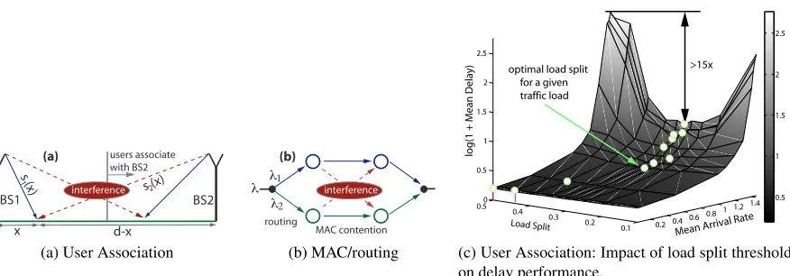
Let us consider some examples where dynamic coupling impacts network functions. Consider the user associ-ation problem exhibited in Fig. 1a. Assume that the base stassoci-ations share the same spectrum, so they interfere with each other when they are concurrently active, which in turn reduces their transmission capacity to users. For sim-plicity, assume user requests to download files arrive uniformly between base stations 1 and 2. A basic problem in such networks is to decide which base station should serve a new user request. If both the network and traffic demands aresymmetric, one might intuitively expect that a static policy that associates arrivals with the closest base station, i.e., the one that delivers the strongest signal, and thus balances the offered load, would be ‘optimal’. Surprisingly, we will see that this is not the case.
A second example is exhibited in Fig. 1b where wireless nodes relay traffic. Assume nodes contend at random for a shared channel. Depending on the amount of traffic and interference they see, one might optimize nodes’ con-tention probability for the channel so as to minimize overall packet delays. Clearly, performance here is a complex function of the dynamic traffic loads, contention probabilities, and interference seen by nodes. The third example, also shown in the same figure, concerns routing traffic across paths that are link/node disjoint. Unfortunately, trans-missions along the paths may directly (or even indirectly) interfere with each other. Should a packet flow with rate
λbe split across the two paths, or is it better to route traffic on a single path?
?This research was supported by NSF Award CNS-0917067, and Intel Research Council Grant, and performed in part under
x
BS1 BS2
users associate with BS2
(a)
d-x s (x)
1
s (x)2
interference
(a) User Association
routing
λ λ1 λ2
MAC contention
(b)
interference
(b) MAC/routing
0.2 0.40.6 0.8 1 1.2 1.4
0.1 0.2 0.3 0.4 0.50 0.5 1 1.5 2 2.5
Mean Arrival Rate
Load Split
log(1 + Mean Delay)
0.5 1 1.5 2 2.5
optimal load split for a given traffic load
>15x
(c) User Association: Impact of load split threshold on delay performance.
Fig. 1.Examples of network functions impacted by dynamic coupling
The above exemplify the relevance of dynamic coupling in optimizing network functions at various layers. In the above cases, assuming symmetry in loads and/or the network, one might imagine load balancing might be a good objective, but this need not be the case. For example, it may be preferable to route traffic on a single path so as to avoid interference across paths. In this paper, we focus on the terminal association problem which, as we will see, is already fairly complex. As mentioned earlier, when the channels and traffic load are symmetric, one might expect that associating users’ requests with the closest base station might be a good strategy. This corresponds to splitting the load evenly between the two base stations. Fig. 1c shows the simulated delay performance (explained in more detail in the sequel) when load split between the base stations is varied from 0.5 (even division of load) to 0.1 (highly asymmetric load division). The results show that the optimal load division depends on the intensity of the offered load, and is not balanced but significantly asymmetric. As exhibited in the figure, where mean delays are plotted on a logarithmic scale, the performance implications can be substantial; load balancing may achieve mean delays 15 times higher versus an optimal asymmetric split. This result is surprising, and reveals the complexity and substantial impact that dynamic coupling can have in the context of wireless networks. This motivates the need for careful analysis that we will carry out in this paper, as well as comparisons with more complex user and system greedy dynamic policies.
Related Work:Various dynamic policies that split load among base stations have been proposed for different contexts. For example, load balancing schemes have been proposed for the scenario where frequency reuse is used to protect against inter-cell interference, and where the traffic carried by the network is voice [4–6]. The objective in these works has been to ensure that load is balanced among base stations.
This philosophy has also been used in addressing the case of best effort traffic. When the wireless network is subject to spatially heterogeneous traffic loads, emphasis has been placed on the development of schemes that try to balance the load across base stations. Centralized schemes to jointly balance loads and schedule packets are presented in [7]. Such centralized schemes however, incur excessive communication and computational overhead. In [8], a load balancing scheme that requires much less coordination is considered. The scheme tries to explicitly balance the load across base stations, taking into consideration both the long term rate at which users can be served, and their load. Another idea that was proposed, also in [8], is to lower the strength of the pilot signals that heavily loaded base stations broadcast, so as to discourage users from joining them. A scheme that is similar in spirit is proposed in [9], called MAC-cell breathing, that attempts to balance the load in all base stations. The above mentioned schemes however, assume implicitly that the base stations in the network are always transmitting and thus interfering with transmissions in their neighboring cells. The focus in these schemes is to ensure that the load being served by different base stations in a neighborhood is as similar as possible.
The case of dynamic traffic, with the associated bursty interference, has not been extensively studied. In [10], the effect of equalizing the load in neighboring base stations was studied through simulation, and it was observed that load balancing did not make much of a difference under heavy load. This problem is also studied in [11], but under the assumption that transmissions are orthogonal. The impact of dynamic interference was also demonstrated in [12], wherein the problem of load balancing in a hybrid wireless local area/wide area network was studied using approximations proposed in [13].
stability region of the system is not always maximized by perfect load balancing across servers. While the above papers address the question of determining the network capacity, they do not provide insight into designing user association policies to optimize performance perceived by users in a system serving a load that is in the interior of the stability region. In contrast, the focus of this paper is on flow level performance, i.e., the actual file transfer delays experienced by users. We obtain bounds on the mean delay experienced by users in coupled systems and use these bounds to design user association policies that optimize flow level performance.
Our contributions:We study a static load allocation scheme that takes into account the long term spatial load being served by the base stations and attempts to minimize the average file transfer delay perceived by users. In addition to short-term, unpredictable variations in the load caused by individual user arrivals and departures, there are predictable long-term variations in the aggregate traffic load depending on the day-of-week, hour-of-day, etc. [16, 11]. The proposed scheme is adapted to these long-term traffic patterns, and does not depend on the instan-taneous loads or short-term variations. Such a scheme is potentially simpler than dynamic schemes which require knowledge of the instantaneous loads being served, but might be sensitive to errors in the long term traffic esti-mates. Our contributions in this context include:
1.We propose a methodology to optimize the performance of wireless systems coupled through dynamic interfer-ence and apply it to study networks with base stations distributed on a line and on a two dimensional plane. To our knowledge, prior to this work, no closed-form or good approximations were available for general systems with 3 or more coupled queues.
2.For a dynamic model of the user association problem in one dimension, we show that delay optimal static poli-cies are threshold based. Surprisingly, we find that even for a symmetric network, a policy which balances load can be highly suboptimal. Moreover, we find that asymmetric policies can improve average delays seen by users atall
spatial locations.
3.We show that an optimized static policy (asymmetric) can substantially outperform dynamic policies which are greedy from the user’s or system’s points of view and achieves performance close to that of a ‘repacking’ policy. This suggests that an important objective for protocol and network design will be to achieve such asymmetries.
4.We demonstrate through extensive simulations that the proposed policy consistently outperforms conventional, load balancing based approaches under both spatially homogeneous and heterogeneous loads. These results also show that the performance of conventional dynamic schemes is highly dependent on the spatial load, and no single best scheme can be identified.
Organization of paper:The system model is described in detail in Sec. 2. The optimal static association policy is characterized in Sec. 3, while Sec. 4 explores the impact of asymmetric static association policies. The method-ology used to pick the optimal static policy is presented in Sec. 5. Simulation results comparing the performance of the static policy to various dynamic strategies is presented in Sec. 6, and the effect of non-homogeneous spatial loads is explored in Sec. 6.4. The sensitivity of delay performance to file size distributions and system and channel parameters is considered in Sec. 6.5, and Sec. 7 concludes the paper.
2
System Model
In Secs. 3-4, we consider two base stations, BS1 and BS2, located a distancedapart on a line, as shown in Fig. 1a. User requests are distributed on the line segment joining the two base stations. We identify a user request by the distance between the user and BS1, denoted byx∈[0,d]. The distance between the user and BS2 is then given byd−x. User requests arrive according to a spatial Poisson process with mean measureλ(·)which is absolutely
continuous with respect to the Lebesgue measure, i.e., the rate at which user requests arrive into a set
X
isλ(X
).We assume that each user request corresponds to a downlink file transfer which is assumed to be exponentially distributed with mean 1, and the position of the user remains fixed for the duration of the transfer. Once the file transfer is completed, the user leaves the system.
The capacity to users from their serving base station depends on the received signal strength and the strength of the received interference, and is assumed to be monotonically increasing in the perceived signal to interference plus noise ratio (SINR). The base stations transmit, and thereby cause interference only when they are serving users. We assume that the base stations use the processor sharing mechanism to serve active users, i.e., the base station splits time evenly among all users currently being served. Thus, a degree of temporal ‘fairness’ is imposed. We classify user association policies into static and dynamic policies.Dynamicpolicies use information about the current loads being served at the candidate base stations when deciding the base station to which a new user is assigned. Astaticuser association policy is one that does not take into account the current state of the system when making this decision. A static load allocation policyπpartitions the line segment into regions
X
πserved by BS1 and BS2 respectively. The base station that serves a user at locationxunder policyπis denoted by
βπ(x). Thus, ifx∈
X
π1 thenβπ(x) =1, otherwiseβπ(x) =2.Base stations transmit at maximum power when there
are active associated users, and turn off otherwise. The signal strengths received by a user at locationxfrom BS1 and BS2 are denoted bys1(x)ands2(x)respectively. Fori=1,2, we denote the worst and best received signals in A⊂[0,d]bysi(A) =infx∈Asi(x)andsi(A) =supx∈Asi(x).LetN0denote the average power of the additive Gaussian
noise.
Under a given policy π, we letUπ(t) = (
U
1π(t),U
2π(t))whereU
iπ(t)is the set of locations for users beingserved at base stationsi=1,2 at timet.Note that sinceλ(·)is non-atomic, users’ locations will be distinct with
probability 1. Given our assumptions on arrivals and file sizes,Uπ(t)is a Markov process since, given all the users
locations, one can determine their service capacities and thus departure rates. Note however that its state space is uncountable. By contrast, the processQπ(t) = (Qπ
1(t),Qπ2(t))defined byQπi(t) =|
U
iπ(t)|for i=1,2 is on acountable state space, but not Markovian.
This model is similar to that of optimally routingnclasses of users tomnon-identical queues studied in [17], with an infinite number of classes. However, in our case the problem is further complicated by the fact that the queues at the base stations are coupled (through interference) and the system is non-work conserving. Systems of coupled queues have been analyzed in the past [18–21], but the problem is extremely difficult and only asymptotic results and closed form expressions in the case of some simple work-conserving scenarios with two coupled queues are known. Even the problem of characterizing the stability of coupled queues which was addressed in [22] is difficult, and one has to employ numerical methods.
2.1 Simulation Model
In the bulk of the simulation results, we consider two base stations located 500m apart with users arriving ac-cording to a Poisson process.The three base station network studied in Sec. 6.3 consists of three facing sectors in a hexagonal layout of base stations with cell radius 250m, with users again arriving according to a Poisson process.In Secs. 3-6, where we develop and study the semidefinite programming based methodology, we assume that the user distribution is spatially homogeneous. In the two base station case, users are assumed to be distributed uniformly on the line joining the two base stations, and in the three base station network, users are assumed to be distributed uniformly within the hexagon formed by the three interfering sectors. We consider non-homogeneous spatial load distributions in the simulation results presented in Sec. 6.4. and the exact load profiles simulated are described therein.
A carrier frequency of 1GHz, and a bandwidth of 10MHz are assumed. The maximum transmit power is restricted to 10W. Additive white Gaussian noise with power−55dBm is assumed. We consider a log distance path loss model[23], with path loss exponent 2. Shadowing, and fading are not considered in these preliminary results. File sizes are assumed to be exponentially distributed, with mean 5MB. The data rate at which users are served is calculated based on the perceived SINR using Shannon’s capacity formula. The maximum rate at which a user can be served is capped at 54 Mbps. The base stations transmit at maximum power when they have active users, share capacity across users using a processor sharing mechanism, and turn off otherwise. The mean user perceived delay is estimated within a relative error of 2%, at a confidence level of 95%. Note that the sensitivity of the delay performance to the channel and system model is examined in Sec. 6.5 where a system with a higher path loss exponent, and cell-edge SNR of 10 dB is simulated.
3
Optimal Static Policies
We begin by considering static association policies in the one dimensional, two base station system. Such policies are defined by the service regions corresponding to each base station, which in turn may depend on the long term offered load λ(·). The key result is that under our system model, the service regions are contiguous and
thus are defined by a single threshold between the two base stations. The following lemma provides a partial characterization of optimal static policies. Note at the outset that, while this result appears straightforward, the challenge lies in the dynamic nature of the model; specifically, in dealing with the spatial arrivals and departures, the dynamic (on/off) nature of the interference from the neighboring base station, and thus the coupling of delay performance between the two base stations.
Lemma 1. Consider the two base station model defined in Sec. 2. For any static load allocation policyπawith
R
1⊆X
1πa,R
2⊆X
2πa withλ(R
1) =λ(R
2), and such that s1(R
2)≥s1(R
1)and s2(R
2)≤s2(R
1), the policyπbwithX
πb1 = (
X
πa
1 ∪
R
2)\R
1,X
2πb= (X
πa
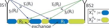
The insight underlying this lemma can be grasped by considering Fig. 2. It illustrates a policyπawhich satisfies
the lemma’s conditions if signal strength decays monotonically with distance from the serving base station – although part of our system model, this is not required to prove the lemma. Policyπbis constructed by merely
exchanging service regions
R
1,R
2between the two base stations. The constraints on the best and worst case signalstrengths ensure that this exchange is favorable for both base stations at all the associated user locations, which implies the following straightforward fact.
BS1 BS2
R2 R1
X :=π1a π 2
X :=a s (R )
_
1 1 s (R )
_ 2 2 s (R )
_1 2 s (R )_2 1
exchange
> >
Fig. 2.A sub-optimal load allocation policy.
Fact 1 Under the assumptions on
R
1andR
2 in Lemma 1, and the assumption that capacity is monotonicallyincreasing in SINR, the capacity from BS1 to any user in
R
2is greater than that to any user inR
1under thesameinterference regime, i.e., BS2 is transmitting or not. Similarly, the capacity from BS2 to any user in
R
1is greaterthan that to any user in
R
2, whether BS1 is transmitting or not.So, the exchange leaves the intensity of arrivals to BS1 and BS2 unchanged, and associates users to them which then can be served at higher capacity under the same interference regime. This allows us to construct a spatial coupling (i.e., by associating users in different regions) for networks under the two policies, showing that the average queue lengths are not increased. The details of this argument are in the appendix, and can be extended to other service disciplines, e.g., FCFS and LCFS.
Theorem 1. For the two base station model defined in Sec. 2, there exists a static load allocation policy minimizing
mean delay corresponding to a spatial threshold x∗∈[0,d]such that a user at location x is served by BS1 if x≤x∗
and by BS2 otherwise. This can also be expressed as a threshold on the ratio of received signal strengths from the two base stations.
Proof Sketch:Since traffic intensity measureλ(·)is non-atomic, if the service regions associated with the BS1
and BS2 are not contiguous, one can construct regions
R
1andR
2satisfying Lemma 1. Thus, a new policy canbe constructed by exchanging regions
R
1andR
2between the base stations’ service regions without increasingthe mean delay. This exchange operation can be repeated as long as the service areas are not contiguous. Thus an optimal policy must be defined by contiguous regions, i.e., specified by a spatial threshold. Since the ratio of the received signal strengths is strictly decreasing or increasing with the received signal strength (or distance) from a base station, the policy also be implemented as a threshold on this ratio.
Note that optimal static load allocation policies need not necessarily be unique. For example, consider the case when user requests are distributed homogeneously on the line segment joining the two base stations. If the optimal threshold does not correspond to the midpoint, then by symmetry, the policies that divide the service areas using thresholds at a distanced∗from BS1 andd∗from BS2 will result in identical mean user delays.
4
Optimal Threshold Trends
As a consequence of Theorem 1, we need only consider threshold-based static allocation policies. Fig. 1c exhibits the simulated mean user delay for varying thresholding policies as the (spatially homogeneous) arrival rate be-tween the base stations increases. The policies are characterized by the fraction of load served by BS1 with 0.5 corresponding to load balancing and 0.1 to only 10% of the load. As noted earlier, due to symmetry, the delay performance would be identical if the threshold were moved closer to BS2. For each arrival rate, the optimal load split, i.e., roughly achieving the minimum mean delay, is highlighted. We make the following observations:
1.The location of the optimal threshold is a function of the load on the system.
2.Except at very low loads, delay performance is improved by moving the threshold away from the mid-point, thus inducing asymmetrical loads on the two base stations.
interference is present, the capacity users see (particularly those far from either base station) can be substantially reduced by interference, and the fraction of time that base stations interfere with each other depends on the traffic and the load allocation policy. Thus, when arrival rate is low, the probability of the base stations being simulta-neously active is low; the base stations operate in an interference-free environment, and load balancing is roughly optimal. For higher arrival rates, performance is strongly impacted by interference, and skewing the load is bene-ficial. Intuitively, this skew reduces the utilization of one of the base stations, say BS1, and thus the interference it causes on BS2’s users, which reduces BS2’s utilization, in turn benefiting BS1. However, one cannot overdo this skew as serving users that are far away, and thus have poor received signal, is also detrimental. Finally, it is tempting to assume that as load increases, base stations are always busy and the role of dynamic coupling reduces. Yet, as can be seen, at high loads performance sensitivity is also high, and the gains of an optimal asymmetric split increase further. The optimal threshold reflects a complex tradeoff among dynamic interference, statistical multiplexing, and users’ signal strengths.
5
Optimizing the Threshold
In this section, we propose an approximation methodology for optimizing static load allocation policies for the wireless network model in Sec. 2, naturally extended toN base stations serving a possibly higher dimensional region. A policyπpartitions the service area such that base stationnhas service area
X
πn and overall arrival rate λn=λ(
X
nπ). Several technical challenges will be addressed. First, we approximate the Markovian model with uncountable state space by one with a countable state space, i.e., we will no longer keep track of the locations of users associated with each base station. This involves introducing an ‘effective’ rate forallusers associated with a base station which depends on the busy state of the remaining base stations. Thus, the model preserves the dynamic interference characteristics. Second, we propose an approach to upper/lower bound the performance for the approximated model. Finally, we propose optimizing performance over families of static policies that can be easily parametrized, e.g., for our one dimensional example, one need only determine the threshold. The subsequent section shows the accuracy of the proposed methodology is excellent. We also note that the approach is applicable to a broader set of problems with coupled queues or dynamic interference.5.1 Countable State-Space Approximation
We letQ~(t) = (Qn(t),n=1, . . . ,N)denote the number of active users at each base station at timet for our
ap-proximated process. For notational simplicity, we have suppressed its dependency onπ.As mentioned earlier, the capacity to a user depends onbothits current location and the interference profile it sees from neighboring base stations. We let~∆(t) = (∆n(t),n=1, . . . ,N)where∆n(t) =1(Qn(t)>0)denotes the status (idle or busy) or the
‘in-terference profile’ of the base stations. Note that~∆(t)can take 2Npossible values which we denote~δi,i=1, . . . ,2N.
Letcn(x,~δi)denote the actual capacity at which base stationncan serve a user at locationx∈
X
πn under interference
profile~δi.
The incremental time users spend in the system is inversely proportional to their service capacity. Thus, the mean rate at which users in a cell can be served depends on the steady state distribution of users that is induced in the cell (which differs from the distribution of arrivals). As shown in [24], the effective service capacity of a base station is given by the harmonic mean of the user capacities, when these are not time varying. In our approximate model, the effective capacity under interference profile~δidependsonlyon~δiand is given by
c~δi n =
Z
Xπ n
1
cn(x,~δi) λ(dx)
λn
!−1
,
theharmonic meanof the users service capacities under~δi weighted by the spatial distribution of arrivals to the
base station, i.e.,λ(dx)
λn .Since, in reality, each user does observe different rates over the course of time depending on
the activity level of the neighboring base station, these effective capacities are an approximation. However, users with low received signal strength tend to be located near the cell edge, and are also typically subject to high levels of inter-cell interference. Thus, in most cases, we expect this approximation to be reasonable. Since files have mean size of 1, the total service rateµ~δi
n at base stationnunder interference profile~δiis given byµ
~δi
n =c
~δi
n.We assume
the state for the uniformized discrete time Markov chain and~∆(k)the associated interference profile at discrete time stepk. The transition probabilities for the uniformized Markov chain are as follows. Suppose~Q(k) =~qhas associated interference profile~δi, i.e.,δin=1(qn>0)then
P(arrival to queuen|Q~(k) =~q) =λn η ,
P(departure from queuen|Q~(k) =~q) =µ
~δ i
n
η δ i n,
P(no change|Q~(k) =~q) =1−∑Nn=1λn+µ ~δ
i
nδin
η .
Note that, if it exists, the uniformized chain’s stationary distribution is identical to that of the original. Also, its evolution can be represented as a stochastic recursion
~
Q(k+1) =Q~(k) +~X(k), k=0,1, . . . ,
where~X(k) = (Xn(k),n=1,2, . . . ,N)denotes increments in the queues. An arrival into queuenat iterationkis
represented byXn(k) =1, a departure byXn(k) =−1 and if the transition corresponds to the self-loop,~X(k) =~0.
Note that~X(k)andQ~(k)are not independent, e.g., one can not have a departure from an empty queue. When the system is stable [25, 26], there is a stationary distribution for(Q~,~X)such that
~
Q=d g(~Q,~X):=Q~+~X (1)
where=d denotes equality in distribution.
5.2 Performance Bounds
Below, we describe our approach to bounding the system’s mean sum-queue length. The approach extends the work of [27] to coupled queuing systems and can also be used to bound other performance metrics, see [28] for more details. Bounds on the mean queue lengths in turn translate to bounds on the mean delay via Little’s Law.
Letψdenote a joint distribution for(Q~,~X)on
S
=S
~Q×S
~X⊆ZN+×ZN+satisfying (1) and with marginalsψQ~andψ~X. Eq. (1) can in this case be rewritten as
ψ~Q=ψg−1. (2)
We partition
S
~Qinto 2N regions where thesameset of queues are non-zero, i.e.,S
~δi :={~q:δin=1(qn>0),n=1, . . . ,N}fori=1, . . . ,2N.Letψ~δi andψ~δ~i Q,ψ
~δi ~
X be the conditional distributions for( ~
Q,~X)and its marginals given ~
Q∈
S
~δi. Note that for all states inS
~δi the queues share the same service rates, so follows Q~ is conditionallyindependent of~XgivenQ~ ∈
S
~δi, i.e.,ψ~δ
i
=ψ~δ
i ~
Qψ
~δi
~X, i=1, . . . ,2
N. (3)
We shall use multi-index notation in formulating our bounds. For~α∈ZN+and~Y ∈RN we let~Y~αdenote the
termYα1 1 . . .Y
αN
N , and let|~α|=∑nN=1αn. Forr∈Nwe define m~~β
δi=Eψ~~δi
X h
~X~βi,|~
β| ≤2randi=1, . . . ,2N. (4)
Given the transition probabilities on each region
S
~δi these can be easily computed. Bounds on mean sum-queue
length can be obtained by optimizing distributionsψsatisfying the following constraints:
Problem 1. Given
S
,S
Q~ andS
~Xsolve:sup/inf
ψ Eψ~Q "
N
∑
n=1
Qn
#
s.t. (2),(3),(4),
Eψ[1] =EψQ[1] =EψX[1] =1, (5)
Here,M(
S
),M(S
~Q), andM(S
~X)are sets of positive Borel measures supported onS
,S
Q, andS
X respectively, and(5) ensures they are probability measures. The parameterrcontrols the degree of accuracy of such bounds [29]. As
r→∞the distribution of~Xis specified exactly, in turn uniquely determining the distributions ofQ~ and and(~Q,~X). To allow numerical computation, we further relax Problem 1 based on joint moments of degree no higher than 2r. For all~α,~βsuch that|~α|+|~β| ≤2randk=1, . . . ,2Nwe define decision variables:
x~αk~β:=E[Q~~α~X~β|Q~ ∈
S
~δk]P(Q~ ∈
S
~δk).Note that the mean sum queue length can now be expressed as∑Nn=1∑2 N
k=1x ~en,0
k , where~enis the unit vector with a 1
for queuen.
Eq. (2), or equivalently (1), implies equality for all moments on the left and right hand sides. Note that
g(Q~,~X)~α= (~Q+~X)~α=
∑
|~γ1|+|γ~2|≤αg(~γ1,~γ2) ~α ~Q
~ γ1~X~γ2,
with Binomial coefficients{g(~γ1,~γ2)
~α }. So, we can relax the distributional constraint (2) to a constraint on moments
of order no higher than 2rgiving
2N
∑
k=1 x~kα,0=
2N
∑
k=1|~γ1|+
∑
|~γ2|≤αg(γ~1,~γ2)
~α x
~ γ1γ~1
k ,∀|~α| ≤2r. (7)
We also relax constraint (3) by equating the moments of the product distribution to the products of the moments
x~αk~β=m~β
δkx ~α,0
k ,∀|~α|+|~β| ≤2r,k=1, . . . ,2
N, (8)
which also subsumes (4). Constraint (5) can be directly expressed as:
2N
∑
k=1
x0k,0=1. (9)
Finally we need to ensure constraints (6) are satisfied by the moments/decision variables. Letxk={x
~α~β k ,|~α|+
|~β| ≤2r}, a moment sequence associated with the set
S
~δk for k=1, . . . ,2N. We denote the cone of momentssupported on
S
k=S
~δk×
S
XbyM
2r(S
k), and it’s closure byM
2r(S
k). So (6) translates to a moment constraintxk∈M
2r(S
k), ∀k=1, . . . ,2N.Such constraints can in turn be expressed as certain matrices being positive semidefinite.In general, a necessary condition for the sequencey={y~α~β,|~
α|+|~β| ≤2r}to be a valid truncated sequence of
moments is that the associated moment matrix, denotedMr(y), be positive semidefinite, i.e.,Mr(y)0 – see [27,
29] for details. Such constraints must be satisfied by the truncated moment sequences, i.e.,
Mr(xk)0, k=1, . . . ,2N. (10)
Additionally, note that
S
~δkcan be specified by an intersection of linear inequalities and so canS
k,i.e.,S
k=∩h∈Hk{h(~q,~x)≥0},whereHkdenotes a set linear functions defining
S
k.Clearly{xk}should also be a valid truncated moment sequencewhen restricted to each half plane{h(~q,~x)≥0}. Again it can be shown that a necessary condition for this to be the case is that an associated (localizing) moment matrix, denotedMr−1(h,xk), depending on the coefficients of the
hyperplanehandxkbe positive semidefinite, see [27, 29] for details. The corresponding set constraints is given by
Mr−1(h,xk)0,∀h∈Hk,k=1, . . . ,2N. (11)
Substituting our relaxed moment and semidefinite constraints into Problem 1 we obtain :
Problem 2. Givenm~~β
δi, |
~β| ≤2randi=1, . . . ,2N, the moments ofX, solve:
sup/ inf
{xk|k=1,...,2N}
2N
∑
k=1
N
∑
n=1 x~en,0
k
s.t. (7),(8),(9),(10),(11).
5.3 Determining Optimal Thresholds
As mentioned earlier, when policies can be easily parameterized, one can use these bounds to optimize perfor-mance. For our two base-station scenario, Theorem 1 shows the optimal static load allocation policy is a simple threshold. So for any threshold, Problem 2 can be solved to determine bounds on the mean delay, and a simple line search can be used to determine the threshold giving the smallest lower bound on the mean delay. In the case of the three base station network considered in the sequel, we parametrize policies based on weights associated with the base stations, as described in Sec. 6.3.
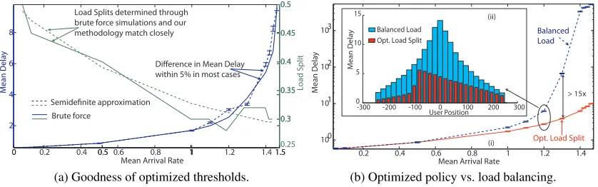
Fig. 3a exhibits the computed approximate optimal thresholds versus those obtained via brute force simulation for our two base station model. Semidefinite optimization problems associated with relaxations of order 2 were solved using [30] and [31] to determine the necessary bounds. As can be seen both load splits (thresholds) and resulting mean delay performance are very close, supporting the accuracy of our optimization methodology. The optimization approach however provides the flexibility to address complex traffic loads as well as systems with a larger number of base stations.
0.2 0.4 0.6 0.8 1 1.2 1.4
2 4 6 8
M
ean D
ela
y
Mean Arrival Rate
0 0.5 1 1.50.25
0.3 0.35 0.4 0.45 0.5
0 0.5 1 1.5
0.3 0.35 0.4 0.45 0.5
Load Split
Load Splits determined through brute force simulations and our methodology match closely
Difference in Mean Delay within 5% in most cases
Semidefinite approximation Brute force
(a) Goodness of optimized thresholds.
0.2 0.4 0.6 0.8 1 1.2 1.4
100 101 102 103
Mean Arrival Rate
M
ean D
ela
y
Opt. Load Split Balanced Load
-300 -200 -100 0 100 200 300
0 5 10 15
User Position
M
ean D
ela
y Balanced Load
Opt. Load Split
> 15x (ii)
(i)
(b) Optimized policy vs. load balancing.
Fig. 3.Performance of the optimized static user association policy.
6
Performance Comparison
6.1 Comparing Static Policies
Fig. 3b-i again illustrates the impact that the choice of threshold location has on delay performance. The user distribution is spatially homogeneous, so locating the threshold at the midpoint between the base stations corre-sponds to a static load balancing approach. As can be seen, the resultant mean user delays are greatly decreased by choosing an optimal threshold, particularly at moderate to high system loads. Fig. 3b-ii further exhibits the spatial distribution of user delays under the two schemes when the rate at which user requests arrive in the network is 1.2 per second. Surprisingly, skewing the load towards one base station does not result in a trade off where a subset of the users, e.g., at the heavily loaded base station, experience poor performance. Instead, under the optimal policy, the overall impact of inter-cell interference is reduced such that all users, irrespective of their spatial location or perceived signal strength, see improved performance on average.
6.2 Optimized Policy vs. Dynamic Strategies
Next we compare the performance of the optimal static policy versus the following three dynamic policies:
Greedy User:each new user joins the base station which offers the highest current service rate. This requires
knowledge of the new user’s capacity to each base station when the neighbor is active/idle and the number of users each is serving.
Greedy System:each new user is assigned to the base station so as to maximize the resulting current sum service
rate of the base stations. This policy is more complex than the Greedy User policy as in addition it requires knowledge of the capacity forallongoing users with and without interference.
Repacking:each time a user arrives or leaves, the assignments ofallusers are chosen so as to maximize sum
service rate of the base stations via a brute force search – the overheads and complexity of such a scheme would be unrealistically high, yet we hypothesize that it results in the best delay performance among non-anticipative dynamic schemes.
0.2 0.4 0.6 0.8 1 1.2 1.4 100
101 102 103
Mean Arrival Rate
M
ean D
ela
y
(a)
0 0.5 1 1.5
0 2 4 6 8 10 12
Mean Arrival Rate
M
ean D
ela
y
(b)
-3000 -200 -100 0 100 200 300
2 4 6 8 10 12 14 16 18
User Position
M
ean D
ela
y
(c)
> 6x
10% difference
Opt. Load Split
Greedy System Greedy User
Repacking Opt. Load Split
Opt. Load Split
Greedy System
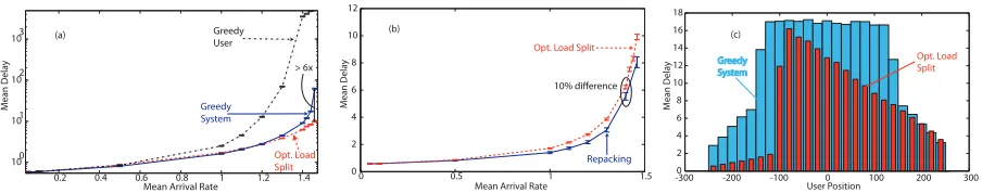
Fig. 4.Mean delay under optimized policy vs. (a) greedy schemes (log scale); (b) repacking scheme (linear scale);
(c) greedy system in terms of spatial distribution.
loads. Indeed, at high load, the mean delay of the static policy is 6 times lower than the greedy system policy which itself is orders of magnitude lower than the greedy user policy. As expected, the repacking policy shown in Fig. 4b (linear scale) is the best, but indeed very close to the optimal static policy.
Fig. 4c exhibits the spatial delay distribution under the system-level greedy scheme vs. the static policy. While the greedy policy exhibits perhaps desirable spatially symmetric performance, it is still the case that the optimal static policy gives better performance to all user locations.
6.3 Three Base Station Network
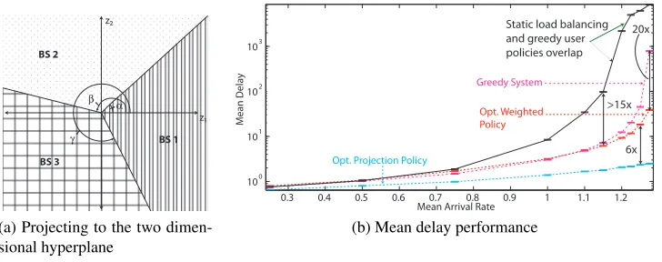
The three base station case can be used as a building block to develop a load allocation policy in a larger network. The number of base stations that can potentially serve a particular user request is unlikely to be very large. A load association policy that decides only between the three strongest base stations for each user request seems to be a reasonable tradeoff between complexity and performance. For the 2 dimensional three base station network described in Sec. 2.1, the form of the optimal static association policy is difficult to characterize. We compute the ‘optimal’ static association policy within a family of policies that can be easily parametrized.
Weighted signal strengths The first family of policies we consider is parametrized by base station weights. Each
base station is assigned a weight and a user is associated with the base station that offers the maximum weighted received signal strength. The weight associated with one of the base stations is set to 1, and a simple gradient descent is used to determine weights for the remaining base stations. The bounding methodology described in Sec. 5.2 is used to approximate the mean delay at each step of the gradient descent algorithm.
Pairwise optimization As an alternative to the methodology proposed above, we consider a family of policies
where modifying a single parameter while keeping the rest constant allows the load division between two base stations to be modified without affecting the set of users served by the other base station. Note that the policy presented in Sec. 6.3 does not possess this property as changing the weight associated with any base station po-tentially changes the load served by all three base stations. This property allows the sequential optimization of the policy parameters, and the optimal policy can be determined using a sequence of iterations where one parameter is adjusted in each iteration.
The vector of received signal strengths from the three base stations,~s(x) = (s1(x),s2(x),s3(x)), is projected
down on to the two dimensional hyperplane that passes through the origin and is orthogonal to the vector(1,1,1). The family of static policies that we consider divide this hyperplane into regions, and a base station serves all users whose projected signal strength vector falls in its region. The hyperplane is chosen such that users with identical relative received signal strengths from the base stations are mapped to the same point. The projected vector, after an orthogonal transformation is given by~z={z1,z2}, where
z1=
1
√
6(2s1(x)−s2(x)−s3(x))andz2= 1
√
2(s2(x)−s3(x)).
The hyperplane is divided into three regions by three rays extending from the origin, as shown in Fig. 5a. Each base station serves the region between two rays as illustrated in the figure. The rays are specified by the angles
α,β, andγthat they subtend with thez1axis, and these angles parametrize a policy within the family. Rotating one
z1 z2
α β
γ BS 1
BS 2
BS 3
(a) Projecting to the two dimen-sional hyperplane
0.3 0.4 0.5 0.6 0.7 0.8 0.9 1 1.1 1.2
100
101
102
103
Mean Arrival Rate
M
ean D
ela
y
Opt. Projection Policy
Greedy System
Opt. Weighted Policy
Static load balancing and greedy user policies overlap
>15x 20x
6x
(b) Mean delay performance
Fig. 5.Three base station network
chosen. Thus, each iteration lowers the overall mean delay experienced by users in the system, ensuring that the optimization procedure converges.
Fig. 5b exhibits the mean delay performance in a three base station network. The repacking policy for this case is a hard combinatorial problem to be solved upon each arrival/departure and so was infeasible. The static load balancing and the greedy user policies exhibit similar performance, i.e., overlap, while the optimized static (asymmetric) policy exhibits substantial performance gains. Even the greedy system policy (itself unrealistic in practice) achieves mean delays up to 20 times higher than the weighted signal strength based policy. The projection based policy performs significantly better than even the weighted signal strength policy, reducing the user perceived mean delay further by 6-10 times at high loads.
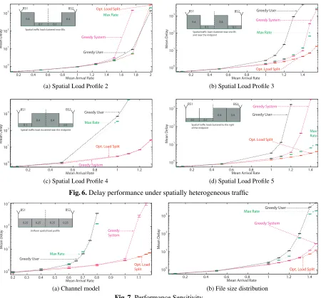
6.4 Heterogeneous Spatial Traffic Loads
Thus far, all the simulation results exhibited performance under spatially homogeneous user (load) distributions. In this section, we additionally consider various spatially non-homogeneous load profiles for the two base station scenario, as shown in Fig. 6a-6d. The line segment joining the two base stations is split into four quarters, and the load distribution is varied by varying the proportion of users in each quarter. Users in a particular quarter are uniformly distributed within that quarter. Load profiles 2 and 4 are symmetric with respect to the midpoint between the base stations. The users are concentrated near the base stations in profile 2, and the impact of inter-cell interference is diminished. The effective load on the network under this profile is lighter at a fixed user arrival rate compared to profile 4, where users are concentrated close to the midpoint and are strongly impacted by inter-cell interference. The load distribution under profiles 3 and 5 is asymmetric.
The optimized static policy performs consistently well under all spatial load profiles, and performs as well as or outperforms all the dynamic policies. This demonstrates its robustness to spatially heterogeneous traffic loads. Under load profile 3, for example, the optimized static policy outperforms all the other schemes by a wide margin. None of the other schemes perform well under all profiles, while our proposed scheme is able to infer the nature of the spatial load and adapt to it. The relative performance of the dynamic schemes can vary dramatically with the distribution of the spatial load. The greedy system scheme performs well under profiles 1 and 4. However, it is the worst among the schemes under load profile 2. Since the greedy system scheme tries to maximize the average throughput realized by all users in the system, it might deviate from a load balancing policy so as to ensure that a base station stays idle. However, since users cannot be reassigned, such decisions adversely affect long-term delay performance. The static max rate scheme performs well under load profile 2, where the effect of interference is minimal and under profile 4, where the spatial load is inherently asymmetric. It performs very poorly under the other spatial profiles.
6.5 Performance Sensitivity
Channel model: We use parameters that model cellular base stations in an urban environment. We simulate a
0.2 0.4 0.6 0.8 1 1.2 1.4 1.6 1.8 2
100
101
102
103
Mean Arrival Rate
M
ean
D
el
ay
Opt. Load Split
Greedy User Max Rate Greedy System BS1 BS2 0.4 0.1 0.1 0.4
Spatial traffic load clustered near BSs
(a) Spatial Load Profile 2
0.2 0.4 0.6 0.8 1 1.2 1.4
100
101
102
103
Mean Arrival Rate
M
ean D
ela
y
Opt. Load Split Greedy User Greedy System Max Rate BS1 BS2 0.4 0.1 0.4 0.1
Spatial traffic load clustered near one BS and near the midpoint
(b) Spatial Load Profile 3
0.2 0.4 0.6 0.8 1 1.2
100
101
102
103
Mean Arrival Rate
M
ean D
ela
y Max Rate
Greedy User
Greedy System Opt. Load Split
BS1 BS2
0.1
0.4 0.4 0.1
Spatial traffic load clustered near the midpoint
(c) Spatial Load Profile 4
0.2 0.4 0.6 0.8 1 1.2 1.4
100
101
102
103
Mean Arrival Rate
M ean D ela y Greedy User Greedy System Max Rate
Opt. Load Split
BS1 BS2
0.1 0.1
0.4 0.4
Spatial traffic load clustered to the right of the midpoint
(d) Spatial Load Profile 5
Fig. 6.Delay performance under spatially heterogeneous traffic
0.2 0.3 0.4 0.5 0.6 0.7 0.8 0.9 1 1.1
100
101
102
103
Mean Arrival Rate
M
ean D
ela
y
BS1 BS2
0.25 0.25 0.25 0.25
Uniform spatial load profile
Greedy User Max Rate Greedy System Opt. Load Split
(a) Channel model
0.2 0.4 0.6 0.8 1 1.2 1.4
100
101
102
103
Mean Arrival Rate
M ean D ela y Greedy User Max Rate Greedy System
Opt. Load Split
(b) File size distribution
Fig. 7.Performance Sensitivity
Long tailed file size distributions: In the process of determining the optimized static threshold, we still assume
that file sizes are exponentially distributed. We assume that the users’ file size requirements are log normally distributed with mean 5 MB, and variance 12.276×10⁶. The performance of the various schemes under a spatially homogeneous user distribution is shown in Fig. 7b. The relative performance of the different schemes is very similar to the case of exponential file sizes. The optimized static policy again results in the best performance, and appears to be robust to variations in the distribution of users’ file size requirements.
7
Conclusion
References
1. Borst, S., Hegde, N., Proutiere, A.: Capacity of wireless data networks with intra- and inter-cell mobility. In: INFOCOM. (2006)
2. Borst, S.: User-level performance of channel-aware scheduling in wireless data networks. In: INFOCOM. (2003) 3. Bonald, T., Borst, S., Proutiere, A.: Inter-cell coordination in wireless data networks. European Transactions on
Telecom-munications17(2006) 303–312
4. Das, S.K., et al.: A dynamic load balancing strategy for channel assignment using selective borrowing in cellular mobile environment. Wirel. Netw.3(5) (1997) 333–47
5. Bianchi, G., Tinnirello, I.: Improving load balancing mechanisms in wireless packet networks. In: IEEE ICC. Volume 2. (2002)
6. Yanmaz, E., et al.: Is there an optimum dynamic load balancing scheme? In: IEEE GTC. Volume 1. (2005)
7. Navaie, K., Yanikomeroglu, H.: Downlink joint base-station assignment and packet scheduling algorithm for cellular CDMA/TDMA networks. In: IEEE ICC. Volume 9. (2006) 4339–44
8. Das, S., et al.: Dynamic load balancing through coordinated scheduling in packet data systems. In: INFOCOM. (2003) 9. Sang, A., et al.: Coordinated load balancing, handoff/cell-site selection, and scheduling in multi-cell packet data systems.
In: ACM MobiCom. (2004) 302–14
10. Bonald, T., et al.: Inter-cell scheduling in wireless data networks. In: European Wireless Conference. (2005) 11. Borst, S., Saniee, I., Whiting, A.: Distributed dynamic load balancing in wireless networks. In: ITC. (2007) 1024–37 12. Zemlianov, A., et al.: Load balancing of best effort traffic in wirel. sys. supporting end nodes with dual mode capabilities.
In: CISS. (2005)
13. Bonald, T., et al.: Wireless data performance in multicell scenarios. In: SIGMETRICS. (2004)
14. Borst, S., Hegde, N., Proutiere, A.: Interacting queues with server selection and coordinated scheduling - application to cellular data networks. Annals of Operations Research170(1) (September 2009) 59–78
15. Jonckheere, M.: Stability of two interfering processors with load balancing. In: Third IInternational Conference on Performance Evaluation Methodologies and Tools. (2008)
16. Borst, S., et al.: Dynamic optimization in future cellular networks. Bell Labs Technical Journal10(2) (2005) 99–119 17. Borst, S.C.: Optimal probabilistic allocation of customer types to servers. In: ACM SIGMETRICS. (1995) 116–25 18. Fayolle, G., Lasnogorodski, R.: Two coupled processors: The reduction to a Riemann–Hilbert problem.
Wahrschein-lichkeitstheorie (3) (Jan. 1979) 1–27
19. Guillemin, F., Pinchon, D.: Analysis of generalized processor sharing systems with two classes of cus and exponential services. J. Appl. Prob.41(3) (2004) 832–858
20. Borst., S., et al.: Coupled processors with regularly varying service times. In: IEEE INFOCOM. Volume 1. (2000) 157–64 21. Borst, S., et al.: The asymptotic workload behavior of two coupled queues. Queueing Systems43(1-2) (January 2003)
81–102
22. Borst, S., Jonckheere, M., Leskel¨a, L.: Stability of parallel queueing systems with coupled service rates. Discrete Event Dynamic Systems18(4) (2008) 447–472
23. Rappaport, T.S.: Wireless Communications: Principles and Practice. Prentice Hall (2002)
24. Rengarajan, B., de Veciana, G.: Architecture and abstractions for environment and traffic aware system-level coordination of wireless networks: The downlink case. In: INFOCOM. (2008) 502–10
25. Borovkov, A., Foss, S.: Stochastically recursive sequences and their generalizations. Siberian Adv. in Math.2(1) (1992) 16–81
26. Loynes, R.: The stability of a queue with non-independent inter-arrival and service times. Proc. Cambr. Phil. Soc.58
(1962) 497–520
27. Bertsimas, D., Natarajan, K.: A semidefinite optimization approach to the steady-state analysis of queueing systems. Queueing Syst. Theory Appl.56(1) (2007) 27–39
28. Rengarajan, B., Caramanis, C., de Veciana, G.: Analyzing queueing systems with coupled processors through semidefinite programming.http://users.ece.utexas.edu/˜gustavo/papers/SdpCoupledQs.pdf(2008)
29. Lasserre, J.: Bounds on measures satisfying moment conditions. Annals of Applied Probability12(2002) 1114–1137 30. Henrion, D., Lasserre, J.: Gloptipoly: global optimization over polynomials with matlab and sedumi. ACM Transactions
on Mathematical Software29(2) (2003) 165–194
31. Sturm, J.F., the Advanced Optimization Laboratory at McMaster University: Sedumi version 1.1r3 (2006) See se-dumi.mcmaster.ca.
32. Marshall, A., Olkin, I.: Inequalities: Theory of Majorization and its Applications. New York: Academic Press (1979) 33. Stoyan, D.: Comparison Methods for Queues and Other Stochastic Models. New York: John Wiley (1983)
Appendix
Definition 1 ([32]).Letl,m∈Rn, and let l[1]≥ · · · ≥l[n]denote the components oflarranged in descending order.
l≺wmif
k
∑
i=1 l[i]≤
k
∑
i=1
m[i],k=1, . . . ,n
The vectorlis then said to beweakly majorizedbym.
Definition 2 ([33]).LetL,Mbe random vectors taking values inRn.Lisstochastically weak-majorizedbyM,
writtenL≺st
wM, if there exist random vectorsL˜ andM˜ taking values inRnwith the same probability laws asL
andMrespectively, withL˜ ≺wM˜ a.s.
Proof of Lemma 1:We will demonstrate that the policy πb, which is obtained fromπa by exchanging service
regions
R
1andR
2between the base stations, obtains a lower (or equal) mean delay, see Section 3. This is shownby constructing a pair of coupled processesU˜πa(t)andU˜πb(t), such that
˜
U
πb1 (t)⊆
U
˜πa
1 (t)and ˜
U
πb
2 (t)⊆
U
˜πa
2 (t), (12)
and such thatU˜πa(t)∼Uπa(t)andU˜πb(t)∼Uπb(t). It follows that associated queue length processesQ˜πa(t)and ˜
Qπb(t)satisfy similar properties with containment replaced with an inequality. By standard arguments, see [33],
this construction suffices to show thatQπb(t)isstochastically weak-majorizedbyQπa(t).Ast→∞this implies
πbachieves a lower (or equal) mean queue length, and thus, by Little’s Law, a lower (or equal) mean delay.
Note that the arrival rates associated with the exchanged service regions are equal so the arrival rate to each base station under the two policies are the same, i.e.,λ1=λ(
X
1πa) =λ(X
1πb)andλ2=λ(X
2πa) =λ(X
2πb). We couplearrivals of the two processesU˜πa(t)andU˜πb(t), as generated by a common Poisson process with intensityλ
1+λ2.
For convenience, we index user requests based on arrival times (including those in the system att=0), i.e., 1,2, . . . While arrival times for users to the two systems are identical, their locations may not be, whence we letxπa
i and
xπb
i denote the locations of theithrequest under policyπaandπbrespectively.
Supposex∈
U
˜πa1 (t)then letcπxa(t)be the capacity to the user under policyπa at timet taking into account
the state of the neighboring base station. Since users share capacity via processor sharing, effective service rate to users at locationsxandyunder the two policies is given byµπa(t,x) = cπxa(t)
Qπa
βπa(x)(t)
.andµπb(t,y) = c πb y (t)
Qπb βπb(y)(t)
. So the departure rate of users from BS1 under policyπais given by
µπa
1 (t) =
∑
x∈U˜πa 1 (t)
µπa(t,x).
We define the overall departure ratesµπa
2 (t),µ
πb
1 (t),andµ
πb
2 (t)analogously.
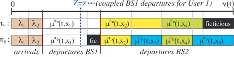
LetU˜πa(0) =U˜πb(0)so (12) holds at timet=0. Our construction will be such that if (12) holds at some time tthen it is satisfied after the next arrival/departure, while maintaining marginal dynamics that are consistent with systems associated with policiesπaandπb.Although the two systems see the same overall arrival rates they may
see different overall departure rates. In our construction we let
ν(t) =λ1+λ2+max(µπ1a(t),µ
πb
1 (t)) +max(µ
πa
2 (t),µ
πb
2 (t))
denote the current rate of events for thecoupled processesand allow fictitious events to ensure the marginal system processes have the correct dynamics. Let the time at which the next event occurs bet0andzbe a realization of a random variableZ, which is uniformly distributed on[0,ν(t)].The coupled process events are constructed as
follows:
μ (πat,x )
π :a
π :b μ (πbt,x ) λ1 λ2
λ2
μ (πat,x ) μ (πat,x )
πb
μ (t,x ) πb
μ (t,x ) μ (πbt,x )
πb
μ (t,x ) λ1
ν(t) 0
arrivals departures BS1 departures BS2
Z=z
1 1
2 2
3
3 4
4 ficticious
fic.
(coupled BS1 departures for User 1)
Fig. 8.Example coupling construction for arrivals/deparartures based on realization ofZ.
Arrivals:If 0≤z≤λ1, the next event is an arrival, say of usern , to BS1 under both policies. We let random
variablesXπa
n andX πb
is given byP(Xπa
n ∈A) = λ(A)
λ1 , for a measurable setA⊆
X
πa. The position of the user under policyπ
bis identical,
except ifXπa
n ∈
R
1. In this case, the user’s location falls withinR
2with a distributionP(Xnπb∈B|Xnπa∈R
1) =λλ((R2B)),whereB⊆
R
2.The states of the processes are updated accordingly. Ifλ1≤z≤λ1+λ2, the next event is an arrivalto BS2 under both policies, with the user’s location generated analogously to the above. In either case, arrivals to BS1 or BS2 occurs simultaneously for both policies, so (12) holds at timet0. Also under the above construction the spatial distribution of Poisson arrivals is maintained.
Departures:Ifλ1+λ2≤z≤λ1+λ2+max(µπ1a(t),µ
πb
1 (t)), the event is a potential departure from BS1. Consider
any userksuch thatxπb
k ∈
U
˜ πb1 (t). Since (12) holds, userkis also in the system under policyπa, i.e.,xπka∈
U
˜ πa1 (t).
Since (12) holds there are only three cases to consider:
1.
U
˜πb2 (t) =
U
˜πa
2 (t) =0/: BS2 is idle under both policies. Ifx
πa
k =x πb
k ,c πb
xπkb(t) =c πa
xπa k
(t). Otherwise,xπa
k ∈R1and
xπb
k ∈R2, so Fact 1 impliescπb
xπb k
(t)≥cπa
xπa k
(t).
2.
U
˜πb2 (t)6=0/,
U
˜πa
2 (t)6=0/: BS2 is transmitting under both policies, and, as in the previous case, we can argue that cπb
xπb k
(t)≥cπa
xπka(t). 3.
U
˜πb2 (t) =0/,
U
˜πa
2 (t)6=0/: In this case, users in BS1 see no interference under policyπbwhile they see interference
from BS2 under policyπa. Combining our conclusion in case 1 with the fact that the data rate at which users can be
served is an increasing function of the received signal to interference plus noise ratio, we see thatcπb
xπkb(t)≥c πa
xπa k
(t). Also, by assumption ˜Qπb
1 (t)≤Q˜
πa
1 (t), thusµπb(t,x
πb
k )≥µπa(t,x πa
k ).This permits us to couple Userk’s departure
such that if it leaves under policyπa, it also leaves under policyπb.To see this, consider Fig. 8 where[0,ν(t)]has
been subdivided based on the arrival rates and service rates of the users in the system under the two policies. If a user is present in both systems then a set of lengthµπa(t,xπa
k )for policyπais contained within one of length
µπb(t,xπb
k )for policyπb.If the user has already left the system under policyπa, the corresponding set for policy πbcan be arranged arbitrarily (need not be contiguous) within[0,ν(t)].Unused intervals correspond to dummy
events. Which departures (if any) occur for the two systems depend on which sets containz.However, clearly a departure of Userkfrom BS1 under policyπaresults in the same under policyπb unless it has already left the
system, and (12) still hold at timet0. If(λ1+λ2+max(µπ1a(t),µ
πb
1 (t)))≤z, the event is a potential departure from
BS2, and is treated analogously to departures from BS1.
Since relationship (12) holds after any future event, by induction the relationship holds for all times in the future. We show that the following relationship hold at any given time
1. ˜QP
1(t)≥Q˜
PE
1 (t)and ˜QP2(t)≥Q˜
PE
2 (t)
2. Corresponding to every user attached to BS1 under policyPE, there exists a user attached to BS1 under policy
P, that is served at lower rates both when BS2 is idle and active.
3. Corresponding to every user attached to BS2 under policyPE, there exists a user attached to BS2 under policy
P, that is served at lower rates both when BS1 is idle and active.
Now, consider a sequence of user arrivals and departures resulting from a static load allocation policy that associates users in regionr1 with base station 1, and users in region r2 with base station 2. We construct an
alternate sample path based on this sequence of user arrivals. User arrivals in regionr1are moved to instead arrive
in regionr2while still being served by base station 1, and user arrivals in regionr2are moved tor1and served by
base station 2. All other user arrivals are unchanged. Since the probability of user arrivals in regionr1is equal to
the probability of user arrivals inr2, and there are no correlations between user arrivals, the constructed sequence
of user arrivals is also representative of the arrival process.
The user queues associated with the two base stations evolve identically until a user arrives in either regionr1
orr2. As proved previously, this user is served at a higher rate in the alternate sample path. All other users currently
in the queues are served at exactly the same rates as in the original sample path as the queue lengths of the two queues are identical. As a result the user that arrived to one of the regionsr1orr2is served and leaves the system
earlier in the alternate sample path. This results in all the other remaining users in the system being served at the same or greater rate. Thus, all users in the alternate sample path perceive delays that are less than or equal to those in the original sample path.
Since both systems are ergodic, the sample mean of the user delays in both sample paths converge eventually to the expected values, and the expected user delay in the alternate sample path has to be lower or equal to that in the original. Note that this alternate sample path corresponds to a policy which associates users in regionr2with