IJSRSET1732192 | 15 April 2017 | Accepted : 22 April 2017 | March-April-2017 [(2)2: 685-698]
© 2017 IJSRSET | Volume 3 | Issue 2 | Print ISSN: 2395-1990 | Online ISSN : 2394-4099 Themed Section: Engineering and Technology
685
Image Enhancement using Morphological Operations
A. Sakila
1,
Dr. S. Vijayarani
2Research Scholar, Department of Computer Science, Bharathiar University, Coimbatore, Tamil Nadu, India
ABSTRACT
Today, Image Processing has become one of the popular and essential research domains in the field of computer science and information technology. Important tasks of image processing are image enhancement, image compression and information extraction. Image enhancement techniques are used to improve the quality of image where as information extraction techniques extract the statistical information about portion of an image or any particular image. Image compression is reducing the size of the digital image and allows more images to be stored in a computer disk. In this digital era, people can handle large amount of digital documents and with this documents we need to perform several tasks. Digital images may contain both machine printed documents and handwritten documents. Machine printed document images might have been produced using various technologies with good quality. A handwritten digital document has poor quality like blurred images, old handwritten manuscripts and handwritten variations, hence difficult to identify the texts. Hence the main objective of this paper is to enhance the handwritten image quality using various image enhancement techniques like Noise Removal, Contrast Stretching, Morphological Operations and Interpolations.
Keywords : Image Processing, Image Filters, Contrast Stretching, Morphological Operations, Interpolations.
I.
INTRODUCTION
Image Processing is process of digital images and perform some operations on it, in order to get an enhanced image or to extract some useful information from it [14], it involves the modification of digital data for improving the image qualities with the aid of computer. The processing helps in maximizing clarity, sharpness and details of features of interest towards information extraction and further analysis [13]. Digital images contain number of discrepancies like poor quality, and blurred images and old document images; hence image enhancement technique is used to improve the poor quality images into higher quality images. Image enhancement is the concept of improving the visual appearance of the image and provides the quality of images for other automated image processing techniques [5].The main objective of image enhancement is to modify one or more attributes of an image to make it more suitable for a given task [1]. The choice of attributes and modification depends on the specific task. Two extensive categories of image enhancement techniques are:
i. Spatial domain methods -It operates directly on pixels
ii. Frequency domain methods – It operates the Fourier transform of an image.
A. Applications of Image Enhancement
Some of the areas in which Image Enhancement has wide application are noted below [10] [11].
In atmospheric sciences, image enhancement is used to reduce the effects of haze, fog and turbulent weather for meteorological observations. Image enhancement helps in detecting shape and structure of remote objects in environment sensing. Satellite images undergo image restoration and enhancement to remove noise.
Astrophotography faces challenges due to light and noise pollution and this can be minimized by Image Enhancement. For real time sharpening and contrast enhancement several cameras have in-built Image Enhancement functions. However, numerous software, allow editing such images to provide better results.
In environmental sciences, picture improvement is utilized to decrease the impacts of murkiness, haze, and turbulent climate for meteorological perceptions. Picture improvement offers in distinguishing some assistance with shaping and structure of remote articles in environment detecting. Satellite pictures experience picture rebuilding and improvement to evacuate clamor.
In legal sciences, pictures got from unique mark location, security recordings examination and wrongdoing scene examinations are upgraded to use in distinguishing proof of guilty parties and insurance of casualties.
In oceanography the investigation of pictures uncovers intriguing elements of water stream, silt focus, geomorphology and bathymetric examples to give some examples. These elements are all the more plainly noticeable in pictures that are digitally upgraded to defeat the issue of moving targets [10, 11].
Supplementary fields including law enforcement, microbiology, biomedicine, bacteriology, etc., benefit from image enhancement techniques. The remaining portion of the paper is organized as follows. In Section 2 presents the review of literature and other approaches that have been employed to document image enhancement. Section 3 provides detailed description of the methodology. Image enhancement results are specified in Section 4. Section 5 gives the conclusion.
II.
METHODS AND MATERIAL
2. Related Works
Reza Farrahi, et.al [2] has combined the ICA method and the diffusion method. Double-sided degraded document images are based on the idea of general diffusion originating from several sources, a defect model for generating the physical defects in the documents is proposed. Subjective and objective evaluations are performed on both the degradation
model and the restoration method. Restoration model generates the document images and real documents. In addition to recovering the main text the restoration method can provide other useful information, such as simultaneous outputs.
G. Agam et.al [3] has proposed enhancement techniques on a subset of historical documents obtained from the Yad Vashem Holocaust museum. It is evaluated both qualitatively and quantitatively and compared to the commercial grade DjVu algorithm using various degradation models. The degradations are handled in a generic way by using either a min-max or probabilistic model (EM). They produced enhanced result which allows for a continuous set of views and that can be controlled by two interactive parameters. The first parameter controls the decision threshold of the foreground separation process and the second controls the blending factor of the display.
Zhengyou Zhanget.al [4] has developed a robust feature-based technique and this is used for automatic stitch multiple overlapping images. These images are taken from white board using digital cameras. The procedure consists of Edge detection, Hough transform, Quadrangle formation, Quadrangle verification, and Quadrangle refining. The physical aspect ratio of white board is determined by the Geometry of a Rectangle, images enhancing, Estimates the focal Length and Rectangle’s Aspect Ratio. Image enhancement is done by two steps whereas the first step makes the background white uniformly and in the second step it reduces the image noise and increases the color saturation of the pen strokes.
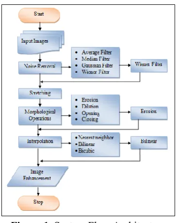
3. Image Enhancement
Figure 1. System Flow Architecture
3.1 Input Images
Different types of handwritten images are consider for this research work and it can be different image size and various image formats, i.e. JPG/JPEG, PNG, BMP, GIF and TIFF.
3.2 Grey Scale Conversions
Grey scale conversion is a pre-processing technique which converts the RGB image in to grayscale. The intensity of a pixel is expressed within a given range between a minimum and a maximum. Grayscale images have many shades of gray in between. The intensity of light at each pixel is measured in the
electromagnetic
spectrum
which produces the Grayscale images [7]. Figure 3.2 illustrates the grey scale conversion. The formula used to convert the color image into grayscale image is given below.Grayscale= (Red + Green + Blue) / 3
3.3 Noise removal
The acquired image is processed to remove any noise that may have incurred in the image during the time of acquisition or during the time of transmission. A color image will be converted to a gray image before proceeding with the noise removal procedure. The de-noised image is then converted to a binary image with suitable threshold. Noise removal is an important aspect of image quality and it is also called as image smoothing.
Filtering in image processing is a basis
function that is used for interpolation,
noise removal
and resembling [8]. Various filtering techniques are available for noise removal. Some of them are mean (linear), median (non-linear), average, Gaussian, wiener and adaptive. In this work, four filtering techniques namely Average, Median, Gaussian and Wiener filter are used and their performances are analyzed.3.3.1 Average Filtering
Average filters are commonly used in image processing to enhance image by removing noise without significantly blurring the structures in the image. It is more selective in preserving edges. The true color image is converted into grayscale. First noise is removed and then motion blurred images are converted with less blurring and finally blurred image is sharpened using linear function. This filter removes the noise in the images by using speech signal of interest (SOI) x (n) from the observation signal y (n) which is corrupted by the noise v (n),
y (n) = x(n) + v(n)
Where v (n) is the additive noise, which is a Gaussian random process. It is assumed that the noise v (n) is uncorrelated with the SOI signal x (n).
3.3.2 Median Filter
Noise removal from image using nonlinear filtering technique, non linear filter is a median filter. Noise reduction is a typical pre-processing step to improve the image results of later processing. An image containing different types of noise will have dark pixels in bright regions and bright pixels in dark regions. Median filter processes the corrupted images by detecting the impulse noise. Its mathematical analysis is relatively complex for the image with random noise.
Where is input noise power (the variance), n is the size of the median filtering mask, f (n) is the function of the noise density.
Gaussian filter removes noise from the images. It has the properties of step function in input, while minimizing the rise and fall time. This step is closely connected to the fact that the Gaussian filter has the minimum possible group delay. Gaussian filter as the sinc is also known as ideal frequency domain filter. It modifies the input image by convolution with a Gaussian function.
√
In two dimensions, it is the product of two such Gaussians, one in each dimension
√
Where and is the distance from source in the horizontal and vertical axis, is the standard deviation of the Gaussian distribution [7].
3.3.4 Wiener Filter
Wiener filter is used to removing noise and linear estimation of the original image; it removes the additive noise and inverts the blurring simultaneously [3] [9].
where are respectively power spectra of the original image and the additive noise, and is the blurring filter. These filters performance are analyzed and found that the wiener filter efficiency is better than other filters with its highest accuracy values by using PSNR (Peak Signal to Noise Ratio)[17].
3.4 Contrast Stretching
Contrast stretching is a simple image enhancement techniques, it is also called as image normalization. It used to improve the contrast of a low quality image by stretching the range of intensity values. This technique fairly effective if properly utilized and measures the difference in optic density, radiation transmission, pixel brightness or other parameters between two images.
3.5 Morphological Operation
Collection of non-linear operations is known as morphological operation, it related to the shape or morphology of features in an original image [15]. Dilation, erosion, opening and closing are basic morphological processing operators.
3.5.1 Erosion
Erosion “shrinks” or “removes” objects in a binary image. With A and B assets, the erosion of A by B is defined as
{ }
The erosion of A by B is the set of all points z such that B, translated by z, is contained in A, where set B is a structuring element. A 486x486 binary image of a wire-bond mask and images eroded using square structuring elements of sizes 11x11, 15x15and 45x45 pixels whose components were all ones.
3.5.2 Dilation
Dilation thickens or enlarges the objects in a binary image, which is based on set operations and therefore is a nonlinear operation. Dilation is defined as
{ ̂ }
This equation is based on reflecting B about its origin and shifting this reflection by z. The dilation of A by B then is the set of all displacements z, such that and an overlap by at least one element.
3.5.3 Opening
It generally smoothes the contour of an object and eliminate thin protrusions. The opening of a set A by structuring element B is defined as
Therefore, the opening A by B is the erosion of A by B, followed by a dilation of the result by B.
3.5.4 Closing
the contour. The closing of a set A by structuring element B is defined as
Therefore, the closing A by B is the dilation of A by B, followed by an erosion of the result by B.
3.6 Interpolation
Image interpolation is the process of enlarging an image which is more visible and clear, the size of the new or constructed image depends on the interpolation ratio of the image. This process has been using Document images, Satellite images, biomedical images, and agricultural images. Three different types of interpolation methods are used for enlarging digital images. They are nearest neighbor, bilinear and bicubic interpolation methods and these methods are using different image resolution. Most of the assumptions applied to reduce interpolated image resolution due to the low pass filtering process involved into their operations.
3.6.1 Nearest neighbour interpolation
Nearest neighbor is a simplest interpolation, which is interpolated output pixel is assigned the value of the nearest sample point in the input image. The interpolation kernel for the nearest neighbor is
{
The frequency response of the nearest neighbor kernel is H(ω) = sinc (ω/2). Although this method is very efficient, the quality of the image is very poor.
3.6.2 Bilinear interpolation
Bilinear interpolation is used to know values at random position from the weighted average of the four closest pixels to the specified input coordinates and assigns that value to the output coordinates. Two linear interpolations are performed in one direction and next linear interpolation is performed in the perpendicular direction. The interpolation kernel is given as
{
X is the distance between two points to be interpolated
3.6.3Bicubic interpolation
The bicubic interpolation is advancement over the cubic interpolation in two dimensional regular grids. The interpolated surface is smoother than bilinear interpolation and nearest-neighbor interpolation. It uses polynomials, cubic or cubic convolution algorithm. It determines the grey level value from the weighted average of the 16 closest pixels to the specified input coordinates, and assigns that value to the output coordinates, the first four, one-dimension. For bicubic Interpolation, number of grid points needed to evaluate the interpolation function is 16, two grid points on either side of the point under consideration for both horizontal and perpendicular direction. The bicubic convolution interpolation kernel is given as
{
Where a is generally taken as -0.5 to -0.75.
III.
RESULTS AND DISCUSSION
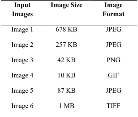
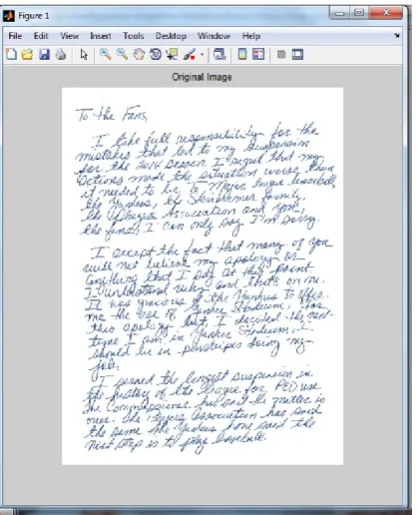
This work enhanced the document images using various morphological techniques. Different types of handwritten images taken for this analysis. Table 1 gives the Input image details. Figure 2 shows the original handwritten image.
TABLE I. Input Image Size and theirFormats
Input Images
Image Size Image Format
Image 1 678 KB JPEG
Image 2 257 KB JPEG
Image 3 42 KB PNG
Image 4 10 KB GIF
Image 5 87 KB JPEG
Figure 2. Input Image
4.1 Filtering Result
A. Performance Analysis of Filters
To analyze the performance of the filters, the PSNR and SSIM factors are used. Table 2 is presents, wiener filter performance is better than other filters based on its highest accuracy values i.e. PSNR (Peak Signal to Noise Ratio).
Table 2: Performance Analysis of Filters
Input images
Average Median Gaussian Wiener
PSNR SSIM PSNR SSIM PSNR SSIM PSNR SSIM
Image1 23.14 21.60 23.62 21.62 21.46 19.19 30.05 29.69
Image2 31.55 29.09 35.23 32.22 28.03 26.02 36.23 34.90
Image3 26.08 24.51 29.84 27.82 23.25 18.38 39.33 37.90
Image4 23.25 22.31 24.47 21.64 22.07 20.31 24.89 21.13
Image5 20.81 18.68 20.63 17.83 19.93 17.98 26.73 24.71
Image6 25.53 23.76 31.45 24.12 24.12 23.62 37.17 26.74
Figure 3: Performance Analysis of Filters 0
5 10 15 20 25 30 35 40 45
PSNR SSIM PSNR SSIM PSNR SSIM PSNR SSIM
Average Median Gaussian Wiener
Per
fo
rm
an
ce
m
ea
su
re
s
Filters
Performance Analysis for Filters
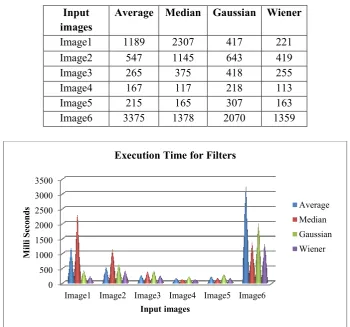
B. Execution time for filters
Table 3 gives the execution time required for the filters; wiener filter has required minimum execution time than other filters. Figure 4 shows the execution time for filters and Figure 5 displays the filtering results.
Table 3: Execution Time for Filters
Input images
Average Median Gaussian Wiener
Image1 1189 2307 417 221
Image2 547 1145 643 419
Image3 265 375 418 255
Image4 167 117 218 113
Image5 215 165 307 163
Image6 3375 1378 2070 1359
Figure 4: Execution Time for Filters 0
500 1000 1500 2000 2500 3000 3500
Image1 Image2 Image3 Image4 Image5 Image6
M
il
li
S
ec
on
ds
Input images
Execution Time for Filters
Figure 5: Filtering Results (1.Average, 2.Median, 3.Gaussian, 4.Wiener)
4.2 Contrast Stretching
Figure 6 represents the Contrast Stretching results.
Figure 7. Contrast Stretching results
4.3 Morphological Operation
C. Performance Analysis of Morphological Operation
than other morphological transformations. Figure 8 shows the Performance of Morphological Operations.
Table 4: Performance Analysis of Morphological Operations Input
images
Dilation Erosion Closing Opening PSNR SSIM PSNR SSIM PSNR SSIM PSNR SSIM
Image1 24.07 22.91 18.20 17.76 15.45 13.87 19.80 19.22
Image2 34.76 34.40 22.21 22.09 20.61 19.97 24.69 24.48 Image3 34.97 34.55 22.11 21.79 18.94 18.42 24.04 23.67
Image4 23.82 22.98 20.98 20.84 23.82 22.98 21.38 21.20
Image5 23.73 23.20 17.97 17.88 14.32 13.17 19.57 19.40 Image6 28.01 27.61 16.71 16.58 16.30 15.66 19.91 19.71
Figure 8: Performance Analysis of Morphological Operations
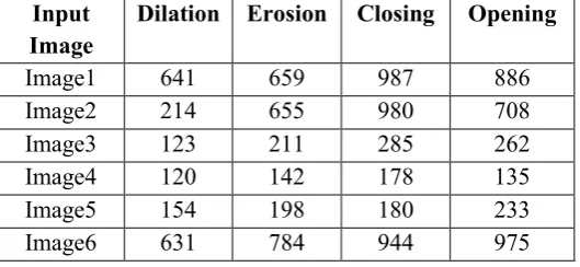
D. Execution Time for Morphological Operations
From Table 5, it is found that erosion has required minimum execution time than other morphological operations. Figure 9 represents the execution time required for morphological operations. Figure 10 displays the results for Morphological Operations.
Table 5: Execution Time for Morphological Operations
Input Image
Dilation Erosion Closing Opening
Image1 641 659 987 886
Image2 214 655 980 708
Image3 123 211 285 262
Image4 120 142 178 135
Image5 154 198 180 233
Image6 631 784 944 975
0 10 20 30 40
PSNR SSIM PSNR SSIM PSNR SSIM PSNR SSIM Dilation Erosion Closing Opening
Per
fo
rm
an
ce
M
ea
su
re
s
Morphological Operators
Performance analysis of Morphological Operators
Figure 9: Execution Time for Morphological Operations
Figure 10 : Result for Morphological Operations (A. Dilation, B. Erosion, C. Opening, D. Closing)
0 100 200 300 400 500 600 700 800 900 1000
Image1 Image2 Image3 Image4 Image5 Image6
Mi
ll
i Se
co
nds
Input Images
Execution Time for Morphological Operators
4.4 Interpolations
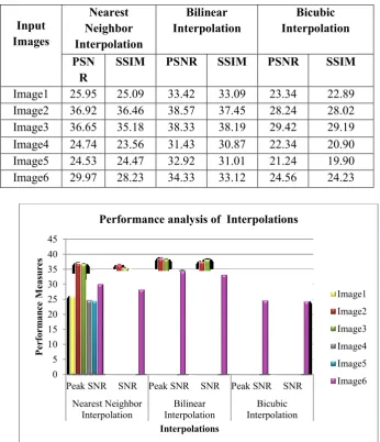
E. Performance analysis of Interpolations
Interpolation accuracy and execution time are considered as the performance measures of interpolations. PSNR and SSIM are used for measuring the interpolation accuracy. Table 6 represents that bilinear interpolation is better than other interpolations. This is given in Figure 11.
Table 6: Performance analysis of Interpolations
Input Images
Nearest Neighbor Interpolation
Bilinear Interpolation
Bicubic Interpolation
PSN R
SSIM PSNR SSIM PSNR SSIM
Image1 25.95 25.09 33.42 33.09 23.34 22.89 Image2 36.92 36.46 38.57 37.45 28.24 28.02 Image3 36.65 35.18 38.33 38.19 29.42 29.19 Image4 24.74 23.56 31.43 30.87 22.34 20.90 Image5 24.53 24.47 32.92 31.01 21.24 19.90 Image6 29.97 28.23 34.33 33.12 24.56 24.23
Figure 11: Performance analysis of Interpolations
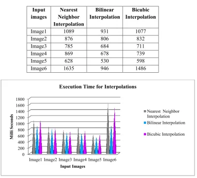
F: Execution Time for Interpolations
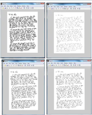
Bilinear Interpolation has required minimum execution time than other interpolations and this is given in table 6. Figure 12 represents the execution time for interpolations. Figure 13 displays the results for Nearest Neighbor Interpolation. Figure14 represents Bilinear Interpolation and Bicubic Interpolation result is given in Figure 14.
0 5 10 15 20 25 30 35 40 45
Peak SNR SNR Peak SNR SNR Peak SNR SNR Nearest Neighbor
Interpolation InterpolationBilinear InterpolationBicubic
Per
fo
rm
an
ce
M
ea
su
re
s
Interpolations
Performance analysis of Interpolations
Table 6: Execution Time for Interpolations
Input images
Nearest Neighbor Interpolation
Bilinear Interpolation
Bicubic Interpolation
Image1 1089 931 1077
Image2 876 806 832
Image3 785 684 711
Image4 869 678 739
Image5 628 530 598
Image6 1635 946 1486
Figure 12: Execution Time for Interpolations
Figure 13: Nearest Neighbor Interpolation 0
200 400 600 800 1000 1200 1400 1600 1800
Image1 Image2 Image3 Image4 Image5 Image6
M
il
li
S
ec
on
ds
Input Images
Execution Time for Interpolations
Figure 14: Bilinear Interpolation
Figure 15: Bicubic Interpolation
Figure16: Enhanced the particular portion of the original image
IV.
CONCLUSION
This work highlighted the various image
enhancement
techniques
which
are
used
particularly for improving the quality of an image.
Image enhancement plays a vital role for making
images better and interpretable. Usually images
contain low contrast and they are difficult to
understand and interpret. This article uses few
techniques that improve the quality of the image.
This paper discussed about the image enhancement
approaches and applications. This work was
analyzed on various historical printed document
images. Image enhancement techniques like
Filtering, contrast stretching, morphological
operations and interpolation are used and images
are enhanced for better visual quality. In future, old
manuscripts tear/ damage document images to be
will consider for image enhancement by using new
proposed algorithms and techniques.
V.
REFERENCES
[1]. Raman Maini, Himanshu Aggarwal “A
Comprehensive Review of Image Enhancement Techniques” Jounalof Computing, ISSN 2151-9617, VOLUME 2, ISSUE 3, MARCH 2010.
[2]. Reza Farrahi, Moghaddam and Mohamed Cheriet
“Low quality document image modeling and enhancement” IJDAR (2009) 11:183–201, DOI 10.1007/s10032-008-0076-2
[3]. G. Agam, G. Bal, G. Frieder and O. Frieder
“Degraded Document Image Enhancement”
[4]. Zhengyou Zhang and Li-wei He “Whiteboard
Scanning and Image Enhancement” IEEE
International Conference on Acoustics, Speech, and Signal Processing (ICASSP 2004), May 17-21, 2004
[5]. H. K. Sawant, Mahentra Deore “A Comprehensive
Review of Image Enhancement Techniques” International Journal of Computer Technology and Electronics Engineering (IJCTEE) Volume 1, Issue 2, ISSN 2249-6343.
[6]. S.Vijayarani, A.Sakila “Performance Comparison of
OCR Tools” International Journal of UbiComp (IJU), Vol.6, No.3, July 2015
[7]. https://en.wikipedia.org/wiki/Grayscale
[8].
http://embedded-computing.com/articles/comparing-nonlinear-filters-image-processing/
[9].
http://www.slideshare.net/sriAnkush/image-processing-saltpepper-noise
[10]. Zhengmao Ye, Habib Mohamadin, Su-Seng Pang,
Sitharama Iyengar “Contrast Enhancement and Clustering Segmentation of Gray Level Images with
Quantitative Information Evaluation” Weas
Transaction on Information Science & Application Vol. 5, pp.181, February 2008
[11]. Harmandeep Kaur Ranota and Prabhpreet Kaur
“Review and Analysis of Image Enhancement Techniques” International Journal of Information & Computation Technology, ISSN 0974-2239 Volume 4, Number 6 (2014), pp. 583-590, http://www. irphouse.com
[12]. Lawrence O’Gorman and Rangachar Kasturi
“Document Image Analysis” ISBN 0-8186-7802-X
[13]. Digital Image Processing for Image Enhancement
and Information Extraction
(http://civil.iisc.ernet.in/~nagesh/rs_docs/Imagef.pdf ).
[14].
http://math.ewha.ac.kr/~jylee/SciComp/dip-diml.yonsei/chap4-1.pdf
[15]. https://www.cs.auckland.ac.nz/courses/compsci773s