Volume 19 Number 4 pp. 359–366 C The Author(s) 2016. This is an Open Access article, distributed under the terms
of the Creative Commons Attribution licence (http://creativecommons.org/licenses/by/4.0/), which permits unrestricted re-use, distribution, and reproduction in any medium, provided the original work is properly cited. doi:10.1017/thg.2016.49
Temporal and Spatial Variations in the Twinning
Rate in Norway
Johan Fellman
Hanken School of Economics, Helsinki, Finland
Strong geographical variations have been noted in the twinning rate (TWR). In general, the rate is high among people of African origin, intermediate among Europeans, and low among most Asiatic populations. In Europe, there tends to be a south–north cline, with a progressive increase in the TWR from south to north and a minimum around the Basque provinces. The highest TWRs in Europe have been found among the Nordic populations. Furthermore, within larger populations, small isolated subpopulations have been identified to have extreme, mainly high, TWRs. In the study of the temporal variation of the TWR in Norway, we consider the period from 1900 to 2014. The regional variation of the TWR in Norway is analyzed for the different counties for two periods, 1916–1926 and 1960–1988. Heterogeneity between the regional TWRs in Norway during 1916–1926 was found, but the goodness of fit for the alternative spatial models was only slight. The optimal regression model for the TWR in Norway has the longitude and its square as regressors. According to this model, the spatial variation is distributed in a west–east direction. For 1960– 1988, no significant regional variation was observed. One may expect that the environmental and genetic differences between the counties in Norway have disappeared and that the regional TWRs have converged towards a common low level.
Keywords:assisted reproductive technology, geographical co-ordinates, multicollinearity, regression analysis, county
Strong geographical variations have been observed in the twinning rate (TWR). The TWR is high among people of African origin, intermediate among Europeans, and low among most Asiatic populations (Eriksson, 1973). In Eu-rope, there tends to be a progressive increase in the TWR from south to north, with a minimum around the Basque provinces on the border between Spain and France. The highest TWRs in Europe have been noted among the Nordic populations (Bulmer, 1970; Eriksson,1964, 1973; James1985). Furthermore, within larger populations some small isolated subpopulations have been identified to have extreme, mainly high, TWRs.
Fellman and Eriksson (1990) examined the regional vari-ation in the TWR in Finland for 1974–1983. Eriksson et al. (1993) presented a detailed study of the secular changes in the Nordic countries of Denmark, Finland, and Swe-den. In our studies of the regional variation of the TWR in Sweden, we have analyzed TWRs for the different counties (Eriksson & Fellman,2004; Fellman & Eriksson,2003,2004, 2005a,2009). In Fellman (2016), the temporal variation in the Norwegian TWR was compared with corresponding trends in the neighboring Nordic countries of Iceland and Denmark.
Material and Methods
Materials
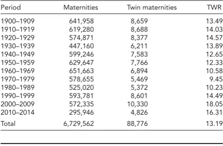
To evaluate the temporal variations in the TWR in Norway, we consider TWRs for 1900–2014 (Table 1). A deep trough can be found in 1960–1989. After 1990, a marked increase in the TWR is noted that cannot be explained by the slight increase in mean maternal age. The main cause of the re-covery of the TWR is noted to be the influence of assisted reproductive technologies (ART) and particularly the use of fertility-enhancing drugs on the commonly noted depen-dence between maternal age and TWR (Fellman & Eriks-son,2005a). Therefore, model building of normal TWRs should be based on data obtained before 1960.
The study of the spatial variation in the TWR is based on data grouped according to the Norwegian counties for 1916–1926. The available data are presented inTable 2. We
received 15 February 2016; accepted 31 March 2016. First published online 24 June 2016.
Address for correspondence: Professor Johan Fellman, Hanken School of Economics, Helsinki, Finland. E-mail:
TABLE 1
Temporal Variation in the Twinning Rate in Norway (1900–2014)
Period Maternities Twin maternities TWR
1900–1909 641,958 8,659 13.49
1910–1919 619,280 8,688 14.03
1920–1929 574,871 8,377 14.57
1930–1939 447,160 6,211 13.89
1940–1949 599,246 7,583 12.65
1950–1959 629,647 7,766 12.33
1960–1969 651,663 6,894 10.58
1970–1979 578,655 5,469 9.45
1980–1989 525,020 5,372 10.23
1990–1999 593,781 8,601 14.49
2000–2009 572,335 10,330 18.05
2010–2014 295,946 4,826 16.31
Total 6,729,562 88,776 13.19
TABLE 2
Regional Twinning Rates in Norway (1916–1926) Grouped According to the Norwegian Counties (or Fylkes)
Total Maternities TWR Latitude Longitude TW R
Östfold 40,599 14.1875 59.2833 11.2000 15.13 Akershus 92,584 14.0953 59.9333 10.7500 15.06 Hedmark 43,196 15.7304 60.7833 11.0500 15.11 Oppland 38,423 15.6937 61.1167 10.4167 15.00 Buskerud 31,625 14.5771 59.7333 10.1500 14.95 Vestfold 30,550 15.9411 59.2833 10.4167 15.00 Telemark 31,524 15.0044 59.2000 9.5500 14.84 Aust-Agder 17,058 14.7442 58.4667 8.7667 14.67 Vest-Agder 26,706 15.1092 58.1667 8.0000 14.49 Rogaland 38,287 12.3802 58.9500 5.7167 13.85 Hordaland 62,970 12.7125 60.3667 5.4000 13.75 Sogn og Fjordane 21,640 15.7344 61.2167 6.7833 14.19 Möre 41,548 15.7771 62.7500 7.2333 14.29 Sör-Tröndelag 43,436 14.1935 63.4167 10.3833 15.00 Nord-Tröndelag 23,075 15.0813 64.0500 11.7167 15.21 Nordland 49,318 14.3658 67.3000 14.5333 15.48 Troms 25,637 16.1487 69.6667 18.9333 15.44 Finnmark 15,091 12.9216 70.0667 29.7333 12.96 Total 673,266 14.544 61.8750 11.1519
Note: The latitudes and longitudes are the coordinates of the residences of the counties. TheTW Ris the observed TWR of the county, andTW Ris the estimated TWR of the county according to model (5). For details, see the text.
have considered a period for which the normal TWR rates are maximal. One may expect that the environmental and genetic differences have later disappeared and that the re-gional TWRs have converged towards a common low level. This may have influenced the TWR for 1960–1988.
Methods
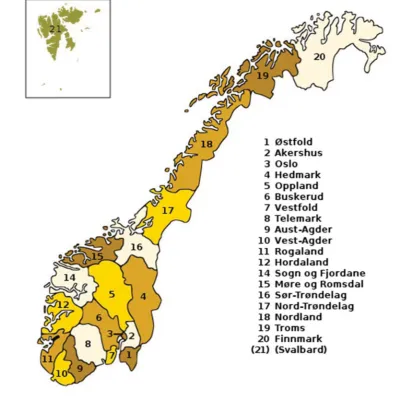
We applied different spatial regression models to the re-gional TWRs. The map of Norway and its counties is pre-sented inFigure 1. Following Fellman and Eriksson (2009), the location of the counties is defined as the geographic co-ordinates of the corresponding residences. The coco-ordinates for Norway are eastern longitude and northern latitude. The coordinates of the counties (residences) in Norway are also given inTable 2.
Multicollinearity
We analyzed the spatial variation in the TWR with alterna-tive regression models. The regressand is the TWR in the
different counties and the presumptive regressors are the longitude (meridian)M, and the latitudeL, and the regres-sors of second order, M2,L2, andLM. The regressorsM
andLare defined as deviations from their national cluster means, and consequently, the intercepts obtained are the es-timated TWRs in the center of the cluster.
The elongated or drawn-out format of Norway and the inclusion of the whole set of regressors, M, M2, L, L2, andLM, indicate that attention must be paid to the mul-ticollinearity between the regressors. Concerning regional studies of Swedish twins, this was also observed by Fell-man and Eriksson (2009). The multicollinearity pattern can show marked variations. Therefore, different measures based on the eigenvalues of the correlation matrix have been proposed in the literature. In the review of the litera-ture, Fellman (1981) and Fellman and Eriksson (2009) have given detailed presentations and analyses of different mea-sures of multicollinearity. In the following, a short presen-tation is given.
Consider a set of variables (regressors)u1,u2, ...,unand
their correlation matrix
C= ⎡ ⎢ ⎢ ⎢ ⎢ ⎢ ⎢ ⎣
1 c12 ... c1j ... c1n
c21 1 ... c2j ... c2n
. . . . . .
ci1 ci2 ... ci j ... cin
. . . . . .
cn1 cn2 ... cn j ... 1
⎤ ⎥ ⎥ ⎥ ⎥ ⎥ ⎥ ⎦ , (1)
whereci j=cor(ui,uj). If the variables are mutually
uncor-related the correlation matrix equals the identity matrix
I= ⎡ ⎢ ⎢ ⎢ ⎢ ⎢ ⎢ ⎣
1 0 ... 0 ... 0
0 1 ... 0 ... 0
. . . . . .
0 0 ... 1 ... 0
. . . . . .
0 0 ... 0 ... 1
⎤ ⎥ ⎥ ⎥ ⎥ ⎥ ⎥ ⎦ . (2)
The eigenvalues are obtained in the following way: Solve the equation
det(C−λI)=det ⎡ ⎢ ⎢ ⎢ ⎢ ⎢ ⎢ ⎣
1−λ c12 ... c1j ... c1n
c21 1−λ ... c2j ... c2n
. . . . . .
ci1 ci2 ... ci j ... cin
. . . . . .
cn1 cn2 ... cn j ... 1−λ
⎤ ⎥ ⎥ ⎥ ⎥ ⎥ ⎥ ⎦
=0. (3)
This equation is an algebraic equation of degreen. Con-sequently, it hasnrootsλ1, λ2, ...,λn, which are the
eigen-values of the matrix C. For every correlation matrix, the roots are real and non-negative andni=1λi=n. We
num-ber the roots such that 0≤λ1≤ λ2≤ ... ≤λn. If the
FIGURE 1
(Colour online) Map of Norway including the counties.
correlations between the variables, one speaks about mul-ticollinearity and there are small eigenvalues. The multi-collinearity causes reduced accuracy in the estimates. If λ1=0, then at least one exact linear relation between the regressors can be found and the correlation matrix is singu-lar and not all parameters are estimable.
Fellman (1981) discussed the pros and cons of the differ-ent multicollinearity measures. He stated that a good mea-sure should satisfy the following conditions: (a) the meamea-sure defines a critical level above (or below) which the corre-sponding correlation matrix should be considered strongly multicollinear; (b) the measure can be used for comparisons between different correlation matrices.
These properties imply that the measure must be (at least in a loose sense) ‘monotonic’ and the effect of the dimension of the matrix on the measure should not be too great. The measures of multicollinearity were also discussed in Fell-man and Eriksson (2009).
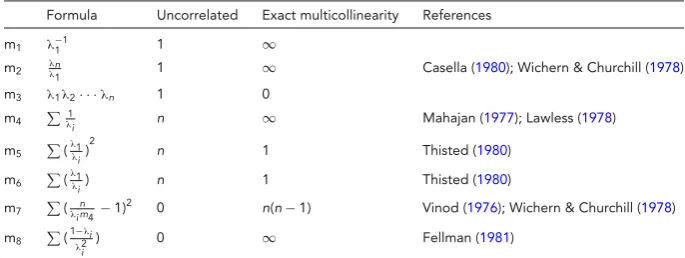
InTable 3, we present some commonly used measures of collinearity and their basic properties. The simplest mea-sure is the inverse of the minimum eigenvaluem1=λ−11. In the uncorrelated case,m1=1, but with increasing mul-ticollinearityλ1→0 andm1increases towards infinity.
The next measure, proposed by Wichern and Churchill (1978) and Casella (1980), ism2= λλn1. This is defined as the
condition numberof the matrix. In the uncorrelated case,
m2=1 and with increasing multicollinearitym2increases towards infinity.
The determinant of the correlation matrix, m3= det(C)=λ1λ2· · ·λn, has also been used as a measure of
multicollinearity. In the uncorrelated case,m3=1, but with increasing multicollinearitym3decreasestowards zero.
Mahajan et al. (1977) and Lawless (1978) considered the summ4=
1
λi. For uncorrelated variables, its value
TABLE 3
Definitions of Some Measures of Multicollinearity
Formula Uncorrelated Exact multicollinearity References
m1 λ−11 1 ∞
m2 λnλ1 1 ∞ Casella (1980); Wichern & Churchill (1978)
m3 λ1λ2· · ·λn 1 0
m4 λ1
i n ∞ Mahajan (1977); Lawless (1978)
m5 (λλ1i) 2
n 1 Thisted (1980)
m6 (λλ1i) n 1 Thisted (1980)
m7 (λi m4n −1)
2 0 n(n−1) Vinod (1976); Wichern & Churchill (1978)
m8 (1−λ2λi i
) 0 ∞ Fellman (1981)
Note: The measuresm3,m4andm8were chosen for this study. For details, see the text.
Thisted (1980) suggested two measures,m5=(λλ1i) 2
andm6=
(λ1
λi). These measures satisfy the inequalities
1<m5≤m6≤n. The equality signs hold only in the or-thogonal case. For uncorrelated variables, these measures obtain the valuen, and when the multicollinearity increases they converge towards one.
The measure m7=(λinm4 −1)2 was introduced by Vinod (1976). It is zero for complete orthogonal systems, but according to Vinod the components in the sum will be large for non-orthogonal data. However, the value ofm7 de-pends greatly on the relative proportions between the eigen-values and does not satisfy the assumption of a monotone function.
The measurem8=(1−λ2λi
i ) was introduced by Fellman
(1981), who presented arguments for its suitability as a mul-ticollinearity measure and proved thatm8≥0, with equal-ity in the orthogonal case, and thatlimλ1→0m8= ∞.
The measuresm1andm2are simple to handle, but their weakness is that they are mainly based on the smallest eigenvalue. Hence, any other small eigenvalues are almost ignored. The measurem3depends strongly on the dimen-sion of the matrix and is suitable only for matrices with low dimension. The advantage ofm4overm1andm2is that it takes into account the effect of several small eigenvalues. In addition, one can show that mathematically it has an evident connection with the estimation problem. Thisted (1980) recommendedm5in estimation andm6in predic-tion situapredic-tions. The main criticism against these measures is that they can be used if there is one extremely small eigen-value, but if there are several small eigenvalues the mea-sure is rather worthless. The meamea-surem7is useful only if we are dealing with a correlation matrix with only one small eigenvalue.
When we consider the variablesM,M2,L,L2, andLM, the dimension is low and several small eigenvalues may ex-ist. Consequently,m3,m4, andm8could be recommended and used in this study.
Results
Temporal Trends
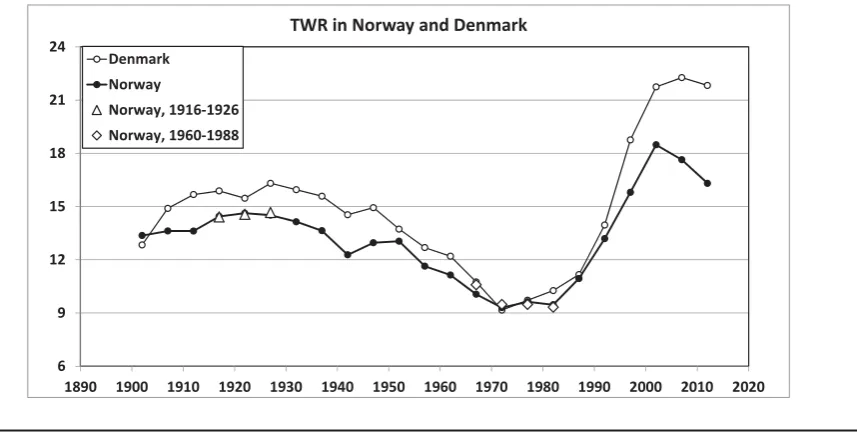
The temporal variation in the TWR in Norway (1900–2014) is presented inFigure 2. The TWR shows strong fluctua-tions. One observes that the TWR is rather constant until the 1950s, but there is a maximum in the 1910s and 1920s. There is a marked trough in the 1970s. After that, there is an increase up to the maximum 18.05 per 1,000 in 2000– 2009. The main cause of this recovery of the TWR seems to be the influence of ART (Fellman & Eriksson,2005a). A slight decrease in the TWR can be observed after 2009. Such recaptures can also be observed in other studies and are ex-plained by improved treatment techniques in order to avoid multiple maternities. For sake of comparison, the TWR for Denmark is included inFigure 2. The temporal trends for the TWRs in both countries are similar. The temporal trend of the seasonality in the TWR in Norway is discussed in Fellman and Eriksson (1999). More detailed studies of the TWR and general demographic studies of Denmark can be found in Eriksson and Fellman (1999); Fellman and Eriks-son (2005a); and Fellman (2015).
Regional Variation
The data during the periods 1916–1926 and 1960–1988 were used in the study of the regional heterogeneity, and these data are indicated inFigure 2. InTable 2, we have pre-sented the TWR distributed over the Norwegian counties for 1916–1926. When we applied aχ2test of the regional variation for the period 1916–1926, we obtainedχ2=56.8 with17degrees of freedom andp< .001, indicating statis-tically significant variations. Below, we follow Fellman and Eriksson (2009) and build spatial models of the regional variations.
We controlled as a check the regional TWRs for 1960– 1988 (Table 4) and for this period found no significant re-gional variations (χ2=21.59 with18degrees of freedom,
6 9 12 15 18 21 24
1890 1900 1910 1920 1930 1940 1950 1960 1970 1980 1990 2000 2010 2020
TWR in Norway and Denmark
Denmark
Norway
Norway, 1916-1926
Norway, 1960-1988
FIGURE 2
Temporal variation in the twinning rate in Norway (1900–2014). Note: The࢞symbol indicates data analyzed in the regional study. The
♦symbol indicates late regional data. For comparison sake, the TWR for Denmark is included in the figure. The temporal trends for the TWRs in both countries are similar.
TABLE 4
Regional Data in Norway for the Period 1960–1988.
County Maternities Latitude Longitude TWR
Östfold 85,929 59.2833 11.2000 9.356562 Akershus 80,239 59.9333 10.7500 9.745884 Oslo 212,837 59.9333 10.7500 10.20969 Hedmark 86,420 60.7833 11.0500 9.939829 Oppland 64,963 61.1167 10.4167 10.02109 Buskerud 75,724 59.7333 10.1500 9.996831 Vestfold 70,435 59.2833 10.4167 9.576205 Telemark 61,609 59.2000 9.5500 9.803762 Aust-Agder 36,920 58.4667 8.7667 9.507042 Vest-Agder 56,394 58.1667 8.0000 10.76356 Rogaland 135,336 58.9500 5.7167 9.871727 Hordaland 171,890 60.3667 5.4000 9.482809 Sogn og Fjordane 54,726 61.2167 6.7833 9.757702 Möre og Romsdal 97,585 62.7500 7.2333 9.90931 Sör-Tröndelag 102,912 63.4167 10.3833 9.4838 Nord-Tröndelag 56,646 64.0500 11.7167 9.515235 Nordland 104,007 67.3000 14.5333 10.15316 Troms 70,643 69.6667 18.9333 9.979757 Finnmark 41,273 70.0667 29.7333 8.795096 Total 1,666,488 61.7728 11.1307 9.822151
spatial models can only be applied in the data set for 1916– 1926. These findings can be compared with the results ob-tained by Fellman and Eriksson (2005b) that the regional TWRs for Sweden converged from 1750 to 1960 towards a common low level.
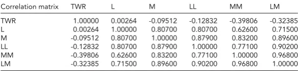
The elongated/drawn-out format of Norway suggests that we consider the multicollinearity in the regional mod-els for Norway. We calculated the correlation coefficients between the TWR and the regressorsM,M2,L,L2, andLM. The correlation matrix is given inTable 5. For the correla-tion matrix of the regressors, we obtainλ1=0.00175,λ2= 0.11089,λ3=0.15308,λ4=0.44883,andλ5=4.28945.
One eigenvalue is extremely small and at least two can be considered rather small.
The multicollinearity measures for our Norwegian data are presented in Table 6and a strong multicollinearity is obvious. Below, we define the optimal model consisted of the regressorsMandM2that we accept as optimal. For the
regressors in this model, the multicollinearity is markedly reduced. Now, the two eigenvalues areλ1=0.168015 and λ2=1.831985. The corresponding multicollinearity mea-sures for this reduced model are also included inTable 6. A comparison of the values ofm3,m4,andm8shows how much stronger the multicollinearity is for the larger model. Moving from the large model to the small,m3 increases from 0.0000566 to 0.307801, andm4andm8decrease from 590.4 to 6.50 and from 327166 to 29.2, respectively.Table 6 includes the Swedish data given by Fellman and Eriksson (2009). One observes that the multicollinearity in the Nor-wegian data is markedly stronger than in the Swedish data.
Regression Models
First we build the linear regression model for the total set of regressors. The obtained model is:
TWR=15.007+0.15197M+0.00975L+0.00090M2
+0.03401L2−0.04957LM. (4)
The goodness of fit of the model, measured with the ad-justed coefficient of determination, is ¯R2=0.080, indicat-ing a bad fit. This is supported by the low model test value
F=1.298. None of the parameter estimates is statistically
significant.
TABLE 5
Correlation Coefficients Between TWR and Regressors for the Norwegian Data
Correlation matrix TWR L M LL MM LM
TWR 1.00000 0.00264 -0.09512 -0.12832 -0.39806 -0.32385 L 0.00264 1.00000 0.80700 0.80700 0.62600 0.71500 M -0.09512 0.80700 1.00000 0.87900 0.83200 0.89600 LL -0.12832 0.80700 0.87900 1.00000 0.77100 0.90200 MM -0.39806 0.62600 0.83200 0.77100 1.00000 0.96800 LM -0.32385 0.71500 0.89600 0.90200 0.96800 1.00000
Note: A strong multicollinearity can be identified among the regressors.
TABLE 6
Multicollinearity Measuresm3,m4andm8for Our Norwegian Data
Norway Norway optimal Sweden Sweden, optimal
M,M2,L,L2,LM M,M2 M,M2,L,L2,LM M,M2,L,L2
m3 0.0000566 0.307801 0.015 0.159
m4 590.4 6.50 25.336 8.904
m8 327166.0 29.2 288.347 19.600
Note: One can observe that the multicollinearity for the optimal model is markedly re-duced and can be ignored. As a comparison, we include Swedish data presented in Fellman and Eriksson (2009). The Norwegian data show markedly stronger mul-ticollinearity.
gave a good fit, but all abridged models reduced the mul-ticollinearity. The best model obtained was a linear and a quadratic west-east model that contains the regressors
MandM2. The estimated model is:
TWR=15.12362+0.15482M−0.01461M2. (5)
The M2 parameter is significant and the M
parame-ter is almost significant. The standard errors are SEαˆ= 0.280353, SEβˆM =0.076354, and SEβˆM2 =0.005334. The adjusted coefficient of determination is ¯R2=0.251 and the
test statisticsF=3.855. Hence, the model is markedly bet-ter than Equation (4), but the goodness of fit for Equa-tion (5) is only slight.However, this model having a west-east trend has to be accepted as the optimal model. This model indicates the tendency of a central maximum for
M=5.298, and the value decreases in both western and eastern directions (cf.Figure 3). In fact, attempts to improve the model by includingM-terms of higher degree were quite fruitless.
We have explained the TWR with the geographical co-ordinates, and consequently, the pattern of the level curves is simple. If we assume that model (5) holds, we can then obtain parabolic level curves for the TWR. LetTW R0=R be a constant value, then the equation of the correspond-ing level curve isβMM+βM2M2+α−R=0, indicating a parabola with a vertical axis and the opening to the south. Furthermore, the axis obtained for the longitude is inde-pendent of the chosen TWR level. According to the pa-rameter estimates, the axis corresponds to thelongitude=
16.45◦E. Summing up, we consider Equation (5) as the best
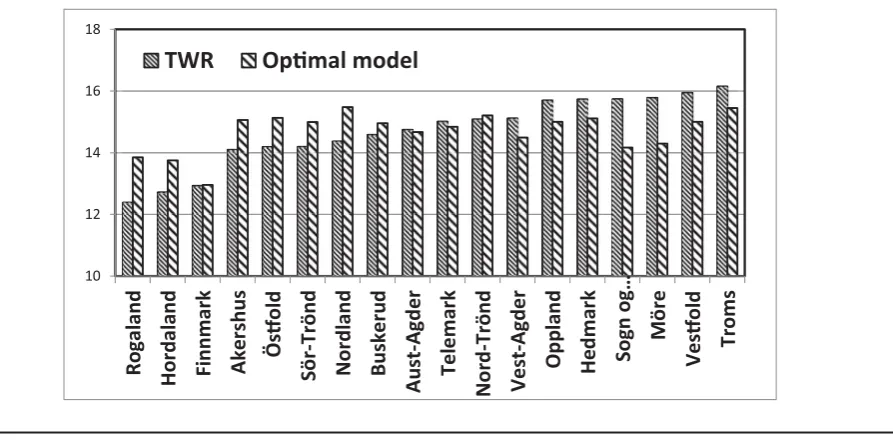
model, and the TWR estimates obtained are included in Table 2and presented inFigure 4. ForR=0 the level curve generates model (5).
11 12 13 14 15 16 17 18
0 5 10 15 20 25 30 35
Eastern longitude in degrees
Observed regional TWRs and opmal model
Opmal model Regional TWRs
FIGURE 3
Associations between regional TWRs (1916–1926) and the opti-mal model. Note: A slight east-western effect of second degree can be found. This model indicates the tendency of a central max-imum and decreases in both western and eastern directions. The TWRs for the central counties show values divergent from the model. This finding explains the slight goodness of fit. Attempts to improve the model by includingM-terms of higher degree were quite fruitless. Two level curves are included in the figure.
Discussion
10 12 14 16 18
Ro
galand
Ho
rd
ala
n
d
Fi
nnmark
Ake
rshus
Ös
old
Sör-Trönd
Nordland
Busker
u
d
Au
st
-Agde
r
Tel
e
ma
rk
Nor
d
-T
rö
nd
Vest-Agd
e
r
Op
p
la
n
d
He
dma
rk
Sogn og…
Mö
re
Ves
old
Tr
oms
TWR
Opmal model
FIGURE 4
Observed and estimated regional TWRs. Note: The counties are ordered according to increasing observed TWRs. The estimated TWRs are based on model (5). The low goodness of fit discussed in the text can be observed in this figure.
show higher TWR levels, but also strong discrepan-cies from the model (cf. Figure 3). Therefore, our find-ings corroborate the weak results observed in the spatial modeling.
The low regional variation of the TWRs for 1960– 1988 supports the finding that the regional TWRs for Sweden converged during the period from 1750 to 1960 towards a common low level (Fellman & Eriksson, 2005b).
Comparisons of the multicollinearity in this Norwegian study and in the study of Sweden presented in Fellman and Eriksson (2009) show that the multicollinearity is markedly stronger in Norway than in Sweden. This is obviously a re-sult of the fact that the two countries are almost of the same length, but Norway is much slimmer than Sweden. Further-more, the spatial study of the TWR in Sweden yielded more successful spatial models than this study of the regional TWRs in Norway.
James (1985) observed a positive correlation coefficient (Spearman’s) between the age-standardized TWR and lati-tude. He wondered whether this association of photoperi-odicity with latitude is relevant. As alternative factors, he suggested diet (milk consumption) and birth weight. Bul-mer (1970) has speculated that geographical variation in dizygotic TWRs in Europe may have some genetic basis. However, James (1985) stated that there is no reason to sup-pose that genetic clines in the Old World have been dupli-cated in the New World and the fact that the latitudinal vari-ation in DZ twinning and birth weight are similar in Europe and the United States suggests an environmental rather than a genetic cause.
Acknowledgments
This work was supported by grants from The Finnish So-ciety of Sciences and Letters and the Magnus Ehrnrooth Foundation.
References
Bulmer, M. G. (1970). The biology of the twinning in man. London: Oxford University Press.
Casella, G. (1980). Minimax ridge regression estimation. An-nals of Statistics, 8, 1036–1056.
Eriksson, A. W. (1964). Pituitary gonadotrophin and dizygotic twinning.Lancet, 2, 1298–1299.
Eriksson, A. W. (1973). Human twinning in and around the ˚
Aland Islands.Commentationes Biologicae,64, 1–159. Eriksson, A. W., Abbott, C., Kostense, P. J., & Fellman, J. O.
(1993). Secular changes of twinning rates in Nordic pop-ulations. In E. Iregren and R. Liljekvist (Eds.),Populations of the Nordic countries Human population biology from the present to the Mesolithic: Proceedings of the Second Seminar of Nordic Physical Anthropology Lund 1990(Report Series No. 46, pp. 113–135). Lund, Sweden: University of Lund, Institute of Archeology.
Eriksson, A. W., & Fellman, J. (1999). Seasonal variations of twin maternities in Denmark: Secular and regional differ-ences.Perspectives in Human Biology, 4, 213–221.
Eriksson, A. W., & Fellman, J. (2004). Demographic analysis of the variation in the rates of multiple maternities in Sweden since 1751.Human Biology, 76, 343–359.
Fellman, J. (1981).Leskinen’s preliminary orthogonalizing ridge estimator and a new measure of multicollinearity(Working Papers Swedish School of Economics and Business Admin-istration). Helsinki: Helsingfors.
Fellman, J. (2015). Temporal variation in rates of multiple ma-ternities in Denmark, 1850–2012.Twin Research and Hu-man Genetics, 18, 406–409.
Fellman, J. (2016). Historic demography of Iceland.British Journal of Medicine & Medical Research, 2, 1–13.
Fellman, J., & Eriksson, A. W. (1999). Secular changes in the seasonal patterns of births in Nordic countries.Perspectives in Human Biology,4, 203–212.
Fellman, J., & Eriksson, A. W. (2003). Temporal differences in the regional twinning rates in Sweden after 1750.Twin Re-search,6, 183–191.
Fellman, J., & Eriksson, A. W. (2004). Association between the rates of multiple maternities.Twin Research,7, 387–397. Fellman, J., & Eriksson, A. W. (2005a). Variations in the
maternal-age effect on twinning rates: The nordic experi-ence.Twin Research and Human Genetics, 8, 515–523. Fellman, J., & Eriksson, A. W. (2005b). The convergence of the
regional twinning rates in Sweden, 1751–1960.Twin Re-search and Human Genetics, 8, 163–172.
Fellman, J., & Eriksson, A. W. (2009). Spatial variation in the twinning rate in Sweden, 1751–1850.Twin Research and Human Genetics, 12, 583–590.
James, W. H. (1985). Dizygotic twinning, birth weight and latitude. Annals of Human Biology, 12, 441–447.
Lawless, J. F. (1978). Ridge and related estimation procedures: Theory and practice.Communications in Statistics — The-ory and Methods,A7, 139–164.
Mahajan, V., Jain, A. K., & Bergier, M. (1977). Parameter esti-mation in marketing models in presence of multicollinear-ity: An application of ridge regression.Journal of Marketing Research, 14, 586–591.
Thisted, R. A. (1980). Comment on Smith and Campbell (1980).Journal of American Statistical Association, 75, 81– 86.
Vinod, H. D. (1976). Application of new ridge regres-sion methods to a study of Bell system scale eco-nomics. Journal of American Statistical Association, 71, 835–841.