University of Pennsylvania
ScholarlyCommons
Publicly Accessible Penn Dissertations
1-1-2012
Statistical Methods for Human Microbiome Data
Analysis
Jun Chen
University of Pennsylvania, [email protected]
Follow this and additional works at:
http://repository.upenn.edu/edissertations
Part of the
Bioinformatics Commons,
Biostatistics Commons, and the
Microbiology Commons
This paper is posted at ScholarlyCommons.http://repository.upenn.edu/edissertations/497
For more information, please [email protected].
Recommended Citation
Chen, Jun, "Statistical Methods for Human Microbiome Data Analysis" (2012).Publicly Accessible Penn Dissertations. 497.
Statistical Methods for Human Microbiome Data Analysis
Abstract
The human microbiome is the totality of the microbes, their genetic elements and the interactions they have with surrounding environments throughout the human body. Studies have implicated the human microbiome in health and disease. Two central themes of human microbiome studies are to identify potential factors influencing the microbiome composition, and to define the relationship between microbiome features and biological or clinical outcomes. With the development of next generation sequencing technologies, the human microbiome composition can be interrogated using high-throughput DNA sequencing. One strategy
sequences the bacterial 16S ribosomal RNA gene for species identification. These 16S sequences are usually clustered into Operational Taxonomic Units (OTUs). Analysis of such OTU data raises several important statistical challenges, including taking into account the phylogenetic relationship among OTUs and modeling high-dimensional overdispersed count data. This dissertation presents three statistical methods developed specifically for 16S data analysis centering around the two themes. To test the association between overall microbiome composition and a covariate/an outcome, a testing procedure based on a generalized UniFrac distance was developed. The generalized UniFrac distance corrects the unduly weighting of classic UniFrac distances on either highly abundant or rare lineages, and was shown to be more powerful than the classic UniFracs. Under the framework of canonical correlation analysis (CCA), a structure-constrained sparse CCA was proposed to select the OTUs and their correlated covariates. A phylogenetic structure-constrained penalty function was imposed to induce certain smoothness on the linear coefficients according to the OTU phylogenetic relationship. Structure-constrained sparse CCA performed much better than sparse CCA in selecting relevant OTUs. Finally, a sparse Dirichlet-multinomial regression (SDMR) model was developed to link the microbiome composition to environmental covariates and to select the most important covariates and their affected OTUs. SDMR accounts for the overdispersion of OTU counts and uses a sparse group L1 penalty function to facilitate selection of covariates and OTUs simultaneously. These methods were illustrated using simulations as well as a real human gut microbiome data set from a study of dietary effects on gut microbiome composition.
Degree Type
Dissertation
Degree Name
Doctor of Philosophy (PhD)
Graduate Group
Genomics & Computational Biology
First Advisor
Hongzhe Li
Keywords
Subject Categories
STATISTICAL METHODS FOR HUMAN MICROBIOME DATA ANALYSIS
Jun Chen
A DISSERTATION
in
Genomics and Computational Biology
Presented to the Faculties of the University of Pennsylvania
in
Partial Fulfillment of the Requirements for the
Degree of Doctor of Philosophy
2012
Supervisor of Dissertation
Hongzhe Li, PhD, Professor of Biostatistics and Statistics
Graduate Group Chairperson
Maja Bucan, PhD, Professor of Genetics
Dissertation Committee
Mingyao Li, Assistant Professor of Biostatistics
Frederic Bushman, Professor of Microbiology
Nancy Zhang, Associate Professor of Statistics
STATISTICAL METHODS FOR HUMAN MICROBIOME DATA ANALYSIS
c
COPYRIGHT
2012
Jun Chen
This work is licensed under the
Creative Commons Attribution
NonCommercial-ShareAlike 3.0
License
To view a copy of this license, visit
ACKNOWLEDGEMENT
I would like to thank my advisor Hongzhe Li for his meticulous supervision of my research
during the last five years. I would have never been able to finish my dissertation without
his guidance. It is him who cultivates my deep interest in statistics and brings me to the
forefront of statistical methodological research. I have learned from him the essential skills
to be a good statistician, from writing a statistics paper to giving a clear presentation. Most
importantly, I have learned how to think statistically, which will prepare me well for future
independent research. I am very certain that his influence will carry over into my future
career. I would like to thank my collaborators Rick Bushman, Gary Wu and Jim Lewis for
providing me the microbiome data. I really enjoyed the collaborative experiences, which
not only helped me master existing statistical tools but also motivated me to develop new
statistical methods. These methods comprise the main part of this dissertation. My
heart-felt thanks also go to my committee members Mingyao Li, Rick Bushman, Nancy Zhang,
Li-san Wang and Carlo Maley for their time and efforts to serve on my committee. Their
valuable advices during committee meetings have helped me to improve my dissertation.
ABSTRACT
STATISTICAL METHODS FOR HUMAN MICROBIOME DATA ANALYSIS
Jun Chen
Hongzhe Li, PhD
The human microbiome is the totality of the microbes, their genetic elements and the
in-teractions they have with surrounding environments throughout the human body. Studies
have implicated the human microbiome in health and disease. Two central themes of human
microbiome studies are to identify potential factors influencing the microbiome
composi-tion, and to define the relationship between microbiome features and biological or clinical
outcomes. With the development of next generation sequencing technologies, the human
microbiome composition can be interrogated using high-throughput DNA sequencing. One
strategy sequences the bacterial 16S ribosomal RNA gene for species identification. These
16S sequences are usually clustered into Operational Taxonomic Units (OTUs). Analysis of
such OTU data raises several important statistical challenges, including taking into account
the phylogenetic relationship among OTUs and modeling high-dimensional overdispersed
count data. This dissertation presents three statistical methods developed specifically for
16S data analysis centering around the two themes. To test the association between
over-all microbiome composition and a covariate/an outcome, a testing procedure based on a
generalized UniFrac distance was developed. The generalized UniFrac distance corrects the
unduly weighting of classic UniFrac distances on either highly abundant or rare lineages, and
was shown to be more powerful than the classic UniFracs. Under the framework of
canon-ical correlation analysis (CCA), a structure-constrained sparse CCA was proposed to select
the OTUs and their correlated covariates. A phylogenetic structure-constrained penalty
function was imposed to induce certain smoothness on the linear coefficients according to
the OTU phylogenetic relationship. Structure-constrained sparse CCA performed much
regression (SDMR) model was developed to link the microbiome composition to
environ-mental covariates and to select the most important covariates and their affected OTUs.
SDMR accounts for the overdispersion of OTU counts and uses a sparse group l1 penalty
function to facilitate selection of covariates and OTUs simultaneously. These methods were
illustrated using simulations as well as a real human gut microbiome data set from a study
TABLE OF CONTENTS
ACKNOWLEDGEMENT . . . iv
ABSTRACT . . . v
LIST OF TABLES . . . ix
LIST OF ILLUSTRATIONS . . . xi
CHAPTER 1 : Introduction . . . 1
1.1 Human microbiome in health and disease . . . 1
1.2 Metagenomic approaches for human microbiome studies . . . 3
1.3 Motivation: The Penn gut microbiome project . . . 6
1.4 Characteristics of OTU/taxa data and statistical challenges . . . 7
1.5 Organization of the dissertation . . . 9
CHAPTER 2 : Associating Microbiome Composition with Environmental Covari-ates using Generalized UniFrac Distance . . . 13
2.1 Introduction . . . 13
2.2 Generalized UniFrac distance between two microbial communities . . . 16
2.3 Statistical test based on UniFrac distances . . . 18
2.4 Simulation studies . . . 19
2.5 Application to real data analysis . . . 24
2.6 Discussion . . . 27
CHAPTER 3 : Structure-Constrained Sparse Canonical Correlation Analysis for Mi-crobiome Data . . . 39
3.1 Introduction . . . 39
3.3 Structure-constrained sparse canonical correlation analysis . . . 43
3.4 Coordinate descent algorithm for ssCCA . . . 46
3.5 Simulation studies . . . 49
3.6 Application to real data analysis . . . 53
3.7 Discussion . . . 56
CHAPTER 4 : Variable Selection for Sparse Dirichlet-Multinomial Regression with Applications to Microbiome Data Analysis . . . 62
4.1 Introduction . . . 62
4.2 Dirichlet-multinomial model for microbiome composition data . . . 65
4.3 Dirichlet-multinomial regression for incorporating the covariate effects . . . 67
4.4 Variable selection for sparse Dirichlet-multinomial regression . . . 69
4.5 Simulation studies . . . 74
4.6 Application to real data analysis . . . 78
4.7 Discussion . . . 81
CHAPTER 5 : Future work . . . 92
APPENDIX . . . 95
LIST OF TABLES
TABLE 1 : Parameter values used in power study for 2D circle-based simulation. 30
TABLE 2 : Parameters used in ssCCA simulation studies. . . 58
TABLE 3 : Simulation results to evaluate ssCCA under models of different
asso-ciation signals, dimension sizes, cluster sizes, model misspecification
and complexity. . . 59
TABLE 4 : Comparison of the power of pseudo-F statistic based permutation
test and the DM model based likelihood ratio test in detecting the
covariate effect. . . 84
TABLE 5 : Comparison of sparse group `1 and`1 penalized procedures for
vari-able selection under Dirichlet-multinomial (DM), Dirichlet (D) and
multinomial (M) regression models. . . 85
TABLE 6 : Estimated regression coefficients from the sparse group`1 penalized
DM regression for the diet-gut microbiome data. . . 86
TABLE A1 : Differential OTUs between smokers and nonsmokers in the
LIST OF ILLUSTRATIONS
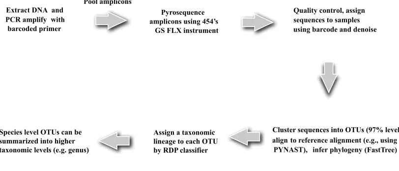
FIGURE 1 : Pipeline for 16S sequence data generation and processing. . . 11
FIGURE 2 : Characteristics of OTU data illustrated using the COMBO data. 12
FIGURE 3 : Two simulation strategies to evaluate the generalized UniFrac
dis-tance. . . 31
FIGURE 4 : Comparison of multinomial model and Dirichlet-multinomial model
for simulating OTU counts for an oropharyngeal microbial
commu-nity. . . 32
FIGURE 5 : Power comparison of different UniFrac variants for detecting
envi-ronmental effects using 2D circle based simulation. . . 33
FIGURE 6 : Power comparison of different UniFrac variants for detecting
envi-ronmental effects using tree based simulation. . . 34
FIGURE 7 : Power comparison of different UniFrac variants for detecting
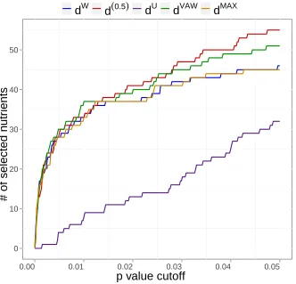
nutri-ent effects on gut microbiome composition. . . 35
FIGURE 8 : Comparison of different UniFrac variants for clustering samples
from smokers and nonsmokers. . . 36
FIGURE 9 : Sensitivity of generalized UniFrac distance to sampling depth. . . 37
FIGURE 10 : Effects of rarefaction on the power of association test. . . 38
FIGURE 11 : ROC curves for OTU selection using ssCCA and sCCA for Models
A1- H . . . 60
FIGURE 12 : Associating gut microbiome composition with dietary nutrient
in-takes using ssCCA. . . 61
FIGURE 13 : Effect of the tuning parameterc on variable selection. . . 87
FIGURE 14 : Effects of overdispersion and model-misspecification on the
FIGURE 15 : Effects of the number of relevant OTUs and the number of
covari-ates on the performance of sparse group`1 penalized DM regression
model. . . 89
FIGURE 16 : Model fit using the variables selected by the sparse groupl1
penal-ized DM regression model. . . 90
FIGURE 17 : Nutrient-genus association in the human gut identified by the sparse
group`1 penalized DM regression model. . . 91
FIGURE A1 : Power comparison of different UniFrac variants for detecting
en-vironmental effects using 2D circle based simulation and different
bin sizes for OTU formation. . . 98
FIGURE A2 : Power comparison of different UniFrac variants for detecting
en-vironmental effects using 2D circle based simulation and UPGMA
tree. . . 99
FIGURE A3 : Power comparison of different UniFrac variants for detecting
envi-ronmental effect using tree based simulation (all lineages). . . 100
FIGURE A4 : Effects of tree construction methods on generalized UniFrac
CHAPTER 1 : Introduction
1.1. Human microbiome in health and disease
We are not living alone. The human body is home to 10 trillion (1014) microbial cells,
exceeding at least 10-fold the number of human cells (Whitmanet al., 1998). The totality of
the microbes (microbiota), their genomes (metagenome) and the environment in which they
interact constitutes the humanmicrobiome(Cho and Blaser, 2012). The human microbiome
contains taxa from across the tree of life including bacteria, viruses, micro-eukaryotes, and
archaea, that interact with one another and with the host, greatly impacting the human
health and physiology (Clementeet al., 2012). The human microbiome encodes 100 times
more genes than the human genome, providing traits that humans did not need to evolve
on their own (Qin et al., 2010). The emerging concept of human “supra-organism” views
humans as a composite of microbial and human cells with human genetic landscape as an
aggregate of the genes in the human genome and the microbiome, and the human metabolic
features as a blend of human and microbial traits (Turnbaugh et al., 2007). In contrast
to the human genome, the human microbiome is highly variable. It displays substantial
intra-individual variation at different body sites (gut, skin, lung, vagina, oral cavity etc.),
inter-individual variation at the same body sites and intra-individual variation at different
times (Costello et al., 2009).
The human microbiome plays an important role in promoting human health. For
exam-ple, the human gut microbiome can harvest otherwise inaccessible nutrients, synthesize
certain vitamins, promote the proper development of the immune system and protect us
from pathogens (Turnbaugh et al., 2007). Increasingly more human microbiome studies
have implicated the human microbiome in the pathogenesis of many human diseases such
as obesity, diabetes, inflammatory bowel disease (IBD), irritable bowel syndrome (IBS),
vaginosis and even cancers (Cho and Blaser, 2012; Plottel and Blaser, 2011; Pflughoeft
Higher Firmicutes to Bacteroidetes ratios and reduced species diversity have been observed
in obese humans (Ley et al., 2005, 2006). Two recent studies found that the abundance
of phylum Fusobacteria increased significantly in the colon of colorectal cancer patients
(Castellarinet al., 2012; Kosticet al., 2012). These findings have profound implications. If
the microbiome effect is causal, new therapeutic strategies can be designed to treat diseases
by modulating the microbiome composition (Virgin and Todd, 2011; Collisonet al., 2012).
Even if the microbiome alteration is a result of disease process, the affected taxa in the
microbiome can still serve as biomarkers for disease prevention and early diagnosis (Segata
et al., 2011; Knights et al., 2011).
Many factors can influence the human microbiome composition (Turnbaugh et al., 2007).
These factors include the host genotype (Spor et al., 2011), host physiological status such
as aging (Biagiet al., 2010), host pathophysiological status (Turnbaugh et al., 2009), host
lifestyle such as dietary habit (De Filippo et al., 2010; Wu et al., 2011a) and host
environ-ment (Dominguez-Bello et al., 2010). The genotypic effect on the microbiome may explain
the missing link between genetics and disease. A disease-susceptibility genotype may
af-fect the disease outcome through the alteration of the microbiome composition (Virgin and
Todd, 2011; Spor et al., 2011).
Fueled by technological advancement, large-scale endeavors such as the Human Microbiome
Project (HMP) (Peterson et al., 2009) by the US National Institutes of Health and the
European Metagenomics of the Human Intestinal Tract (MetaHIT) (Ehrlich, 2011) have
been undertaken to characterize the compositional range of the “healthy” microbiome, to
define the relationship between microbiome features and biological or clinical outcomes, and
to identify potential factors influencing the microbiome composition. To achieve these goals,
powerful statistical methods need to be developed to make full use of the data structure
1.2. Metagenomic approaches for human microbiome studies
Prior to the era of high-throughput DNA sequencing, researchers study the microbiome by
cultivating the microbes from collected environmental samples, which is very laborious and
time-consuming, and yet the majority of the microbes can not be cultivated, blinding us
to see the global picture of the real microbial world. With the development of next
gen-eration sequencing such as Roche/454 pyrosequencing and Illumina Solexa sequencing, the
human microbiome can now be studied by direct DNA sequencing. The DNA sequencing
based approach to study the microbiome is called metagenomics. There are basically two
metagenomic approaches to sequence the microbiome (Kuczynski et al., 2011). The first
approach is 16S ribosomal RNA (rRNA) gene targeted amplicon sequencing, where part of
the 16S rRNA gene of the bacterial genome (1.5kb) is sequenced (Anderssonet al., 2008).
This approach is used exclusively for determining the taxonomic composition and species
diversity of the bacterial community. One advantage of the 16S rRNA gene is its taxonomic
coverage: 16S rRNA gene is present in all bacteria. Furthermore, 16S rRNA gene contains
both conserved region that can be used to design PCR primers to amplify regions of
inter-est, and variable regions (V1-V9) that can be used for fine level taxonomic classification.
Another advantage is the availability of several large databases of 16S rRNA gene
refer-ence sequrefer-ences and taxonomies, such as Ribosomal Database Project (RDP), Greengenes
and SILVA (Cole et al., 2009; DeSantis et al., 2006; Pruesse et al., 2007). As with any
PCR-based approach, there are problems of PCR bias and chimeric reads associated with
PCR amplification. However, by choosing appropriate primer set according to the studied
microbial community, the problem of PCR bias can be alleviated (Kuczynski et al., 2011).
By using efficient computational algorithms, the chimeric reads can be readily detected
(Haas, 2011). Due to its simplicity, relatively low cost and availability of mature analysis
pipelines, 16S rDNA sequencing is routinely employed to profile the taxonomic content of
the community.
(sim-ply referred to as metagenomic sequencing), which involves randomly sequencing all the
genomic DNA in the samples (Tringe et al., 2005; Gillet al., 2006; von Mering et al., 2007;
Dinsdaleet al., 2008; Turnbaughet al., 2009; Qinet al., 2010; Arumugamet al., 2011;
Iver-sonet al., 2012) . This approach can reveal the gene content of the microbiome as well as
the taxonomic content. It has been reported that the taxonomic content of the microbiome
varies tremendously across individuals but the gene content remains similar, indicating the
importance of studying the gene content (Turnbaugh et al., 2009). The shotgun approach
is potentially unbiased and can be used to study other communities such as the viral
com-munity (Minotet al., 2011). The bottleneck of this approach is the development of efficient
computational tools (read mapping, binning and assembly) to process the massive amount
of short reads produced (Wooley and Ye, 2010). The ambiguity of the reads poses a great
challenge since each read can come from any region of any microbial genome of unknown
genome size and abundance with some regions being more divergent than others. Many
databases and software packages are being developed to analyzing the shotgun
metage-nomic data (Huson et al., 2007; Meyer et al., 2008; Markowitz et al., 2008; Seshadri et al.,
2007; Gollet al., 2010; Angiuoliet al., 2011) .
The statistical methods presented in this dissertation are developed specifically for 16S
rDNA sequence data, though they can also be adapted for analyzing shotgun metagenomic
data. The processing of 16S data can be taxonomy-dependent, where 16S sequences are
compared to existing 16S databases (Matsenet al., 2010), or taxonomy-independent, where
16S sequences are clustered based on their divergence. The taxonomy-independent approach
is more prevalent and many tools such as QIIME (Caporasoet al., 2010b), mothur (Schloss
et al., 2009) and VAMPS use this approach to process 16S sequences. Fig. 1 shows the
pipeline of 16S data generation and processing (QIIME pipeline). DNA is first extracted
from the environmental samples. Some variable region of the 16S rRNA gene such as
V1-V2 region is PCR amplified using barcoded primer set. Barcoding enables high-throughput
multiplex sequencing (Hamadyet al., 2008). The barcoded PCR amplicons are pooled and
of Roche/454 Genome Sequencer FLX Titanium system can be up to 500bp or more. The
Roche/454 platform produces sequence reads in SFF format (Standard Flowgram Format).
This *.sff file contains the original flowgrams (light signal strength) and quality scores for
each read in addition to other information. The platform also converts *.sff file into a
sequence (*.fna) file and quality (*.qual) file.
After obtaining the raw reads, samples are assigned to the multiplex reads based on
bar-codes, and low-quality and ambiguous reads are removed. The filtered sequences are
clus-tered into sequence clusters calledOperational Taxonomic Units (OTUs) based on sequence
similarity. OTUs are intended to represent some degree of taxonomic relatedness. For
ex-ample, when sequences are clustered at 97% sequence similarity, each resulting cluster is
typically thought of as representing a biological species. OTU picking is a critical step of 16S
data processing and has a large effect on downstream analysis based on OTU data. The
QI-IME pipeline uses uclust algorithm (Edgar, 2010) to form OTUs as default. Currently there
are a number of competing algorithms for OTU picking (Sun et al., 2012). Determining
the optimal way of picking OTUs is an active research area. Each OTU has an associated
representative sequence. RDP classifier (Wanget al., 2007) can be used to assign a bacterial
lineage to the representative sequence. The RDP classifier is a naive Bayes classifier, which
provides taxonomic assignments from domain to genus, with confidence estimates for each
assignment. The OTU representative sequences are further aligned using template guided
alignment method (e.g. PyNAST) or de novo alignment method (e.g. MUSCLE). For large
data sets, PyNAST is preferred for its computational efficiency (Caporaso et al., 2010a).
Chimeric reads are removed based on the aligned sequences(Haas, 2011). A phylogenetic
tree is then built on the aligned sequences using a tree-building algorithm (e.g. FastTree,
Price et al. 2009) possibly after lanemasking the hypervariable regions. Optionally, a
de-noising procedure based on the flowgram data (*.sff) can be performed prior to the pipeline
to reduce sequencing errors due to homopolymers(Quince et al., 2009). The final output
of the pipeline is an OTU table recording the counts for each OTU in each sample and
taxonomic levels based on their assigned taxonomic lineages.
1.3. Motivation: The Penn gut microbiome project
As part of the Human Microbiome Demonstration Projects (UH2/UH3), the principal
in-vestigators here at Penn study the relationship between diet, genetic factors, and the gut
microbiome in Crohn’s disease. This is a collaborative project involving the PIs from
Micro-biology department (Rick Bushman) and Gastroenterology division(Gary Wu and James
Lewis). We propose to investigate the hypothesis that consistent changes in the human
gut microbiome are associated with Crohn’s disease, a form of inflammatory bowel
dis-ease, and that altered microbiota contributes to pathogenesis. Analysis of this problem
is greatly complicated by the fact that multiple factors influence the composition of the
gut microbiome, including diet, host genotype, and disease state. Sequencing data alone
cannot yield a useful picture of the role of the microbiome in disease if samples are
con-founded with uncontrolled variables. To untangle the major confounding variables, we first
conduct a Cross-sectional Study of Diet and Stool Microbiome Composition (COMBO), to
evaluate the association between dietary intake and the composition of the gut microbiome
in healthy subjects in the outpatient setting. About 100 human subjects were enrolled in
this study. The long-term dietary intake was determined by food frequency questionnaire
(FFQ). Based on the FFQ, the intake values of 214 nutrients were calculated by
nutrition-ists. Demographic data such as body mass index (BMI), age and sex were also available.
For these subjects, stool samples were collected and the V1-V2 region of the 16S rRNA gene
was sequenced by Roche/454 GS FLX Titanium system. Pyrosequencing produced about
one million reads with an average read length of about 350bp.
The statistical methods developed in this dissertation are mainly motivated by analysis of
the data from the COMBO project. Specifically, we develop new statistical methods to
address the following problems:
as-sociation between the covariate and the overall microbiome composition characterized
by the OTU abundances and their phylogenetic constraint.
• If there are a large number of covariates as in the COMBO data set, where we have
214 nutrients, we want to select the most important covariates/nutrients.
• Finally, we want to perform more detailed analysis and select not only the covariates
but also their associated OTUs.
The statistical methods to address these questions should take into account the
character-istics of the OTU data discussed in the next section.
1.4. Characteristics of OTU/taxa data and statistical challenges
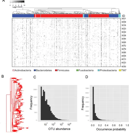
Fig. 2A shows the OTU count table for the 98 COMBO samples. From the count table, we
can see five major characteristics of the OTU data.
First, the OTU count data are high-dimensional. The number of OTUs usually exceeds the
number of samples. For example, at the species level (97% similarity), the COMBO data
have 17,303 OTUs. Even consolidating the species-level OTUs into genera, we still have
127 genera. Variable selection becomes important for analysis of high-dimensional data.
Second, the OTUs are related by a phylogenetic tree (Fig. 2AB). The phylogenetic tree
provides an important prior knowledge on the evolutionary relationship among OTUs. It
can be useful in at least three ways:
The tree is informative to define a biologically meaningful distance measure. Consider a
scenario, where we have two microbial communities with each having a unique set of OTUs.
If the two sets of OTUs are closely related and interleaved on the tree, the two microbial
communities share much of their evolutionary history and intuitively their distance should
be small. On the other extreme, if these two sets of OTUs are located on different clades
of the tree, each community has their own unique evolutionary history and their distance
distinguish between these two situations.
The tree can guide OTU selection. Closely related OTUs are genetically more similar and
they are expected to have similar biological functions and respond to the environmental
perturbation in a similar way. They have a natural tendency to be selected together. This
is an important prior knowledge that we should exploit in OTU selection.
The tree also provides a hierarchical grouping of the OTUs. Environmental factor tends to
affect one/several OTU lineages (OTUs that share a common ancestor) of different depths.
Typically, microbiome data analysis is often performed at different taxonomic levels (genus,
family, order, class, phylum). However, the taxonomic classification is usually arbitrary.
Using the grouping structure implied by the OTU tree is more natural.
Third, the OTU counts are overdispersed, meaning that the variance of the counts is much
larger than what would be predicted by assuming a common multinomial model. Fig. 4B
shows that the counts generated by the multinomial model lacks variation compared to
the real counts (Fig. 4A). Models allowing for overdispersion should be used to model the
counts.
Fourth, the distribution of OTU abundance is very skewed (Fig. 2C). The majority of
the OTUs have very low abundance with a large fraction being singletons (OTUs with
only one sequence). The OTU count data are usually dominated by a small number of
highly abundant OTUs. However, it is hard to say the low-abundance OTUs are not
important. Statistical methods that place too much weight on the abundant lineages may
miss important findings if the biologically important change occurs in less abundant lineages.
Finally, the distribution of the OTU occurrence probability is also skewed (Fig. 2D). Only
a few OTUs are shared across samples, and the rest are seen in only a small percentage of
the samples. This results in excessive 0’s in the OTU data. Excessive 0’s may be a result
of count overdispersion or due to other mechanisms. Adequately modeling excessive 0’s is
The original OTU data are high-dimensional count data on the phylogenetic tree. Since the
sequencing depth varies from sample to sample, the count data are usually normalized into
proportions. As a way of further summarization, the data can be represented as pairwise
distances between the samples, which can be thought as projecting the original data into
lower dimensional space. In principle, we can develop statistical methods on any level of
data summarization (counts, proportions and distances). However, from counts to distances,
a large amount of information is lost, and the statistical power will be reduced accordingly.
For proportion data, the variability associated with multinomial sampling is lost. Pairwise
distances only capture certain features of the data.
In summary, the statistical challenges of OTU data analysis include incorporation of the
OTU phylogenetic tree information, treatment of rare OTUs, modeling high-dimensional
counts with overdispersion and excessive 0’s, modeling high-dimensional composition/proportion
data, and defining distance measures that capture a variety of microbiome differences.
1.5. Organization of the dissertation
The rest of the dissertation is organized as follows. Chapter 2 presents a distance based
method for testing the association between overall microbiome composition and
environ-mental/biological covariates. A generalized UniFrac distance (GUniFrac), which extends
the classic UniFrac distances (Lozupone and Knight, 2005; Lozupone et al., 2007), is
de-fined between two microbiomes. The power of GUniFrac based test is compared to other
UniFrac variants using simulations as well as the COMBO data set and an oropharyngeal
microbiome data set(Charlsonet al., 2010).
When there are a large number of covariates, variable selection becomes important.
Chap-ter 3 and ChapChap-ter 4 provide two methods for selecting the most important covariates under
different frameworks. Chapter 3 proposes a method for structure-constrained sparse
canon-ical correlation analysis (ssCCA), taking into account the phylogenetic relationship among
as an exploratory analysis method. It takes OTU proportion data and outputs the most
correlated OTUs and covariates. An efficient coordinate descent algorithm is implemented
to obtain the ssCCA solution. The performance of ssCCA is compared to sparse CCA using
simulations and the COMBO data set.
ssCCA takes the OTU proportion data, which does not consider the variation associated
with multinomial sampling, and the result does not show detailed individual OTU-covariate
associations. To deal with these limitations, a sparse Dirichlet-multinomial regression
(SDMR) method, which links the OTU counts to covariates under a regression setting,
is proposed. SDMR takes the OTU count data and outputs all identified associations. The
OTU counts are modeled using Dirichlet-multinomial distribution to account for
overdis-persion, and a sparse group l1 penalty function is imposed to achieve desired sparsity. A
block-coordinate descent algorithm is implemented to obtain the maximum penalized
like-lihood estimate. The selection performance of SDMR is also evaluated using simulations
and the COMBO data set in comparison to other possible models.
Chapter 5 concludes the dissertation with future research directions. Chapter 2-4 are
Extract DNA and PCR amplify with barcoded primer
Pool amplicons
Pyrosequence amplicons using 454’s
GS FLX instrument
Quality control, assign sequences to samples using barcode and denoise
align to reference alignment (e.g., using PYNAST), infer phylogeny (FastTree)
Species level OTUs can be summarized into higher taxonomic levels (e.g. genus)
Cluster sequences into OTUs (97% level), Assign a taxonomic
lineage to each OTU by RDP classifier
Figure 2: Characteristics of OTU data illustrated using the COMBO data. (A) The heatmap shows the OTU counts for the 98 COMBO samples. Rows represent samples and columns correspond to OTUs. These OTUs are related by a phylogenetic tree colored by phyla. The gray scale indicates the level of abundance on a log scale with white meaning zero counts (see legend). (B) The phylogenetic tree of OTUs. (C) The histogram shows the
OTU abundance distribution. The OTU abundance (x-axis) is on the log scale. (D) The
CHAPTER 2 : Associating Microbiome Composition with Environmental
Covariates using Generalized UniFrac Distance
In this chapter, we propose a new distance for characterizing the difference between two
microbial communities(microbiomes). Distance based statistical tests have been applied to
test the association of microbiome composition with environmental/biological covariates.
The unweighted and weighted UniFrac distances are the most widely used distance
mea-sures. However, these two measures assign too much weight either to rare lineages or to
highly abundant lineages, which can lead to loss of power when the important composition
change occurs in moderately abundant lineages. We develop generalized UniFrac distance
that extends weighted and unweighted UniFrac distances for detecting a much wider range
of biologically relevant changes. We evaluate the use of generalized UniFrac distance in
associating microbiome composition with environmental covariates using extensive Monte
Carlo simulations. Our results show that tests using the unweighted and weighted UniFrac
distances are less powerful in detecting abundance change in moderately abundant lineages.
In contrast, the generalized UniFrac distance is most powerful in detecting such changes, yet
it retains nearly all its power for detecting rare or highly abundant lineages. The generalized
UniFrac distance also has an overall better power than the joint use of unweighted/weighted
UniFracs distances. Application to two real microbiome data sets have demonstrated gains
in power in testing the associations between human microbiomes and dietary intake and
smoking. An R package has been developed for generalized UniFrac distance and is available
athttp://cran.r-project.org/web/packages/GUniFrac.
2.1. Introduction
Understanding the compositional differences of microbial communities is essential in
micro-bial ecology. With the development of next generation sequencing technologies, microbiome
composition can now be determined by direct DNA sequencing without the need for
body sites, ranging from skin (Griceet al., 2009) to gut (Qinet al., 2010; Arumugamet al.,
2011; Muegge et al., 2011; Wu et al., 2011a) and respiratory tract (Charlson et al., 2010,
2011; Sze et al., 2012). Important insights have been gained from analysis of large-scale
human microbiome data, including the discovery of enterotypes (Arumugam et al., 2011)
and discovery of the link between diet and these enterotypes (Wuet al., 2011a).
Two recurring themes in human microbiome studies are to identify potential environmental
factors that are associated with microbiome composition, and to define the relationship
between microbiome features and biological or clinical outcomes. The goal is to provide a
better understanding of the factors that shape our microbiome and, potentially, contribute
to the development of new therapeutic strategies to modulate the microbiome
composi-tion (Spor et al., 2011; Virgin and Todd, 2011) and affect the human health. Testing the
association of microbiome composition with potential environmental factors using OTU
abundances directly is difficult due to high dimensionality, non-normality and phylogenetic
structure of the OTU data. Instead, distance based non-parametric test, in which a
dis-tance measure is defined between any two microbiome samples, is usually used to achieve
this goal (Fukuyama et al., 2012; Evans and Matsen, 2012; Kuczynski et al., 2010a; Wu
et al., 2011a, 2010; Charlson et al., 2010). The power of the distance based test depends
on a proper choice of a distance measure. Numerous distance measures have been proposed
to compare microbial communities (Kuczynski et al., 2010b; Swenson, 2011). Phylogenetic
distance measures, which account for the evolutionary relationship among species, provide
far more power because they exploit the degree of divergence between different sequences.
Among these, the UniFrac distances are the most popular ones (Lozupone and Knight,
2005; Lozupone et al., 2007). There are two versions of UniFrac distances: an unweighted
UniFrac distance that considers only species presence and absence information and counts
the fraction of branch length unique to either community, and a weighted UniFrac distance
that uses species abundance information and weights the branch length with abundance
difference. Unweighted UniFrac distance is most efficient in detecting abundance change
the sequencing machine may not be able to pick it up and it will appear absent in the
final data set. On the other hand, weighted UniFrac distance is most sensitive to detect
change in abundant lineages since it uses absolute abundance difference in its definition.
However, Unweighted/weighted UniFrac distances may not be very powerful in detecting
change in moderately abundant lineages. Recently, a variance adjusted weighted UniFrac
distance (VAW-UniFrac), which moderates the branch proportion difference by its variance,
was developed to account for the fact that weighted UniFrac distance does not consider the
variation of the weights under random sampling (Chang et al., 2011). VAW-UniFrac was
shown to increase the power over weighted UniFrac distance for detecting the difference
between two microbial communities.
In this chapter, we introduce generalized UniFrac distance that unifies weighted UniFrac
and unweighted UniFrac distances. The new generalized UniFrac distance covers a series
of distances ranging from weighted to unweighted UniFrac by adjusting the weight on the
branches. The generalized UniFrac distance is designed to provide a robust and powerful
tool for detecting a wider range of biologically relevant changes in microbiome composition.
We conduct extensive Monte Carlo simulation studies under various conditions to evaluate
their power in detecting environmental influence on microbiome composition using
PER-MANOVA (McArdle, 2001), a distance based non-parametric test. Although each distance
in the series can perform the best in certain scenarios, none has optimal performance under
all conditions considered. However, analyses based on the generalized UniFrac distance are
shown to be more robust and has overall the best performances across a range of possible
scenarios. We demonstrate the power gain of using this distance in detecting the microbiome
differences by analysis of two real human gut microbiome data sets related to linking human
gut microbiome composition to long-term diet (Wuet al., 2011a) and testing oropharyngeal
2.2. Generalized UniFrac distance between two microbial communities
Consider two microbiome communities Aand B and suppose that we have a rooted
phylo-genetic tree withn branches. Letbi be the length of the branch iand pAi , pBi are the taxa
proportions descending from the branchifor communityAandB, respectively. The unique
fraction metric, or UniFrac, measures the phylogenetic distance between sets of taxa in a
phylogenetic tree as the fraction of the branch length of the tree that leads to descendants
from either one environment or the other, but not both. The original definition refers to
unweighted UniFrac (Lozupone and Knight, 2005), which is mathematically defined as
dU =
n X
i=1
bi
I(pAi >0)−I(pBi >0)
Pn
i=1bi
,
whereI(.) is the indicator function and only presence/absence of species of branchi,I(pA
i >
0) andI(pBi >0), are used in the definition. The distance definitiondU completely ignores
the taxa abundance information. In contrast, the (normalized) weighted UniFrac distance
(Lozuponeet al., 2007) weights the branch length with abundance difference and is defined
as
dW =
n X
i=1
bi
pAi −pBi
n X
i=1
bi(pAi +pBi )
.
Note that dW can not be reduced to dU even if we convert abundance data into
pres-ence/absence data. Also note thatdW uses the absolute proportion difference pAi −pBi
in
its formulation. The consequence of using the absolute difference is that the value ofdW is
determined mainly by branches with large proportions and is less sensitive to the abundance
changes on the branches with small proportions. To attenuate the weight on branches with
large proportions, we may instead use the relative differencepAi −pBi
in the formulation. We denote this distance measure as
d(0) =
n X
i=1
bi
pAi −pBi pA
i +pBi
n X
i=1
bi
,
wherePn
i=1bi in the denominator is the normalizing factor so that d(0)∈[0,1]. Now if we
dichotomize the abundance data using the indication function I(.), d(0) is reduced to dU.
Sod(0) can be seen as the “weighted version” ofdU. Using the relative differences, we place
equal emphasis on every branch and the distance is not dominated by the branches with
large proportions, since the relative difference does not depend on the magnitude ofpAi , pBi .
However, the low-abundance branches may be more noisy and the relative difference may
amplify such noises. To strike a balance between relative difference and absolute difference,
we weight the branch length both by the relative difference and its importance indicated
by the branch proportion. We propose the following generalized UniFrac distance
d(α)=
n X
i=1
bi(pAi +pBi )α
pAi −pBi pA
i +pBi
n X
i=1
bi(pAi +pBi )α
,
whereα∈[0,1] controls the contribution from high-abundance branches, andPn
i=1bi(pAi +
pBi )α is the normalizing factor so that d(α) ∈ [0,1]. Branches with zero proportions for
both communities will not be included in the calculation. Asα changes from 0 to 1, more
emphasis is placed on high-abundance branches. Whenα= 1,d(α)is reduced todW. When
α= 0, we get d(0) defined above.
Therefore, by varying α from 1 to 0 , we achieve a series of distances ranging from dW to
We are particularly interested ind(0.5), the distance in the middle of the distance series
d(0.5) =
n X
i=1
bi q
pAi +pBi
pAi −pBi pAi +pBi
n X
i=1
bi q
pAi +pBi .
We also compare dW, d(0.5), d(0) and dU to VAW-UniFrac distance dV AW, which is defined
as:
dV AW =
n X
i=1
bi
pAi −pBi
m(m−mi) n
X
i=1
bi
pAi +pBi m(m−mi)
,
where mi is the total number of sequences from both communities on the ith branch, and
m is total number of sequences.
2.3. Statistical test based on UniFrac distances
We study the power of generalized UniFrac distance using the distance-based non-parametric
test for association of microbiome composition with environmental covariates. Suppose we
have a set of m environmental covariates. We assume that we have collected microbiome
data and them-dimensional covariates dataX onnsamples. We apply the PERMANOVA
procedure (McArdle, 2001) (Permutational Multivariate Analysis of Variance Using
Dis-tance Matrices, “adonis” function from R package “vegan”), which partitions the disDis-tance
matrix among sources of variation, fits linear models to distance matrices and uses a
per-mutation test with pseudo-F ratios to obtain thep-values. The pseudo-F statistic is defined
as:
F = tr(HGH)/(m−1)
tr[(I−H)G(I−H)]/(n−m),
where tr(.) is the trace function of a matrix, H = X(XTX)−1XT is the hat (projection)
matrix of the design matrix X, G is Gower’s centered matrix and n, m is the number
communityiand j, and denoteA= (aij) = (−12d2ij). The Gower’s matrix is defined as
G= (I−11
0
n )A(I−
110
n ),
where1 is a vector of 1’s.
SincedU and dW reflect the abundance change in either rare lineages or abundant lineages,
combining dU and dW may potentially increase the overall power. Instead of applying
Bonferroni correction to the p values from separate PERMANOVA tests usingdU ordW to
control the family-wise type I error rate, a more powerful approach is to take the maximum
of pseudo-F statistics fordU anddW as a new test statistic. The significance of the pseudo-F
statistics is assessed based on permutations.
2.4. Simulation studies
2.4.1. Simulation strategies
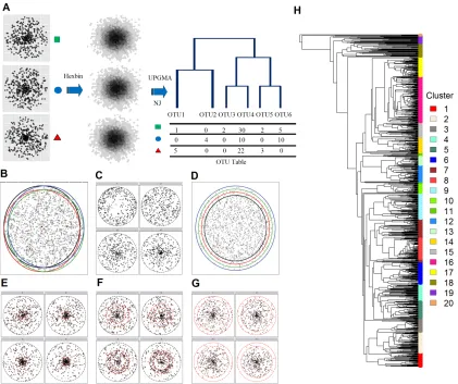
We use two simulation strategies to evaluate the power of the generalized UniFrac distance
under various conditions. The first strategy is a modification of the simulation method
proposed by Schloss (2008), where we draw points (16S rDNA sequences) from a 2D circle
with known densities (Fig. 3A). This strategy facilitates simulations of different community
characteristics such as species evenness and richness. The Euclidean distance between points
is analogous of the genetic distance between the sequences. The diameter of the circle
represents the maximum genetic divergence between any pair of sequences within a sample.
The area of the circle is proportional to the richness and the density distribution of the
circle is proportional to the evenness. By varying the centroid positions (o) and their radius
(r), it is possible to vary the fraction of shared membership and species richness within each
sample (Fig. 3B,D). By varying the point distribution on the circle (density proportional
to rα, where α controls the degree of evenness and α = 0.5 for uniformly distribution),
it is possible to change the species evenness (Fig. 3C). We also simulate scenarios where
by simulating the community with point mass concentrated at the circle center (r1.0) and
varying the point density in different regions of the 2D circle corresponding to abundant
lineages (0−0.2r from the center, Fig. 3E), moderately abundant lineages (0.4r−0.8r from
the center, Fig. 3F), and rare lineages (0.8r−1.0r from the center, Fig. 3G). We further
bin the sampled points into small hexagons as “OTU”s before calculating the UniFrac
distances (“hexbin” function from the R package “hexbin” ). The phylogenetic tree of
these “OTU”s is built using NJ algorithm (Neighbor Joining, “nj” function in R) and
rooted by midpoint rooting method. UniFrac distances are then calculated based on the
NJ tree and “OTU” abundances. Each replication consists of drawing 400 points from each
community, a bin size of 0.015 units to form “OTUs” (∼ 300 OTUs per sample), and the
maximum distance between any two points is 0.3 units (r= 0.15), corresponding to typical
phylum level divergence of 30% for 16S rRNA gene. These conditions allow us to simulate
the sampling intensity and biodiversity found within a typical 16S rRNA gene targeted
sequencing experiment (Schloss, 2008).
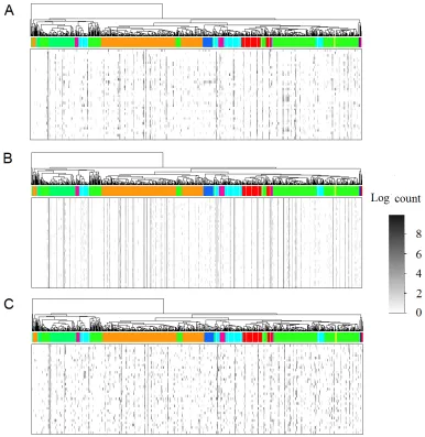
The second set of simulations utilizes a real oropharyngeal microbiome data set consisting of
60 samples and 856 OTUs from Charlsonet al.(2010) (Fig. 3H). A common way of modeling
multivariate count data is to use the multinomial model. However, the multinomial model
assumes fixed underlying proportions for each sample, which does not hold for real
micro-biome data due to high degree of heterogeneity among the samples. The real OTU count
distribution (Fig. 4A) exhibits more variance than expected from a multinomial model
(Fig. 4B). To realistically simulate the data, it is important to model extra-variation or
overdispersion of the OTU counts. This can be achieved by using the Dirichlet-multinomial
(DM) model (Mosimann, 1962), which assumes the underlying proportions of the
variableN is given as
P(N=n) =
n
n
k Y
j=1 nj
Y
r=1
{πj(1−θ) + (r−1)θ}
n Y
r=1
{1−θ+ (r−1)θ}
,
wheren=P
jnjis total count,kis the OTU number, and proportion meanπ= (π1, π2,· · · , πk)
and dispersionθare parameters. Whenθ= 0, it is reduced to multinomial model. We
esti-mate the DM parametersπ, θ using maximum likelihood method (“dirmult” function from
R package “dirmult”). We then generate OTU counts using the DM model with the
esti-mated parameters and 1,000 counts per sample. Fig. 4C shows an OTU heatmap generated
by the DM model, in which the overdispersion is similar to that of the real data. To study
the power of UniFrac variants for identifying potential environmental factors, we let the
abundance of a certain OTU cluster change in response to environment. We use UPGMA
tree of OTUs (“hclust” function in R) based on the OTU distance matrix calculated under
the K80 nucleotide substitution model (Felsenstein, 2003), and partition the 856 OTUs into
20 clusters using Partitioning Around Medoids (PAM) (“pam” function from R package
“cluster”) based on patristic distances (the length of the shortest path linking two OTUs
on the tree). These OTU clusters are highlighted in different colors in Fig. 3H.
We call the first strategy 2D circle based simulation and the second tree based simulation.
For power calculation, we use 2,000 replications.
2.4.2. Comparison of the power of different UniFrac variants using 2D circle based
simu-lations
We use PERMANOVA to test for environmental effects and compare the power ofdW, d(0.5), d(0),
dU and dV AW . Specifically, we simulate two environmental conditions (e.g. smoking vs
non-smoking) under which we draw 10 samples each. We then vary the degree of community
UniFrac distance. We investigate six scenarios, where the environmental factor affects the
community membership, species evenness, species richness, most abundant lineages,
mod-erately abundant lineages, and rare lineages respectively (Fig. 3B-G). For each scenario,
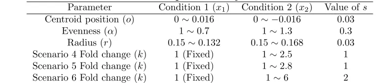
we vary one community characteristic (Table 1).
Suppose x1 and x2 are the mean values of the community characteristic for condition 1
and 2. We simulate 10 communities for each condition with community characteristic
value xij ∼ Uniform(xj −s, xj +s) for i = 1· · ·10 and j = 1,2, where s controls the
variation within each condition. Each community is sampled once. Initially, we letx1=x2
(no difference) and then increase the difference between x1 and x2 to simulate stronger
environmental effects. PERMANOVA is then performed on the distance matrices and the
power curve is created over a grid of 10 using type I error α = 0.05. Fig. 5 shows the
power curves for different UniFrac distances under the six scenarios considered. When the
environmental factor has no effect (x1 =x2), PERMANOVA controls the type I error at
the nominal level of 0.05 for all five UniFrac distances. As the environmental effects become
stronger, all the distances have better power. When the environmental factor affects the
community membership or richness (Panel 1, 3), all the distances give a similar power and
their power curves are nearly identical. For the evenness change scenario (Panel 2), the
power ofdW andd(0.5) is very close and is more powerful thand(0) anddU. dW is the most
powerful for detecting change in most abundant lineages (Panel 4) but is much less powerful
for change in rare lineages (Panel 6). dU shows an opposite trend: it is the most powerful
for detecting change in rare lineages (Panel 6) but has almost no power for change in most
abundant lineages (Panel 4). In contrast, d(0.5) is the most powerful for detecting change
in moderately abundant lineages (Panel 5). They are also the most robust among the
distances investigated: its power is close to the best UniFrac distance under all scenarios.
The performance of d(0) lies between d(0.5) and dU, and is also very robust. Finally, the
performance ofdV AW is almost identical tod(0.5) under this simulation setting.
sample). To study the effect of bin size, we compare the power curves of UniFrac distances
using a smaller bin size of 0.01 (∼700 OTUs per sample) or a larger bin size of 0.03 (∼80
OTUs per sample). The bin size does not change the general conclusion (Appendix Fig.
A1). To study the effect of tree construction methods, we also construct the phylogenetic
tree using UPGMA. The general conclusions still hold (Appendix Fig. A2).
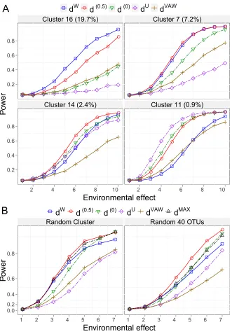
2.4.3. Comparison of the power of different UniFrac variants using tree based simulations
We also compare the power of different UniFrac distances for detecting environmental effects
using tree based simulations that mimic the oropharyngeal microbiome data (see Section
2.5.2 for details). The phylogenetic tree of the 856 OTUs is partitioned into 20 clusters (Fig.
3H). The mean OTU proportions and the dispersion parameter are estimated from the real
data by fitting a Dirichlet-multinomial (DM) model. We assume that the environmental
factor causes an increase of the abundance of a particular OTU cluster. Specifically, suppose
that the proportion of the ith OTU cluster under condition 1 is pi. For condition 2, the
proportion ofith OTU cluster is increased bykfold wherekvaries from 1 (no difference) to
1/√pi (strong effect) on a grid of 10. The proportion vector is re-normalized to sum to 1.
Next, 10 samples are simulated for each condition with their OTU counts generated by the
DM model with the corresponding proportion vector and the common dispersion parameter.
As expected, the five UniFrac distances differ in their power for detecting environmental
effects for the 20 OTU clusters tested. Except for d(0), all the UniFrac distances have
their best-performance scenarios. dW, d(0.5), dU and dV AW achieve the highest power in
7, 6, 3 and 1 cases respectively. For the remaining 3 cases, dW and d(0.5) are equally the
most powerful (Appendix Fig. A3). The results are consistent with the 2D-circle based
simulation: dW is most powerful for detecting the environmental effects on most abundant
lineages, d(0.5) for moderately abundant lineages and dU for rare lineages. In contrast,
performance of the test withd(0) and dV AW is generally betweendU and d(0.5). The power
of dW and dU has a reciprocal relationship and neither of them is as robust as d(0.5). Fig.
cluster decreases from 19.7% to 0.9%, dW becomes less powerful and the power ofdU has
the opposite trend.
In the simulations presented above, the power is calculated assuming we know the cluster
effected. Since the cluster affected can be abundant or rare, we randomly choose an affected
OTU cluster in each replication and calculate the power over 2,000 replications. We also
report the power for the test combiningdW anddU by taking the maximum of their
pseudo-F statistics. We denote this method asdM AX. Fig. 6B (left plot) demonstrates thatdU and
dV AW have the lowest overall power than the other distances, andd(0.5)anddM AX have the
best power indicating combining dU and dW can increase power. In contrast, d(0)and dW
are in between and as the environmental effect becomes stronger,d(0) becomes as powerful
as d(0.5) and dM AX. Lastly we assume that the environmental factor affects a random set
of 40 OTUs from the phylogenetic tree instead of a random OTU cluster. At this extreme,
where phylogenetic relationship is no longer important, d(0.5) has even higher power than
the other distances, followed by d(0), dM AX, dW, dU and dV AW (see Fig. 6B, right plot).
Overall, d(0.5) has a better power than any other UniFrac distances including the one that
combines dW and dU.
2.5. Application to real data analysis
2.5.1. Results from analysis of a data set linking long-term diet to gut microbiome
compo-sition
Diet strongly affects the human health, partly by modulating gut microbiome composition.
Wu et al. (2011a) studied the long term diet effect on the human gut microbiome, where
the diet information was converted into a vector of micro-nutrient intakes. A cross-sectional
analysis of 98 healthy volunteers were enrolled in this study. Diet information was collected
using food frequency questionnaire (FFQ). The questionnaires were converted to intake
amounts of 214 micro-nutrients. Nutrient intake was further normalized using the residual
of the 16S rRNA gene was sequenced by 454/Roche GS FLX Titanium system. The 16S
pyrosequences were denoised (Quince et al., 2009) prior to taxonomic assignment yielding
an average of 9,265±3,864(SD) reads per sample. The denoised sequences were then
analyzed by the QIIME pipeline (Caporasoet al., 2010b) with the default parameter setting.
The OTU table contains 3068 OTUs after discarding the singleton OTUs. We use the
phylogenetic tree generated by QIIME (FastTree algorithm, Priceet al. 2009) to construct
the UniFrac distances. One objective of the study is to identify nutrients that have a
significant impact on the gut microbiome composition. We use PERMANOVA to test
for association of microbiome composition with nutrient intake based on different UniFrac
distance matrices. We compared(0.5) withdU,dW, their combinationdM AX anddV AW. We
plot the number of selected nutrients against different p-value cutoffs to create a ROC-like
curve (Fig. 7). Clearly the curve for d(0.5) is above all the other four curves. Wilcoxon
signed-rank tests show that d(0.5) results in smaller p-values than other distances (p <
0.05), indicating thatd(0.5) is most powerful in selecting the relevant microbiome-associated
nutrients. Using dW ordU only could miss important associations. Power of dV AW is the
second best. Interestingly, dM AX, the joint use of dW and dU, does not increase the power
overdW, indicating most associations can be recovered by dW alone.
2.5.2. Results from analysis of an oropharyngeal microbiome data set smokers and
non-smokers
Cigarette smokers have an increased risk of multiple diseases, including upper respiratory
tract infections. Previous studies had linked smoking to specific respiratory tract bacteria
but the consequences of smoking for global airway microbial community composition had
not been fully clarified. Charlsonet al. investigated the smoking effect on the oropharyngeal
and nasopharyngeal bacterial communities using 454 pyrosequencing of 16S sequence tags
Charlsonet al. (2010). Specifically, a total of 291 swab samples from the right and left
na-sopharynx and oropharynx of 29 smoking and 33 nonsmoking healthy asymptomatic adults
individually barcoded primer set and subject to multiplexed pryosequencing by 454/Roche
GS FLX Titanium system. The pyrosequences were denoised (Quinceet al., 2009) prior to
taxonomic assignment and yielded an average of 1,335±603(SD) reads per airway
sam-ple. The denoised sequences were then analyzed using the QIIME pipeline (Caporasoet al.,
2010b) with default parameter setting. We use the left oropharyngeal samples in this study.
After removing two samples with read number less than 500 and discarding singleton OTUs,
we finally have an OTU table of 60 samples (28 smokers vs 32 nonsmokers) and 856 OTUs.
The phylogenetic tree produced by QIIME was used to construct the distances.
We test the smoking effect on the oropharyngeal microbial community composition by
applying PERMANOVA (10,000 permutations). All the five UniFrac distances achieve
sta-tistical significance atα= 0.05 level, indicating smoking alters the community composition.
However, test using d(0.5) produces the smallest p-value of 0.006, followed by 0.008 from
d(0). The p-values based on dW,dU anddV AW are 0.012, 0.019 and 0.043 respectively. We
also perform a principle coordinate analysis on the distance matrices, and plot the samples
on the first two principle coordinates (Fig. 8). d(0.5) separates the samples better than
the other three distance measures. This indicates that smoking might affect not only the
predominant lineages but also these less abundant lineages in the oropharyngeal microbial
community. We then performed Wilcox rank-sum test or Fisher’s exact test to select the
differential OTUs. At α = 0.05 level, we identify 32 OTUs (Appendix Table A1). These
OTUs belong to genera Prevotella (8), Lachnospiraceae (5), Veillonella (3), Streptococcus
(2), Fusobacterium (2), Treponema (2), Neisseria (1), Haemophilus (1), Megasphaera (1),
Dialister (1), Moryella (1), Erysipelotrichaceae (1) and four genera from Actinobacteria.
Most of the selected OTUs are moderately abundant or rare, so we expect d(0.5) and d(0)
to have better power.
Finally, we study the effect of tree constructing methods on generalized UniFrac distance.
Besides using the tree from QIIME, we also construct the phylogenetic tree by NJ,
distance matrix generated by the R function “dist.dna” from the “ape” package
(pair-wise.deletion=T) under the K80 nucleotide substitution model Felsenstein (2003). The
parsimony and maximum likelihood methods are implemented using the DNAPARS and
DNAML program with default parameter setting in PHYLIP 3.69. All the unrooted trees
are rooted using midpoint rooting method. We observe that different tree constructing
methods produce similar results (Appendix Fig. A4).
2.6. Discussion
Microbiome data are multivariate count data in its original form and are statistically
challenging to analyze due to their high dimensionality, phylogenetic constraints among
species/OTUs, overdispersion and excessive zeros. To circumvent the difficulty, the data
are often summarized in the form of distance matrix. Testing association of microbiome
composition with environmental covariates is performed using the distance matrix. We
have demonstrated in simulations that the weighted and unweighted UniFrac impose large
weight either to abundant lineages or to rare lineages, they can be underpowered in
detect-ing change in moderately abundant lineages. Since microbiome composition change could
occur in any lineages, our generalized UniFrac distance, which unifies the weighted and
unweighted UniFrac in a common framework enable us to detect a much wider range of
biologically relevant changes. Our simulation studies have clearly demonstrated that the
generalized UniFrac distanced(0.5) is more robust than dW ordU, and its performances are
in general comparable to the best UniFrac distances among the scenarios we considered.
In addition, the generalized UniFrac distance is very robust to tree constructing
meth-ods. We suggest the use of d(0.5) for testing association of microbiome composition with
environmental covariates to avoid missing important findings.
Both weighted and unweighted UniFrac distances are sensitive to sampling depth (Lozupone
et al., 2010). Inflated distances at lower sampling depth are caused by sampling variation
especially for these rare lineages. The generalized UniFrac distance is also sensitive to
For the gut microbiome data set, we found a sequencing depth of∼1000 reads is sufficient to
stabilize the generalized UniFrac distance. To overcome potential adverse effects of uneven
sampling, rarefaction is usually employed to subsample the samples to the same depth.
When the sampling depth varies greatly across the samples, rarefaction will throw away
a significant portion of the 16S reads and increase the sampling variation artificially. We
found that rarefaction is not necessary, at least, in the context of testing the association of
the microbiome composition with covariates (Fig. 10).
The VAW-UniFrac (Chang et al., 2011) also up-weights the differences on less abundant
lineages by adjusting the variance of the weights. If we assume the number of reads from
the two communities are the same and divide the weights ind(0.5) by
q
(2−pAi −pBi ), then
d(0.5) becomes VAW-UniFrac. Usually the majority of the branches have low proportions,
so
q
(2−pAi −pBi ) for majority of the branches are similar (∼√2). This accounts for the
similarity ofd(0.5) anddV AW in the 2D circle based simulations. When the phylogenetic tree
is constructed based on the OTUs of multiple samples (>2), the lowest common ancestor
(LCA) of any two communities is not necessarily the same as the root of the whole tree.
This is frequently seen in real data, where some samples occupy only a subtree. These
common branches between the LCA and the root are not included in the calculation of
VAW-UniFrac distance due to division by 0 for these branches. Ignoring these common
branches will inflate the distance. In contrast, d(0.5) does not have this limitation. This
accounts for the superiority ofd(0.5) overdV AW in tree-based simulation as well as in real
data analysis.
The power of UniFrac variants can also be compared in the context of testing whether two
microbial communities differ significantly as in (Schloss, 2008; Changet al., 2011). Instead
of comparing power for detecting the difference between two communities, we focus our
evaluations on the performance of UniFrac distances for associating microbiome
composi-tion to environmental covariates by collecting multiple independent samples. The racomposi-tional
to detect differences due to sources that we are not interested in (random noises), such as
the individual-to-individual variability, day-to-day variability, sampling location variability
or even technical variability (e.g. sample preparation). Multiple samples from a population
coupled with multivariate statistical methods such as the distance based PERMANOVA,
provide powerful design and analysis methods to overcome these potential random noises
(Lozupone et al., 2010). As more and more large-scale microbiome data sets are being
collected, we expect that our generalized UniFrac distance can help to identify important
covariates that are associated with the microbiomes that could be missed using the
com-monly used UniFrac distances. In addition to identifying environmental covariates that
may be determinants of microbiome composition, our approach would be equally suited
to identifying microbiome features associated with biological or clinical outcomes, which is