On the ﬂuctuation spectra of seismo-electromagnetic phenomena

(1)

www.nat-hazards-earth-syst-sci.net/11/301/2011/ doi:10.5194/nhess-11-301-2011

and Earth

System Sciences

On the fluctuation spectra of seismo-electromagnetic phenomena

M. Hayakawa

University of Electro-Communications (UEC), Advanced Wireless Communications Research Center, 1-5-1 Chofugaoka, Chofu Tokyo 182-8585, Japan

UEC, Research Station on Seismo Electromagnetics, Chofu Tokyo, Japan

Information Systems Inc., Earthquake Analysis Laboratory, 4-8-15 Minami-Aoyama, Minato Tokyo 107-0062, Japan Received: 7 October 2010 – Revised: 26 October 2010 – Accepted: 29 October 2010 – Published: 3 February 2011

Abstract. In order to increase the credibility on the presence of electromagnetic phenomena associated with an earthquake, we have suggested the importance of the modulation (or fluctuation) seen in the time-series data of any seismogenic effects. This paper reviews the fluctuation spectra of seismogenic phenomena in order to indicate the modulation mechanisms in the lithosphere, atmosphere and ionosphere/magnetosphere. Especially, the effect of Earth’s tides in the lithosphere and the modulation in the atmosphere (acoustic and atmospheric gravity waves) are discussed and this kind of fluctuation spectra would further provide essential information on the generation mechanisms of different seismogenic effects. Furthermore, the important role of the slope of fluctuation spectra is suggested in order to investigate the self-organized criticality before the lithospheric rupture and its associated effects in different regions such as the ionosphere.

1 Introduction

There has been a substantial accumulation of convincing evidence of electromagnetic phenomena in association with earthquakes (EQs) in the last decades (e.g., Hayakawa, 1999, 2009a; Hayakawa and Molchanov, 2002; Molchanov and Hayakawa, 2008). We can indicate a few examples of those seismo-electromagnetic effects which might be used for the short-term EQ prediction: (1) ULF (Ultra-low frequency) electromagnetic emissions from the lithosphere (e.g., Fraser-Smith et al., 1990; Kopytenko et al., 1993; Hayakawa et al., 1996), and (2) seismo-ionospheric perturbations

Correspondence to: M. Hayakawa (hayakawa@whistler.ee.uec.ac.jp)

in the lower ionosphere (D/E regions) (e.g., Hayakawa, 2007) and in the upper ionosphere (F layer or so) (e.g., Pulinets and Boyarchuk, 2004; Liu et al., 2006). A recent monograph edited by Hayakawa (2009a) includes several review papers on different seismogenic aspects containing recent progress, present knowledge, and future subjects to do (Fraser-Smith, 2009; Biagi, 2009; Kopytenko et al., 2009; Hayakawa, 2009b, c; Liu, 2009; Parrot, 2009; Pulinets, 2009; Molchanov, 2009; Freund, 2009).

(2)

302 M. Hayakawa: Fluctuation spectra of seismo-electromagnetic phenomena

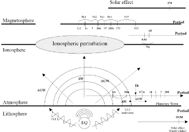
Fig. 1. Illustration on what kinds of possible modulations are expected in different regions (lithosphere, atmosphere, ionosphere/magnetosphere and the Sun). Possible periods of modulations are indicated. Also, two important seismo-electromagnetic effects are shown: (1) ULF lithospheric emissions and (2) seismo-ionospheric perturbations.

2 General idea on the possible modulations in the lithosphere, atmosphere and ionosphere/magnetosphere

As is already mentioned in the Introduction, two major seismogenic phenomena are our greatest concern; (1) seis-mogenic ULF emissions and (2) ionospheric perturbations. In Fig. 1, those two major seismogenic effects are indicated, which seem to be very promising candidates for short-term EQ prediction.

Figure 1 summarizes possible candidates of inducing modulations in different areas, which can be expected to be observed in seismo-electromagnetic effects. The most significant lithospheric effect is the modulation by Earth’s tide with the synodic period of 29.5 days because Tanaka et al. (2004) and Sue (2009) have recently found the significance of Earth’s tides in triggering EQs. While there are several possible modulation agencies present in the atmosphere: from the shorter period to the longer, AWs (acoustic waves) (in the period from 1 min to 10 min), AGWs (atmospheric gravity waves, period =∼10 min to a few hours), and PWs (planetary waves, period∼days). These are the typical characteristic oscillations in the atmosphere (e.g., Beer, 1974), which can be excited by different kinds of ground surface perturbations including meteorological, seismic influences, etc. PWs are long

waves influenced by the curvature of the earth and its rotation, which propagate mainly horizontally and provide a meteorologically useful theory for the description of the pressure distribution associated with moving wave-like high-(or low-)pressure system (Beer, 1974). In addition to this planetary wave with large scale, there exist other atmospheric oscillations with smaller temporal and spatial scales; AGW and AW. AWs tend to propagate vertically upwards, while AGWs generally propagate upward but obliquely (e.g., Beer, 1974). When we go upwards, as in Fig. 1, there exists a clear modulation of one day and half a day oscillation known as Sq (solar quiet variation) in the ionosphere (Nagata and Tohmatsu, 1973). Then, the oscillations known as geomagnetic pulsations (e.g., Pc1∼Pc5) (e.g., Saito, 1969) are the magnetospheric modulation effect expected to be observed in seismo-electromagnetic effects. Further, the recurrence periodicity of geomagnetic activity in close relation to the rotation of the Sun (with a period of 27 days) is a possible agent in the magnetosphere.

3 Lithospheric modulation

(3)

Fig. 2. An example of possible lithospheric modulation due to Earth’s tides (synodic period of 29.5 days) appeared in the ULF emissions for

the 2000 Izu EQ swarm. Adapted from Hayakawa et al. (2009).

clearly seen only for huge EQs. Tanaka (2006) has provided some more evidence that the EQs occurred near the epicentre of the 2004 Sumatra EQ were affected by the Earth’s tides for a period of 10 years before the main shock. EQs are fundamentally a mechanical phenomenon, no matter whether it is macroscopic or microscopic. Of course, the microscopic effect (such as microfracturing) of EQs seems to result in the precursory seismo-electromagnetic effect, one typical example being seismogenic ULF emissions (e.g., Hayakawa et al., 2007; Fraser-Smith, 2009; Kopytenko et al., 2009). So it is anticipated that such an effect of the Earth’s tides (with the period of 29.5 days) would also be noticed even in the seismo-electromagnetic data, but only in the case of large EQs. Hayakawa et al. (2009) have investigated the effect of the Earth’s tides in different seismo-electromagnetic phenomena.

Figure 2 presents one example of such an effect of the Earth’s tides in the detection of seismogenic ULF emissions which is adapted from Hayakawa et al. (2009). This is the result on the temporal evolution of the 3rd principal component of the ULF emission on the basis of principal component analysis (using 3 station data) (Gotoh et al., 2002) for the 2000 Izu islands EQ swarm. The principal component analysis by Gotoh et al. (2002) indicates that the first principal (strongest) component is highly likely to be the space effect of geomagnetic variations and the second component is found to be noise due to the man-made activity. And, the last (weakest) component is a residue, which can be considered seismogenic if it exists. We notice in Fig. 2 a clear modulation with the period of about one month close to the synodic period of 29.5 days (one to three months before the EQ), which is reasonably considered as the effect of the Earth’s tides. Such a modulation is also detected for some other ULF emission events.

As compared with the lithospheric ULF emissions, such an effect of the Earth’s tides in subionosphseric VLF/LF data (or ionospheric perturbations) is found not to be conspicuous, but still existing (Hayakawa et al., 2009). This poor effect in the ionosphere is probably due to the presence of the atmosphere between the lithosphere of the initial agent and the ionosphere.

4 Atmospheric modulation

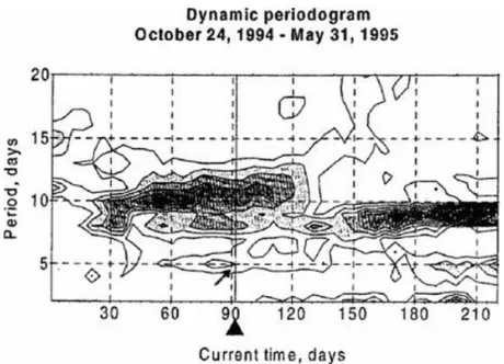
Our pioneering paper by Hayakawa et al. (1996) indicated the clear identification of ionospheric perturbations for the disastrous Kobe EQ by means of subionospheric propagation from the Omega VLF transmitter at Tsushima in Kyushu to the observing station at Inubo. That is, we discovered significant shifts in terminator time (morning and evening), mainly before the EQ. Because of the original nature of terminator times, one datum is obtained for one day, so that we can monitor the modulation only of the order of days. Figure 3 is one of such examples taken from Molchanov and Hayakawa (1998). One can find the precursory enhancement of the fluctuation wavelets with periods of 5 days and

∼10 days, which are considered to be the period of PWs. The paper by Molchanov and Hayakawa (1998) indicated, on the basis of 11 EQ events during 13 years, that only when the modulation with a period of either a few days, 5 days or

∼10 days is enhanced before the EQ, we can identify the occurrence of seismo-ionospheric perturbations.

(4)

Fig. 3. An example of modulation of PWs in the subionospheric

VLF/LF data (after Molchanov and Hayakawa, 1998). EQ day is given as a black triangle on the abscissa. The ordinate means the modulation period and the intensity is given in darkness.

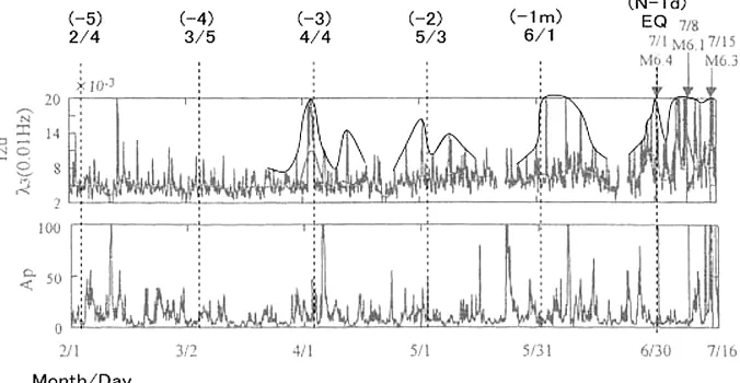
before an EQ. Later extensive works have been done on this AGW effect (Rozhnoi et al., 2004, 2007; Muto et al., 2009a, b; Kasahara et al., 2010). One example in Fig. 4 is taken from Muto et al. (2009b), which clearly indicates the conspicuous enhancement in AGW modulation just before a huge EQ (so-called Miyagi-oki EQ on 16 August 2005 with magnitude of 7.2 and depth of 36 km). The area enclosed by a red box is corresponding to the period around the Miyagi-oki EQ and the bottom panel indicates the AGW modulation index normalized by its standard deviation (σ). The second panel refers to the trend (nighttime average amplitude) and the top, nighttime fluctuation (the details of these two parameters are seen in Muto et al., 2009b and Kasahara et al., 2010). Together with the significant decrease in trend and the significant enhancement in nighttime fluctuation, we have found a very significant increase in the AGW fluctuation at least for this EQ.

Recently, Kasahara et al. (2010) have made the first statis-tical analysis on the AGW modulation in the subionospheric VLF/LF data. Based on different propagation paths in and around Japan and also during a long-enough period of nine years, Kasahara et al. (2010) have made the first statistical analysis on the AGW effect in subionospheric VLF/LF amplitude data. Figure 5 is their final result, in which the abscissa indicates the day before the EQ (–) and the day after the EQ (+) (EQ day is day 0) and the ordinate shows the AGW modulation index normalized by its standard deviation. Some explanation of AGW modulation index is necessary here. We make a residuedA(t ) as A(t )−< A(t ) >, where A(t ) is the VLF/LF amplitude at a time t on a particular day and< A(t ) >is the mean amplitude at the same timet averaged over±15 days around the current day. The nighttime dA(t ) is subjected to FFT analysis to obtain the fluctuation spectrum S(f ) on the current day.

< S(f ) >is the mean value of S(f ) averaged again over

±15 days around the current day and then we estimate dS(f )=S(f )−< S(f ) >. The range of AGW is from 10 min to 100 min and we pay attention only to the parts ofdS(f ) >0, then integratingdS(f ) >0 over the relevant frequency range (this is the AGW modulation index). The details are found in Muto (2009b) and Kasahara et al. (2010). The red line in Fig. 5 refers to shallow (depth<40 km) EQs, while the blue line refers to deep (depth≥40 km) EQs. This is the result of superimposed epoch analysis, in which the number of events for shallow EQs is 54 and that for deep EQs is 45. A glance at Fig. 5 indicates that the AGW index for deep EQs remains just around zero during the whole period, which means that there is no activated effect in AGW modulation in the lower ionosphere in the case of deep EQs. This is reasonably acceptable. On the other hand, the corresponding result for shallow EQs (in red) is found to be completely different from that for deep EQs. Undoubtedly we can recognize a very significant activation of AGW fluctuation 12 days before the EQ. This value of 12 days is not so important, but anyway several days before the EQ. Though the significance level of this enhancement does not exceed the conventional 2σ criterion, it notably amounts to about 1.5σlevel, which seems significant.

Here we have to comment on the relationship between the AW and AGW modulations (Hayakawa, 2009b). As shown in Fig. 3, we notice a visible delay between the climax of EQ process (moment of the main shock) and the time of wavelet centre. This delay is several days. However, the matter is that upward transport of PW energy is very slow and the expected transport time from the bottom of atmosphere to the lower ionosphere is more than 20–30 days. So, we need to suppose that such PW oscillations are coupled with a faster carrier wave, for example, AGW. We consider, for simplicity, that some amplitude-modulated AGWs as a carrier propagate upward with PW signal modulation. If we assume that there exists some nonlinearity in the ionosphere, we can easily expect the modulations of PWs in subionospheric VLF/LF data as in Fig. 3.

5 Ionospheric, magnetospheric and solar modulations

As is shown in Fig. 1, there are some modulations expected in the ionosphere (Sq effects) and expected modulations by means of geomagnetic pulsations (Pc1 to Pc5). However, there have been no such studies on the modulations in seismo-electromagnetic phenomena including ULF emissions and subionospheric VLF/LF data.

(5)

Fig. 4. Temporal evolutions of three physical parameters (nighttime fluctuation (NF), top; trend (nighttime average amplitude), middle; and

AGW modulation index, bottom) during four months including the date of Miyagi-oki EQ on 16 August 2005 (Muto et al., 2009b). All of the three quantities are normalized by their corresponding standard deviations (σ) (during –30 to –1 day of the current day). The downward red bars in each panel indicate the times of EQs with length indicating the magnitude. In the red box you can find two red vertical bars and red means that all of three physical quantities satisfy their criteria, suggesting that these peaks are seismogenic as a precursor and an after-effect of the EQ. Gray zone means the period of no observation.

6 Slopes of fluctuation spectra

In the previous sections, a remarkable periodicity based on the physical process is expected to be observed and be really observed in any seismogenic data. This kind of periodicities can be easily obtained by the corresponding analysis of the frequency spectrum of the time series data. However, it might be possible that some other useful information (except the previous periodicities easily found) are embedded in any time-series data of different seismogenic physical data. For example, it is known that the self-organization process takes place before any significant rupture of such an EQ (Hayakawa and Ida, 2008). In order to extract this useful information, we need to adopt any particular signal processing.

Hayakawa et al. (1999) studied, for the first time, the frequency spectra of seismogenic ULF emissions, who found that the spectrum slope (which can be related to the fractal dimension) changes significantly before the 2003 Guam EQ. Later a lot of these fractal analyses have been applied to ULF emissions for different EQs (Smirnova et al., 2001, 2004; Gotoh et al., 2003, 2004; Eftaxias et al., 2004; Ida et al., 2005; Ida and Hayakawa, 2006). Here we present,

Fig. 5. The superimposed epoch analysis of the AGW modulation in

(6)

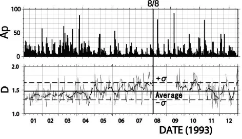
Fig. 6. Temporal evolution of mono-fractal dimension (D) during

one whole year of 1993 (bottom panel). The day of EQ is indicated by a vertical line with the notation of 8/8 (8 August). The upper panel indicates the geomagnetic activity expressed by Ap index. Daily D value is given in a thin line and the average value running over±15 days is given by a thick line. The average D value over the whole period is indicated by a horizontal line and the ±σ (σ: standard deviation over the whole period) lines are given in broken lines. After Ida and Hayakawa (2006) and Hayakawa and Ida (2008).

in Fig. 6, one example on the temporal evolution of mono-fractal dimension of ULF emissions for the 2003 Guam EQ (Ida and Hayakawa, 2006; Hayakawa and Ida, 2008). The bottom panel of Fig. 6 refers to the fractal dimension, which indicates a significant change in the fractal dimension (in this case, an increase) before the EQ. Further studies based on the multi-fractal analysis for the same EQ provided further information on the nonlinear self-organization process taking place in the lithosphere (Ida et al., 2006).

The slope of fluctuation spectra has been investigated by Molchanov et al. (2004) and Hobara et al. (2006), who have studied the fluctuation (in this case, spatial) distribution of the ionospheric plasma density and electric field turbulence observed on satellites in a form of k−b, where k is wave number and b is the slope or fractal index (Molchanov et al., 2004). They have concluded that though there may be some connection seen of the change in the fractal index to seismic effect, its effect is not so evident. The later study by Hobara et al. (2005) concludes that the effect of major seismic activities toward the ionospheric turbulence is not conclusive either for the refractive index or for the electric field power, but the mean value for the electric field power of bursts during seismic periods is significantly larger than that for non-seismic periods.

Recently, Imamura et al. (2010) have applied the fractal analysis to the local nighttime data of subionospheric LF propagation and the fractal dimension is estimated every day in the two distinct frequency ranges (AW and AGW). The data during several years are analysed for the propagation paths from the Japanese LF transmitter of JJY to Moshiri (Hokkaido) and to Kochi. They come to the conclusion that

when paying attention to the period around the EQ, they sometimes detect some significant increases in the fractal dimension in AW and/or AGW range. But, as in the case of previous satellite turbulence studies, the effect is not so strongly recognized.

7 Summary and conclusion

The fluctuation spectra of the different kinds of seismo-electromagnetic phenomena would provide essential in-formation on the modulation taken place at different regions (including the lithosphere, atmosphere, iono-sphere/magnetosphere and sun). The presence (or existence) of seismogenic electromagnetic phenomena, itself is still controversial, so that the modulation in the lithosphere and atmosphere would provide an additional confirmation that those effects are really seismogenic. Also, such modulation effects would be of extreme importance in obtaining further hints on the generation mechanisms of seismo-electromagnetic effects (ULF emissions, seismo-ionospheric perturbations, etc.). Apart from the previous conspicuous modulation periodicities, some other useful information embedded in the time-series data can be extracted from the slope of fluctuation spectra or fractal analysis, which would be useful for the study of self-organized criticality in the lithosphere and its effects even onto the ionosphere.

Acknowledgements. This work is, in part, supported by NICT (National Institute of Information and Comunications Technology), Japan. The author is grateful to the referees for their useful suggestions.

Edited by: C.-V. Meister

Reviewed by: P. F. Biagi and another anonymous referee

References

Beer, T.: Atmospheric Waves, Adam Hilger, London, 1974. Biagi, P. F.: Pre and post seismic disturbances revealed on the

geochemical data collected in Kamchatka (Russia) during the last 30 years, in: Electromagnetic Phenomena Associated with Earthquakes, edited by: Hayakawa, M., Transworld Research Network, Trivandrum, India, Chapter 4, 97–117, 2009.

Campbell, W. H.: Natural magnetic disturbance fields, not precursors, preceding the Lama Prieta earthquake, J. Geophys. Res., 114, A05307, doi:10.1029/2008JA013932, 2009.

Eftaxias, K., Frangos, P., Kapiris, P., Polygiannakis, J., Kopanas, J., Peratzakis, A., Skountzos, P., and Jaggard, D.: Review and a model of pre-seismic electromagnetic emissions in terms of fractal electrodynamics, Fractals, 12, 243–273, 2004.

(7)

Fraser-Smith, A. C., Bernardi, A., McGill, P. R., Ladd, M. E., Helliwell, R. A., and Villard Jr., O. G.: Low-frequency magnetic field measurements near the epicenter of the Ms7.1 Loma Prieta earthquake, Geophys. Res. Lett., 17, 1465–1468, 1990. Freund, F.: Stress-activated positive hole charge carriers in rocks

and the generation of pre-earthquake signals, in: Electro-magnetic Phenomena Associated with Earthquakes, edited by: Hayakawa, M., Transworld Research Network, Trivandrum, India, Chapter 3, 41–96, 2009.

Gotoh, K., Akinaga, Y., Hayakawa, M., and Hattori, K.: Principal component analysis of ULF geomagnetic data for Izu islands earthquakes in July 2000, J. Atmos. Electr., 22(1), 1–12, 2002. Gotoh, K., Hayakawa, M., and Smirnova, N.: Fractal analysis of

the ULF geomagnetic data obtained at Izu Peninsula, Japan in relation to the nearby earthquake swarm of June-August 2000, Nat. Hazards Earth Syst. Sci., 3, 229–236, doi:10.5194/nhess-3-229-2003, 2003.

Gotoh, K., Hayakawa, M., Smirnova, N. A., and Hattori, K.: Fractal analysis of seismogenic ULF emissions, Phys. Chem. Earth, 29, 419–424, 2004.

Hayakawa, M. (Ed.): Atmospheric and Ionospheric Electromag-netic Phenomena Associated with Earthquakes, TERRAPUB, Tokyo, 997 pp., 1999.

Hayakawa, M. (Ed.): Electromagnetic Phenomena Associated with Earthquakes, Transworld Research Network, Trivandrum, India, 279 pp., 2009a.

Hayakawa, M.: Seismogenic perturbation in the atmosphere, in: Electromagnetic Phenomena Associated with Earthquakes, edited by: Hayakawa M., Transworld Research Network, Trivandrum, India, Chapter 5, 119–136, 2009b.

Hayakawa, M.: Lower ionospheric perturbations associated with earthquakes, as detected by subionospheric VLF/LF radio signals, in: Electromagnetic Phenomena Associated with Earthquakes, edited by: Hayakawa M., Transworld Research Network, Trivandrum, India, Chapter 6, 137–186, 2009c. Hayakawa, M. and Ida, Y.: Fractal (mono- and multi-) analysis for

the ULF data during the 1993 Guam earthquake for the study of prefracture criticality, Current Development in Theory and Applications of Wavelets, 2(2), 159–174, 2008.

Hayakawa, M. and Molchanov, O. A. (Eds.): Seismo-Electromagnetics: Lithosphere-Atmosphere-Ionosphere Cou-pling, TERRAPUB, Tokyo, 477 pp., 2002.

Hayakawa, M., Kawate, R., Molchanov, O. A., and Yumoto, K.: Results of ultra-low-frequency magnetic field measurements during the Guam earthquake of 8 August 1993, Geophys. Res. Lett., 23, 241–244, 1996a.

Hayakawa, M., Molchanov, O. A., Ondoh, T., and Kawai, E.: The precursory signature effect of the Kobe earthquake on VLF subionospheric signals, J. Comm. Res. Lab. Tokyo, 43, 169–180, 1996b.

Hayakawa, M., Itoh, T., and Smirnova, N.: Fractal analysis of ULF geomagnetic data associated with the Guam earthquake on August 8, 1993, Geophys. Res. Lett., 26(18), 2797–2800, 1999. Hayakawa, M., Sue, Y., and Nakamura, T.: The effect of earth tides

as observed in seismo-electromagnetic precursory signals, Nat. Hazards Earth Syst. Sci., 9, 1733–1741, doi:10.5194/nhess-9-1733-2009, 2009.

Ida, Y. and Hayakawa, M.: Fractal analysis for the ULF data during the 1993 Guam earthquake to study prefracture criticality, Nonlin. Processes Geophys., 13, 409–412, doi:10.5194/npg-13-409-2006, 2006.

Ida, Y., Hayakawa, M., Adalev, A., and Gotoh, K.: Multifractal analysis for the ULF geomagnetic data during the 1993 Guam earthquake, Nonlin. Processes Geophys., 12, 157–162, doi:10.5194/npg-12-157-2005, 2005.

Kasahara, Y., Nakamura, T., Hobara, Y., Hayakawa, M., Rozhnoi, A., Solovieva, M., and Molchanov, O. A.: A statistical study on the AGW modulation in subionospheric VLF/LF propagation data and consideration of the generation mechanism of seismo-ionospheric perturbations, J. Atmos. Electr., 30(2), 103–112, 2010.

Kopytenko, Yu. A., Matiashvili, T. G., Veronov, P. M., and Molchanov, O. A.: Detection of ultra-low frequency emissions connected with the Spitak earthquake and its aftershock activity, based on geomagnetic pulsation data at Dusheti and Vardzia, Phys. Earth Planet. In., 77, 85–95, 1993.

Kopytenko, Yu. A., Ismagilov, V. S., and Nikitina, L. V.: Study of local anomalies of ULF magnetic disturbances before strong earthquakes and magnetic fields induced by tsunami, in: Electromagnetic Phenomena Associated with Earthquakes, edited by: Hayakawa, M., Transworld Research Network, Trivandrum, India, Chapter 2, 21–40, 2009.

Liu, J. Y.: Earthquake precursors observed in the ionospheric F-region, in: Electromagnetic Phenomena Associated with Earthquakes, edited by: Hayakawa M., Transworld Research Network, Trivandrum, India, Chapter 7, 187–204, 2009. Liu, J. Y., Chen, Y. I., and Chuo, Y. J.: A statistical study

of preearthquake ionosphere anomaly, J. Geophys. Res., 111, A05304, doi:10.1029/2005JA011333, 2006.

Miyaki, K., Hayakawa, M., and Molchanov, O. A.: The role of gravity waves in the lithosphere-ionosphere coupling, as revealed from the subionospheric LF propagation data, in: Seismo Electromagnetics: Lithosphere-Atmosphere-Ionosphere Coupling, edited by: Hayakawa, M. and Molchanov, O. A., TERRAPUB Tokyo, 229–232, 2002.

Molchanov, O. A.: Lithosphere-atmosphere-ionosphere coupling due to seismicity, in: Electromagnetic Phenomena Associated with Earthquakes, edited by: Hayakawa, M., Transworld Research Network, Trivandrum, India, Chapter 10, 255–279, 2009.

Molchanov, O. A. and Hayakawa, M.: Subionospheric VLF signal perturbations possibly related to earthquakes, J. Geophys. Res., 103(A8), 17489–17504, 1998.

Molchanov, O. A. and Hayakawa, M.: Seismo-Electromagnetics and Related Phenomena: History and Latest Results, TERRA-PUB Tokyo, 189 pp., 2008.

Molchanov, O. A., Hayakawa, M., and Miyaki, K.: VLF/LF sounding of the lower ionosphere to study the role of atmospheric oscillations in the lithosphere-ionosphere coupling, Advances in Polar Upper Atmosphere Research, 15, 146–158, 2001. Muto, F., Horie, T., Yoshida, M., Hayakawa M., Rozhnoi, A.,

(8)

Muto, F., Kasahara, Y., Hobara, Y., Hayakawa, M., Rozhnoi, A., Solovieva, M., and Molchanov, O. A.: Further study on the role of atmospheric gravity waves on the seismo-ionospheric perturbations as detected by subseismo-ionospheric VLF/LF propagation, Nat. Hazards Earth Syst. Sci., 9, 1111–1118, doi:10.5194/nhess-9-1111-2009, 2009b.

Nagata, T. and Tohmatsu, T.: Physics of the Upper Atmosphere, Shokabo Pub Comp., Tokyo, 1973 (in Japanese).

Parrot, M.: Anomalous seismic phenomena: View from space, in: Electromagnetic Phenomena Associated with Earthquakes, edited by: Hayakawa, M., Transworld Research Network, Trivandrum, India, Chapter 8, 205–234, 2009.

Pulinets, S.: Lithosphere-atmosphere-ionosphere coupling (LAIC) model, in: Electromagnetic Phenomena Associated with Earthquakes”, edited by: Hayakawa, M., Transworld Research Network, Trivandrum, India, Chapter 9, 235–254, 2009. Pulinets, S. A. and Boyarchuk, K.: Ionospheric Precursors of

Earthquakes, Springer, Berlin, 315 pp., 2004.

Rozhnoi, R., Solovieva, M. S., Molchanov, O. A., and Hayakawa, M.: Middle latitude LF (40 kHz) phase variations associated with earthquakes for quiet and disturbed geomagnetic conditions, Phys. Chem. Earth, 29, 589–598, 2004.

Rozhnoi, A., Solovieva, M., Molchanov, O., Biagi, P.-F., and Hayakawa, M.: Observation evidences of atmospheric Gravity Waves induced by seismic activity from analysis of subionospheric LF signal spectra, Nat. Hazards Earth Syst. Sci., 7, 625–628, doi:10.5194/nhess-7-625-2007, 2007.

Saito, T.: Geomagnetic pulsations, Space Sci. Rev., 10, 319–412, 1969.

Smirnova, N., Hayakawa, M., Gotoh, K., and Volobuev, D.: Scaling characteristics of ULF geomagnetic fields at the Guam seismoactive area and their dynamics in relation to the earthquake, Nat. Hazards Earth Syst. Sci., 1, 119–126, doi:10.5194/nhess-1-119-2001, 2001.

Smirnova, N., Hayakawa, M., and Gotoh, K.: Precursory behavior of fractal characteristics of the ULF electromagnetic fields in seismic active zones before strong earthquakes, Phys. Chem. Earth, 29, 445–451, 2004.

Sue, Y.: The effect of earth tides in triggering earthquake as clearly observed in some specific regions of Japan, J. Atmos. Electr., 29, 53–62, 2009.

Tanaka, S.: Tidal triggering of earthquakes precursory to the 2004 Mw=9.0 off Sumatra earthquake, Paper presented at 4th International Workshop on Statistical Seismology, Graduate Univ. for Advanced Study, Kanagawa, Japan, 9–13, 2006. Tanaka, S., Ohtake, M., and Sato, H.: Tidal triggering of

earthquakes in Japan related to the regional tectonic stress, Earth Planets Space, 56(5), 511–515, 2004.