Bayesian network learning for natural hazard analyses

(1)

Nat. Hazards Earth Syst. Sci., 14, 2605–2626, 2014 www.nat-hazards-earth-syst-sci.net/14/2605/2014/ doi:10.5194/nhess-14-2605-2014

Bayesian network learning for natural hazard analyses

K. Vogel1,*, C. Riggelsen2, O. Korup1, and F. Scherbaum1

1_{Institute of Earth and Environmental Sciences, University of Potsdam, Germany} 2_{Pivotal Software Inc., Palo Alto, USA}

*_{Invited contribution by K. Vogel, recipient of the Outstanding Student Poster (OSP) Award 2012.}

Correspondence to: K. Vogel ([email protected])

Received: 14 August 2013 – Published in Nat. Hazards Earth Syst. Sci. Discuss.: 22 October 2013 Revised: 26 June 2014 – Accepted: 19 August 2014 – Published: 29 September 2014

Abstract. Modern natural hazards research requires deal-ing with several uncertainties that arise from limited process knowledge, measurement errors, censored and incomplete observations, and the intrinsic randomness of the govern-ing processes. Nevertheless, deterministic analyses are still widely used in quantitative hazard assessments despite the pitfall of misestimating the hazard and any ensuing risks.

In this paper we show that Bayesian networks offer a flexi-ble framework for capturing and expressing a broad range of uncertainties encountered in natural hazard assessments. Al-though Bayesian networks are well studied in theory, their application to real-world data is far from straightforward, and requires specific tailoring and adaptation of existing al-gorithms. We offer suggestions as how to tackle frequently arising problems in this context and mainly concentrate on the handling of continuous variables, incomplete data sets, and the interaction of both. By way of three case studies from earthquake, flood, and landslide research, we demon-strate the method of data-driven Bayesian network learning, and showcase the flexibility, applicability, and benefits of this approach.

Our results offer fresh and partly counterintuitive in-sights into well-studied multivariate problems of earthquake-induced ground motion prediction, accurate flood damage quantification, and spatially explicit landslide prediction at the regional scale. In particular, we highlight how Bayesian networks help to express information flow and independence assumptions between candidate predictors. Such knowledge is pivotal in providing scientists and decision makers with well-informed strategies for selecting adequate predictor variables for quantitative natural hazard assessments.

1 Introduction

Natural hazards such as earthquakes, tsunamis, floods, land-slides, or volcanic eruptions have a wide range of differing causes, triggers, and consequences. Yet the art of predict-ing such hazards essentially addresses very similar issues in terms of model design: the underlying physical processes are often complex, while the number of influencing factors is large. The single and joint effects of the driving forces are not always fully understood, which introduces a potentially large degree of uncertainty into any quantitative analysis. Ad-ditionally, observations that form the basis for any inference are often sparse, inaccurate and incomplete, adding yet an-other layer of uncertainty. For example, Merz et al. (2013) point out the various sources of uncertainty (scarce data, poor understanding of the damaging process, etc.) in the context of flood damage assessments, while Berkes (2007) calls at-tention to the overall complexity of human–environment sys-tems, as well as the importance of understanding underlying uncertainties to improve resilience. Similarly, Bommer and Scherbaum (2005) discuss the importance of capturing un-certainties in seismic hazard analyses to balance between in-vestments in provisions of seismic resistance and possible consequences in the case of insufficient resistance.

Nevertheless, deterministic approaches are still widely used in natural hazards assessments. Such approaches rarely provide information on the uncertainty related to parame-ter estimates beyond the use of statistical measures of dis-persion such as standard deviations or standard errors about empirical means. However, uncertainty is a carrier of infor-mation to the same extent as a point estimate, and ignor-ing it or dismissignor-ing it as simply an error may entail grave consequences. Ignoring uncertainties in quantitative hazard

(2)

2606 K. Vogel et al.: Bayesian network learning for natural hazard analyses appraisals may have disastrous effects, since it often leads to

over- or underestimates of certain event magnitudes. Yet de-terministic approaches persist as the state of the art in many applications. For example, tsunami early warning systems evaluate pre-calculated synthetic databases and pick out the scenario that appears closest to a given situation in order to estimate its hazard (Blaser et al., 2011). Recently developed models for flood damage assessments use classification ap-proaches, where the event under consideration is assigned to its corresponding class, and the caused damage is estimated by taking the mean damage of all observed events belonging to the same class (Elmer et al., 2010). In seismic hazard anal-ysis the usage of regression-based ground motion models is common practice, restricting the model to the chosen func-tional form, which is defined based on physical constrains (Kuehn et al., 2009).

In this paper we consider Bayesian networks (BNs), which we argue are an intuitive, consistent, and rigorous way of quantifying uncertainties. Straub (2005) underlines the large potential of BNs for natural hazard assessments, herald-ing not only the ability of BNs to model various inter-dependences but also their intuitive format: the representa-tion of (in)dependences between the involved variables in a graphical network enables improved understandings and di-rect insights into the relationships and workings of a nat-ural hazard system. The conditional relationships between dependent variables are described by probabilities, from which not only the joint distribution of all variables but any conditional probability distribution of interest can be derived. BNs thus endorse quantitative analyses of specific hazard scenarios or process-response chains.

In recent years, BNs have been used in avalanche risk as-sessment (e.g., Grêt-Regamey and Straub, 2006), tsunami early warning (e.g., Blaser et al., 2009, 2011), earthquake risk management (e.g., Bayraktarli and Faber, 2011), proba-bilistic seismic hazard analysis (e.g., Kuehn et al., 2011), and earthquake-induced landslide susceptibility (e.g., Song et al., 2012). Aguilera et al. (2011) give an overview of applica-tions of BNs in the environmental sciences between 1990 and 2010, and conclude that the potential of BNs remains under-exploited in this field. This is partly because, even though BNs are well studied in theory, their application to real-world data is not straightforward. Handling of continuous variables and incomplete observations remains the key problem. This paper aims to overcome these challenges. Our objective is to briefly review the technique of learning BNs from data, and to suggest possible solutions to implementation prob-lems that derive from the uncertainties mentioned above. We use three examples of natural hazard assessments to discuss the demands of analyzing real-world data, and highlight the benefits of applying BNs in this regard.

In our first example (Sect. 3), we develop a seismic ground motion model based on a synthetic data set, which serves to showcase some typical BN properties. In this context we demonstrate a method to deal with continuous variables

with-Fig. 1. The figure shows the BN for the burglary example. The graph structure illustrates the dependence relations of the involved variables: The alarm can be triggered by a burglary or earthquake. An earthquake

might be reported in the radio newscast. The joint distribution of all variables can be decomposed into the

product of its conditionals accordingly:P(B, E, A, R) =P(B)P(E)P(A|B, E)P(R|E)

Fig. 2.Illustration of a parent set in a BN.XPa(i)is the parent set ofXi

(a) (b) (c)

Fig. 3. Working with continuous variables we have to make assumptions about the functional form of the probability distributions (gray), e.g.(a)exponential,(b)normal,(c)uniform. Thus we restrict the distributions to certain shapes that may not match reality. In contrast using a discrete multinomial distribution (black), each

continuous distribution can be approximated and we avoid prior restrictions on the shape. Rather the shape is

learned from the data by estimating the probability for each interval.

30

Figure 1. The figure shows the BN for the burglary exam-ple. The graph structure illustrates the dependence relations of the involved variables: the alarm can be triggered by a burg-lary or earthquake. An earthquake might be reported in the radio newscast. The joint distribution of all variables can be decomposed into the product of its conditionals accordingly:

P (B, E, A, R)=P (B) P (E) P (A|B, E) P (R|E).

out any prior assumptions on their distributional family. In Sect. 4 we use data that were collected after the 2002 and 2005/2006 floods in the Elbe and Danube catchments, Ger-many, to learn a BN for flood damage assessments. This ex-ample is emblematic of situations where data are incomplete, and requires a treatment of missing observations, which can be challenging in combination with continuous variables. Our final example in Sect. 5 deals with a regional landslide susceptibility model for Japan, where we investigate how the same set of potential predictors of slope stability may pro-duce nearly equally well performing, though structurally dif-ferent, BNs that reveal important and often overlooked vari-able interactions in landslide studies. This application further illustrates the model uncertainty related to BN learning.

2 Bayesian networks (BNs)

The probabilistic framework of BNs relies on the theorem formulated by Reverend Thomas Bayes (1702–1761), and expresses how to update probabilities in light of new evi-dence (McGrayne, 2011). By combining probability theory with graph theory, BNs depict probabilistic dependence re-lations in a graph: the nodes of the graph represent the con-sidered random variables, while (missing) edges between the nodes illustrate the conditional (in)dependences between the variables. Textbooks often refer to the burglary alarm sce-nario for a simple illustration of BNs (Pearl, 1998). In this example, the alarm of your home may not only be triggered by burglary but also by earthquakes. Moreover, earthquakes have a chance to be reported in the news. Figure 1 shows the dependence relations of these variables as captured by a BN. Now, imagine you get a call from your neighbor notifying you that the alarm went off. Supposing the alarm was trig-gered by burglary, you drive home. On your way home you hear the radio reporting a nearby earthquake. Even though burglaries and earthquakes may be assumed to occur inde-pendently, the radio announcement changes your belief in the burglary, as the earthquake “explains away” the alarm. BNs

(3)

K. Vogel et al.: Bayesian network learning for natural hazard analyses 2607

Table 1. Conditional probabilities in the burglary example, giv-ing the conditional probabilities for earthquake (e), burglary (b), alarm (a), and earthquake reported (r). The parameters that define the conditional distributions correspond for discrete variables to the conditional (point) probabilities. Note that the conditional probabil-ity values for no earthquake (e), no burglary (b), etc. can be derived from the fact that the conditionals sum up to 1.

θe=p(e) =0.001 θa|e,b=p(a|e, b) =0.98

θb=p(b) =0.01 θa|e,b=p(a|e, b) =0.95 θr|e=p(r|e) =0.95 θa|e,b=p(a|e, b) =0.95 θr|e=p(r|e) =0.001 θ_a|e,b=p(a|e, b) =0.03

offer a mathematically consistent framework to conduct and specify reasonings of such kind. A detailed introduction to BNs is provided in Koller and Friedman (2009) and Jensen and Nielsen (2001), while Fenton and Neil (2012) offers easy and intuitive access. In this paper we restrict ourselves to sev-eral key aspects of the BN formalism.

2.1 Properties and benefits

Applying BNs to natural hazard assessments, we define the specific variables of the hazard domain to be the nodes in a BN. In the following we denote this set of random variables asX= {X1, . . . , Xk}. The dependence relations between the

variables are encoded in the graph structure, generating a di-rected acyclic graph (DAG). The directions of the edges de-fine the flow of information, but do not necessarily indicate causality. As we shall see in subsection “Learned ground mo-tion model” of Sect. 3.2, it may prove beneficial to direct edges counterintuitively in order to fulfill regularization con-straints. The set of nodes from which edges are directed to a specific node,Xi, is called the parent set,XPa(i), ofXi (see

Fig. 2). Table 2 summarizes the notations used in this paper. Apart from the graph structure, a BN is defined by con-ditional probabilities that specify the dependence relations encoded in the graph structure. The conditional probability distribution for each variable,Xi, is given conditioned on its

parent set:p Xi|XPa(i)

. For simplification we restrict our-selves here to discrete variables for whichθis the set of con-ditional (point) probabilities for each combination of states for Xi andXPa(i):θ= {θxi|xPa(i)=p(xi|xPa(i))}. The condi-tional probabilities for the burglary BN example are given in Table 1. For continuous variables, the design of the param-eters depends on the family of distributions of the particular densitiesp(·|·).

Given the BN structure (DAG) and parameters (θ), it fol-lows from the axioms of probability theory that the joint dis-tribution of all variables can be factorized into a product of conditional distributions:

P (X|DAG,θ)= k

Y

i=1

p Xi|XPa(i)

. (1)

Fig. 1. The figure shows the BN for the burglary example. The graph structure illustrates the dependence relations of the involved variables: The alarm can be triggered by a burglary or earthquake. An earthquake might be reported in the radio newscast. The joint distribution of all variables can be decomposed into the product of its conditionals accordingly:P(B, E, A, R) =P(B)P(E)P(A|B, E)P(R|E)

(a) (b) (c)

Fig. 3. Working with continuous variables we have to make assumptions about the functional form of the probability distributions (gray), e.g.(a)exponential,(b)normal,(c)uniform. Thus we restrict the distributions to certain shapes that may not match reality. In contrast using a discrete multinomial distribution (black), each continuous distribution can be approximated and we avoid prior restrictions on the shape. Rather the shape is learned from the data by estimating the probability for each interval.

30

Figure 2. Illustration of a parent set in a BN.XPa(i)is the parent set ofXi.

Further, applying Bayes theorem, P (A|B)=P (A, B)

P (B) =

P (B|A) P (A)

P (B) , each conditional probability of interest can be

derived. In this way a BN is characterized by many attractive properties that we may profit from in a natural hazard setting, including the following properties:

– Property 1 – graphical representation: the interactions of the variables of the entire “system” are encoded in the DAG. The BN structure thus provides information about the underlying processes and the way various variables communicate and share “information” as it is propa-gated through the network.

– Property 2 – use prior knowledge: the intuitive inter-pretation of a BN makes it possible to define the BN based on prior knowledge; alternatively it may be learned from data, or even a combination of the two (cast as Bayesian statistical problem) by posing a prior BN and updating it based on observations (see below for details).

– Property 3 – identify relevant variables: by learning the BN from data we may identify the variables that are (according to the data) relevant; “islands” or isolated single unconnected nodes indicate potentially irrelevant variables.

– Property 4 – capture uncertainty: uncertainty can eas-ily be propagated between any nodes in the BN; we ef-fectively compute or estimate probability distributions rather than single-point estimates.

– Property 5 – allow for inference: instead of explicitly modeling the conditional distribution of a predefined target variable, the BN captures the joint distribution of all variables. Via inference, we can express any given or all conditional distribution(s) of interest, and reason in any direction (including forensic and inverse reason-ing): for example, for a given observed damage we may infer the likely intensity of the causing event. A detailed example for reasoning is given in Sect. 4.3.

(4)

2608 K. Vogel et al.: Bayesian network learning for natural hazard analyses

Table 2. Summary of notations used in this paper.

Notation Meaning

Xi a specific variable

xi a realization ofXi

X= {X1, . . . , Xk} set of the considered variables

XPa(i) parent set ofXi

x_Pa_(i) a realization of the parent set

X−Y all variables butY

DAG directed acyclic graph (graph structure)

p(Xi|XPa(i)) conditional probability of a variable conditioned on its parent set

θxi|xPa(i) parameter that defines the probability forxigivenxPa(i) θ=

n

θxi|xPa(i)

o

set of model parameters that defines the conditional distributions

2 random variable for the set of model parameters

BN: (DAG,θ) Bayesian network, defined by the pair of structure and parameters

d discrete/discretized data set that is used for BN learning

dc (partly) continuous data set that is used for BN learning

3 discretization that bins the original datadcintod

XMB(i) set of variables that form the Markov blanket ofXi(Sect. 4.2)

Ch(i) variable indices of the children ofXi(Sect. 4.2)

Note that inference in BNs is closed under restric-tion, marginalizarestric-tion, and combinarestric-tion, allowing for fast (close to immediate) and exact inference.

– Property 6 – use incomplete observations: during pre-dictive inference (i.e., computing a conditional distribu-tion), incomplete observations of data are not a problem for BNs. By virtue of the probability axioms, it merely impacts the overall uncertainty involved.

In the following we will refer to these properties 1–6 in order to clarify what is meant. For “real-life” modeling prob-lems, including those encountered in natural hazard analysis, adhering strictly to the BN formalism is often a challeng-ing task. Hence, the properties listed above may seem unduly theoretical. Yet many typical natural hazard problems can be formulated around BNs by taking advantage of these proper-ties. We take a data-driven stance and thus aim to learn BNs from collected observations.

2.2 Learning Bayesian networks

Data-based BN learning can be seen as an exercise in finding a BN which, according to the decomposition in Eq. (1), could have been “responsible for generating the data”. For this we traverse the space of BNs (Castelo and Kocka, 2003) look-ing for a candidate maximizlook-ing a fitness score that reflects the “usefulness” of the BN. This should however be done with careful consideration to the issues always arising in the context of model selection, i.e., over-fitting, generalization, etc. Several suggestions for BN fitness scoring are derived from different theoretical principles and ideas (Bouckaert, 1995). Most of them are based on the maximum likelihood estimation for different DAG structures according to Eq. (1).

In this paper we opt for a Bayesian approach to learn BNs (note that BNs are not necessarily to be interpreted from a Bayesian statistical perspective). Searching for the most probable BN, (DAG,θ), given the observed data,d, we aim to maximize the BN MAP (Bayesian network maximum a posteriori) score suggested by Riggelsen (2008):

P (DAG,2|d)

| {z }

posterior

∝P (d|DAG,2)

| {z }

likelihood

P (2,DAG)

| {z }

prior

. (2)

The likelihood term decomposes according to Eq. (1). The prior encodes our prior belief in certain BN structures and pa-rameters. This allows us to assign domain specific prior pref-erences to specific BNs before seeing the data (Property 2) and thus to compensate for sparse data, artifacts, bias, etc. In the following applications we use a non-informative prior, which nevertheless fulfills a significant function. Acting as a penalty term, the prior regularizes the DAG complexity and thus avoids over-fitting. Detailed descriptions for prior and likelihood term are given in Appendix A1 and Riggelsen (2008).

The following section illustrates the BN formalism “in ac-tion” and will also underscore some theoretical and practi-cal problems along with potential solutions in the context of BN learning. We will learn a ground motion model, which is used in probabilistic seismic hazard analysis, as a BN; the data are synthetically generated. Subsequently, we consider two other natural hazard assessments where we learn BNs from real-world data.

(5)

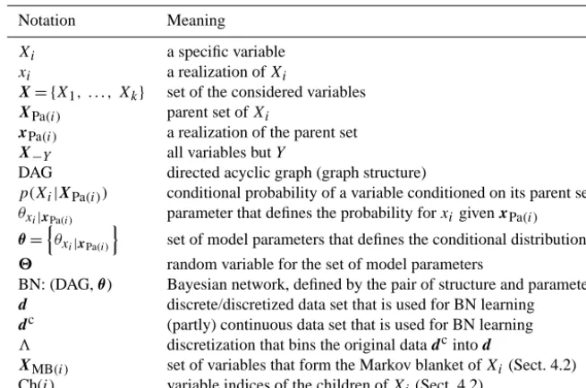
Table 3. Variables used in the ground motion model and the corresponding distributions used for the generation of the synthetic data set which is used for BN learning.

Xi Description Distribution[range]

Predictors

M Moment magnitude of the earthquake U[5,7.5]

R Source-to-site distance Exp[1 km,200 km]

SD Stress released during the earthquake Exp[0 bar,500 bar]

Q0 Attenuation of seismic wave amplitudes in deep layers Exp[0 s−1_,_{5000 s}−1_] κ0 Attenuation of seismic wave amplitudes near the surface Exp[0 s,0.1 s]

VS30 Average shear-wave velocity in the upper 30 m U[600 m s−1_,_{2800 m s}−1_]

Ground motion parameter

PGA Horizontal peak ground acceleration According to the stochastic model

(Boore, 2003)

3 Seismic hazard analysis: ground motion models When it comes to decision making on the design of high-risk facilities, the hazard arising from earthquakes is an impor-tant aspect. In probabilistic seismic hazard analysis (PSHA) we calculate the probability of exceeding a specified ground motion for a given site and time interval. One of the most crit-ical elements in PSHA, often carrying the largest amount of uncertainty, is the ground motion model. It describes the con-ditional probability of a ground motion parameter, Y, such as (horizontal) peak ground acceleration, given earthquake-and site-related predictor variables, X−Y. Ground motion

models are usually regression functions, where the func-tional form is derived from expert knowledge and the ground motion parameter is assumed to be lognormally distributed: lnY=f (X−Y)+, with ∼N(0, σ2). The definition of

the functional form off (·)is guided by physical model as-sumptions about the single and joint effects of the different parameters, but also contains some ad hoc elements (Kuehn et al., 2011). Using the Bayesian network approach there is no prior knowledge required per se, but if present it can be accounted for by encoding it in the prior term of Eq. (2). If no reliable prior knowledge is available, we work with a non-informative prior, and the learned graph structure pro-vides insight into the dependence structure of the variables and helps in gaining a better understanding of the underlying mechanism (Property 1). Modeling the joint distribution of all variables,X= {X−Y, Y}, the BN implicitly provides the

conditional distribution P (Y|X−Y, DAG,2), which gives

the probability of the ground motion parameter for specific event situations needed for the PSHA (Property 5).

3.1 The data

The event situation is described by the predictor variables

X−Y= {M, R,SD, Q0, κ0, VS30}, which are explained in Table 3. We generate a synthetic data set consisting of

Fig. 1. The figure shows the BN for the burglary example. The graph structure illustrates the dependence

relations of the involved variables: The alarm can be triggered by a burglary or earthquake. An earthquake

might be reported in the radio newscast. The joint distribution of all variables can be decomposed into the

product of its conditionals accordingly:P(B, E, A, R) =P(B)P(E)P(A|B, E)P(R|E)

(a) (b) (c)

Fig. 3. Working with continuous variables we have to make assumptions about the functional form of the

probability distributions (gray), e.g.(a)exponential,(b)normal,(c)uniform. Thus we restrict the distributions

to certain shapes that may not match reality. In contrast using a discrete multinomial distribution (black), each

continuous distribution can be approximated and we avoid prior restrictions on the shape. Rather the shape is

learned from the data by estimating the probability for each interval.

30

Figure 3. When working with continuous variables, we have to make assumptions about the functional form of the probability dis-tributions (gray), e.g., (a) exponential, (b) normal, and (c) uniform. Thus we restrict the distributions to certain shapes that may not match reality. In contrast, using a discrete multinomial distribution (black), each continuous distribution can be approximated and we avoid prior restrictions on the shape. Rather the shape is learned from the data by estimating the probability for each interval.

10 000 records. The ground motion parameter,Y, is the hor-izontal peak ground acceleration (PGA). It is generated by a so-called stochastic model which is described in detail by Boore (2003). The basic idea is to distort the shape of a ran-dom time series according to physical principles and thus to obtain a time series with properties that match the ground-motion characteristics. The predictor variables are either uni-form (U) or exponentially (Exp) distributed within a particu-lar interval (see Table 3).

The stochastic model does not have good analytical prop-erties, and its usage is non-trivial and time consuming. Hence, surrogate models, which describe the stochastic model in a more abstract sense (e.g., regressions), are used in PSHA instead. We show that BNs may be seen as a viable alternative to the classical regression approach. However, be-fore doing so, we need to touch upon some practical issues arising when learning BNs from continuous data.

For continuous variables we need to define the distri-butional family for the conditionals p(·|·) and thus make assumptions about the functional form of the distribu-tion. To avoid such assumptions and “let the data speak”, we discretize the continuous variables, thus allowing for

(6)

Fig. 4.

_:::::::::::

Representation

_::

of

_:::

For

_:::

the

_::::::::::

discretization

_:::::::

approach

_::::

each

multivariate continuous distribution

(a)

can be

_::

is

characterized

by a discrete distribution that captures the dependence relations

(b)

and a continuous uniform distribution over

each grid cell

(c)

: Assume

.

_:::

For

_::::::::::::

exemplification

_::::::

assume

cells corresponds to their probabilities

_:::::

(which

_:::

are

_::::::

defined

_::

by

_:::

θ

)

. A darker color means, that we expect more

realizations in this grid cell. Further we say, that within each grid cell the realizations are uniformly distributed,

as illustrated in

(c)

.

31

Figure 4. Representation of the dependency assumptions in the discretization approach: the dependency relations of the variables are captured by their discrete representations (gray-shaded area). A continuous variable,Xc_i, depends only on its discrete counterpart,

Xi.

completely data-driven and distribution-free learning (see Fig. 3). In the following subsection we describe an automatic discretization, which is part of the BN learning procedure and takes the dependences between the single variables into ac-count. However, the automatic discretization does not neces-sarily result in a resolution that matches the requirements for prediction purposes or decision support. To increase the po-tential accuracy of predictions, we approximate, once the net-work structure is learned, the continuous conditionals with

mixtures of truncated exponentials (MTE), as suggested by

Moral et al. (2001). More on this follows in Sect. 3.3.

3.2 Automatic discretization for structure learning

The range of existing discretization procedures differs in their course of action (supervised vs. unsupervised, global vs. local, top-down vs. bottom-up, direct vs. incremental, etc.), their speed and their accuracy. Liu et al. (2002) pro-vide a systematic study of different discretization techniques, while Hoyt (2008) concentrates on their usage in the context with BN learning. The choice of a proper discretization tech-nique is anything but trivial as the different approaches result in different levels of information loss. For example, a dis-cretization conducted as a pre-processing step to BN learning does not account for the interplay of the variables and often misses information hidden in the data. To keep the informa-tion loss small, we use a multivariate discretizainforma-tion approach that takes the BN structure into account. The discretization is defined by a set of interval boundary points for all vari-ables, forming a grid. All data points of the original contin-uous (or partly contincontin-uous) data set,dc, that lie in the same grid cell, correspond to the same value in the discretized data set, d. In a multivariate approach, the “optimal” discretiza-tion, denoted by3, depends on the structure of the BN and the observed data,dc. Similar to Sect. 2.2, we again cast the problem in a Bayesian framework searching for the combin-ation of (DAG,θ,3) that has the highest posterior probabil-ity given the data,

Fig. 4._:::::::::::Representation_::of_:::the_::::::::dependency_::::::::::assumptions_::in_::the_::::::::::discretization_::::::::approach:_:::The_:::::::::dependency_:::::::relations

:

of_:::the_:::::::variables_:::are_:::::::captured_::by_::::their_::::::discrete_:::::::::::representations_:::::(gray_:::::shaded_:::::area)._::A_::::::::continuous_:::::::variable,_::::Xc i,

::::::

depends_::::only_::on_::its_::::::discrete_:::::::::counterpart,_:::Xi.

Fig. 5.A_:::For_:::the_::::::::::discretization_:::::::approach_::::eachmultivariate continuous distribution(a)can be_::ischaracterized by a discrete distribution that captures the dependence relations(b)and a continuous uniform distribution over

each grid cell(c): Assume._:::For_::::::::::::exemplification_::::::assumewe consider two dependent, continuous variablesXc 1 andX_2.c _(a)_{shows a possible realization of a corresponding sample. According to Monti and Cooper (1998)} we now assume, that we can find a discretization, such that the resulting discretized variablesX1andX2

capture the dependence relation betweenXc

1andX2. This is illustrated byc (b), where the shading of the grid cells corresponds to their probabilities_:::::(which_:::are_::::::defined_::by_:::θ). A darker color means, that we expect more realizations in this grid cell. Further we say, that within each grid cell the realizations are uniformly distributed,

as illustrated in(c).

31

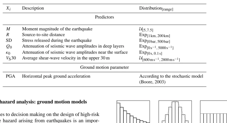
Figure 5. For the discretization approach each multivariate contin-uous distribution (a) is characterized by a discrete distribution that captures the dependence relations (b) and a continuous uniform dis-tribution over each grid cell (c). For exemplification assume we con-sider two dependent, continuous variables:Xc₁andXc₂. (a) shows a possible realization of a corresponding sample. According to Monti and Cooper (1998) we now assume that we can find a discretization, such that the resulting discretized variablesX1andX2capture the

dependence relation betweenXc₁andX₂c. This is illustrated by (b), where the shading of the grid cells corresponds to their probabilities (which are defined byθ). A darker color means that we expect more realizations in this grid cell. Further, we say that, within each grid cell, the realizations are uniformly distributed, as illustrated in (c).

P DAG,2, 3|dc

| {z }

posterior

∝P dc|DAG,2, 3

| {z }

likelihood

P (DAG,2, 3)

| {z }

prior

.(3)

Let us consider the likelihood term: expanding on an idea by Monti and Cooper (1998), we assume that all communica-tion/flow of information between the variables can be cap-tured by their discrete representations (see Fig. 4) and is de-fined by the parametersθ. Thus only the distribution of the discrete dataddepends on the network structure, while the distribution of the continuous datadc is, for givend, inde-pendent of the DAG (see Figs. 4 and 5). Consequently the likelihood for observingdc _{(for a given discretization,} net-work structure and parameters) can be written as

P dc|DAG,2, 3=P dc|d, 3P (d|DAG,2, 3) (4) and Eq. (3) decomposes into

P DAG,2, 3|dc∝P dc|d, 3

| {z }

continuous data

P (d|DAG,2, 3)

| {z }

likelihood (discrete) P (DAG,2, 3)

| {z }

prior .

(7)

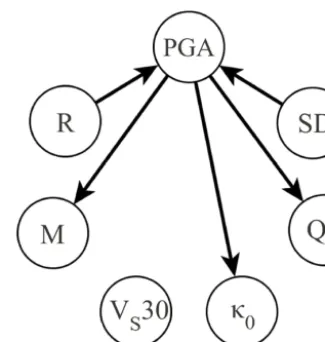
Figure 6. Theoretic BN for the ground motion model. It captures the known dependences of the data-generating model.

The likelihood (discrete) term is now defined as for the sep-arate BN learning for discrete data (Sect. 2.2), and we use a non-informative prior again. For the continuous data, we as-sume that all continuous observations within the same inter-val defined by 3 have the same probability (Fig. 5). More information about the score definition can be found in the Appendix A1, and technical details are given in Vogel et al. (2012, 2013). In the following we discuss the BN and dis-cretization learned from the synthetic seismic data set. Learned ground motion model

Since we generated the data ourselves, we know which (in)dependences the involved variables should adhere to; this is expected to be reflected in the BN DAG we learn from the synthetic data (Property 1, 3). Due to data construction, the predictor variablesM,R, SD,Q0,κ0, andVS30 are indepen-dent of each other and PGA depends on the predictors. Fig-ure 6 shows the dependence structFig-ure of the variables. The converging edges at PGA indicate that the predictors become conditionally dependent for a given PGA. This means that, for a given PGA, they carry information about each other; for example, for an observed large PGA value, a small stress drop indicates a close distance to the earthquake. The knowl-edge about the dependence relations gives the opportunity to use the seismic hazard application for an inspection of the BN learning algorithm regarding the reconstruction of the de-pendences from the data, which is done in the following.

The network that we found to maximize P (DAG,2, 3|dc) for the 10 000 synthetic seismic data records is shown in Fig. 7. The corresponding dis-cretization that was found is plotted in Fig. 8, which shows the marginal distributions of the discretized variables. The learned BN differs from the original one, mainly due to regularization constraints as we will explain in the following: as mentioned in Sect. 2, the joint distribution

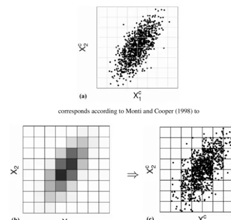
Figure 7. BN for the ground motion model learned from the gen-erated synthetic data. It captures the most dominant dependences. Less distinctive dependences are neglected for the sake of parameter reduction.

of all variables can be decomposed into the product of the conditionals according to the network structure (see Eq. 1). For discrete/discretized variables, the number of parameters needed for the definition ofp(Xi|XPa(i))in Eq. (1)

corre-sponds to the number of possible state combinations for (Xi, XPa(i)). Taking the learned discretization shown in Fig. 8,

the BN of the data-generating process (Fig. 6) is defined by 3858 parameters, 3840 needed alone for the description of p(PGA|M, R,SD, Q0, κ0, VS30). A determination of that many parameters from 10 000 records would lead to a strongly over-fitted model. Instead we learn a BN that compromises between model complexity and its ability to generate the original data. The BN learned under these requirements (Fig. 7) consists of only 387 parameters and still captures the most relevant dependences.

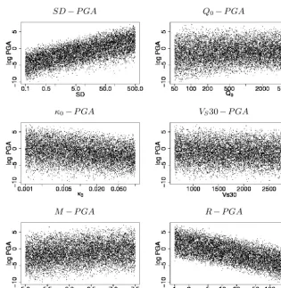
Figure 9 shows the ln PGA values of the data set plot-ted against the single predictors. A dependence on stress drop (SD) and distance (R) is clearly visible. These are also the two variables with remaining converging edges on PGA, revealing that, for a given PGA, SD contains information aboutRand vice versa. The dependences between PGA and the remaining predictors are much less distinctive, such that the conditional dependences between the predictors are neg-ligible and the edges can be reversed for the benefit of pa-rameter reduction. The connection toVS30 is neglected pletely, since its impact on PGA is of minor interest com-pared to the variation caused by the other predictors.

Note that the DAG of a BN actually maps the indepen-dences (not the depenindepen-dences) between the variables. This means that each (conditional) independence statement en-coded in the DAG must be true, while enen-coded dependence relations must not hold per se (see Fig. 10 for explanation). In turn this implies that each dependence holding for the data should be encoded in the DAG. The learning approach

(8)

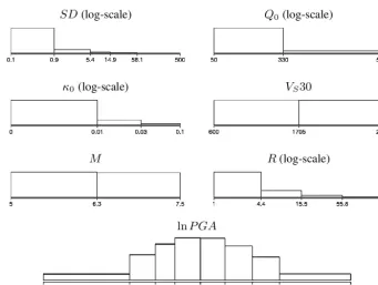
Fig. 8.Marginal distribution of the variables included in the ground motion model, discretized according to the

discretization learned for the BN in Fig. 7. The number of intervals per variable ranges from 2 to 8.

33

Figure 8. Marginal distribution of the variables included in the ground motion model, discretized according to the discretization learned for the BN in Fig. 7. The number of intervals per variable ranges from 2 to 8.

applied here fulfills the task quite well, detecting the rele-vant dependences, while keeping the model complexity at a moderate level.

The model complexity depends not only on the DAG but also on the discretization. A complex DAG will enforce a small number of intervals, and a large number of intervals will only be chosen for variables with a strong influence on other variables. This effect is also visible for the learned dis-cretization (Fig. 8). PGA is split into eight intervals, distance and stress drop into four and five, respectively, and the other variables consist of only two to three intervals.

3.3 Approximation of continuous distributions with mixtures of exponentials (MTEs)

A major purpose of the ground motion model is the predic-tion of the ground mopredic-tion (ln PGA) based on observapredic-tions of the predictors; hence, although the BN captures the joint distribution (Property 5) of all involved variables, the focus in this context is on a single variable. The accuracy of the prediction is limited by the resolution of the discretization learned for the variable. For the BN shown above, the dis-cretization of the target variable into eight intervals enables a quite precise approximation of the continuous distribution, but this is not the case per se. Complex network structures and smaller data sets used for BN learning lead to a coarser discretization of the variables. To enable precise estimates, we may search for alternative approximations of the (or at least some, in particular the primary variable(s) of interest)

continuous conditional distributions once the BN has been learned.

Moral et al. (2001) suggest using MTEs for this purpose, since they allow for the approximation of a variety of func-tional shapes with a limited number of parameters (Langseth and Nielsen, 2008) and they are closed under the opera-tions used for BN inference: restriction, combination, and marginalization (Langseth et al., 2009). The basic idea is to approximate conditional distributionsp(Xi|XPa(i))with a

combination/mixture of truncated exponential distributions. For this purpose the domain (Xi,XPa(i)) is partitioned into hypercubesD1, . . . , DL, and the density within each

hyper-cube,Dl, is defined such that it follows the form

p↓Dl Xi|XPa(i) ₌

a0+

J

X

j=1 ajebjXi

+cT

jXPa(i)_. ₍₅₎

The determination of the hypercubes and the number of ex-ponential terms in each hypercube as well as the estimation of the single parameters is done according to the maximum likelihood approach described in Langseth et al. (2010). In the following we show how the MTE approximation im-proves the BN prediction performance compared to the us-age of the discretized variables, and we compare the results to those from a regression approach.

Prediction performance

We conduct a 10-fold cross validation to evaluate the pre-diction performance of the BN compared to the regression

(9)

Fig. 9. The single figures show the dependences between the predictor variablesM, R,SD, Q0, κ0, VS30and the target variablelnPGA by plotting the data used to learn the BN for ground motion modeling.

Fig. 10. The graph structure of a BN dictates, how the joint distribution of all variables decomposes into a product of conditionals. Thus for a valid decomposition each independence assumption mapped into the BN

must hold. Usually this applies to a variety of graphs, i.e. the complete graph is always a valid independence

map as it does not make any independence assumption. (a)and(b)show two valid BN structures and the corresponding decompositions for the burglary example. The independence assumptions made in both BNs

hold, however(b)does not capture the independence between earthquakes and burglaries. An independence map that maps all independences(a)is called a perfect map, yet perfect maps do not exist for all applications. Besides, for parameter reduction it might be beneficial to work with an independence map that differs from the

perfect map.

34

Figure 9. The individual panels show the dependences between the predictor variablesM,R, SD,Q0,κ0, andVS30 and the target variable

ln PGA by plotting the data used to learn the BN for ground motion modeling.

approach: the complete data set is divided into 10 disjoint subsamples, of which one is defined as a test set in each trial while the others are used to learn the model (regression func-tion or BN). The funcfunc-tional form of the regression funcfunc-tion is determined by expert knowledge based on the description of the Fourier spectrum of seismic ground motion and follows the form

f (X−Y)=a0+a1M+a2M·ln SD+(a3+a4M) ln

q

a₅2+R2₊_a

6κR+a7VS30+a8ln SD, withκ=κ0+t∗,t∗=_Q₀R_V_sq andVsq=3.5 km s−1.

We compare the regression approach in terms of predic-tion performance to the BN with discretized variables and with MTE approximations. For this purpose we determine the conditional density distributions of ln PGA given the pre-dictor variables for each approach and consider how much probability it assigns to the real ln PGA value in each ob-servation. For the regression approach the conditional den-sity follows a normal distribution,N(f (X−Y), σ2), while it

is defined via the DAG and the parametersθ using the BN models. Table 4a shows for each test set the conditional den-sity value of the observed ln PGA averaged over the

individ-ual records. Another measure for the prediction performance is the mean squared error of the estimates for ln PGA (Ta-ble 4b). Here the point estimate for ln PGA is defined as the mean value of the conditional density. For example, in the regression model the estimate corresponds tof (x−Y).

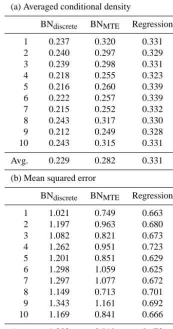
Even though the discretization of ln PGA is relative precise using the discrete BNs (eight intervals in each trial, except for the first trial, where ln PGA is split into seven intervals), the MTE approximation of the conditional distributions im-proves the prediction performance of the BN. Still, it does not entirely match the precision of the regression function. However, the prediction performances are on the same order of magnitude, and we must not forget that the success of the regression approach relies on the expert knowledge used to define its functional form, while the structure of the BN is learned in a completely data-driven manner. Further the re-gression approach profits in this example from the fact that the target variable (ln PGA) is normally distributed, which is not necessarily the case for other applications. Focusing on the prediction of the target variable the regression ap-proach also does not have the flexibility of the BN, which is designed to capture the joint distribution of all variables and thus allows for inference in all directions (Property 5),

(10)

Table 4. Results of a 10-fold cross validation to test the prediction performance of the BN (with discrete and MTE approximations of the conditional distributions) and the regression approach. (a) con-tains the calculated conditional densities for the observed ln PGA values averaged over each trial. (b) contains the mean squared error of the predicted ln PGA for each trial.

(a) Averaged conditional density

BNdiscrete BNMTE Regression

1 0.237 0.320 0.331

2 0.240 0.297 0.329

3 0.239 0.298 0.331

4 0.218 0.255 0.323

5 0.216 0.260 0.339

6 0.222 0.257 0.339

7 0.215 0.252 0.332

8 0.243 0.317 0.330

9 0.212 0.249 0.328

10 0.243 0.315 0.331

Avg. 0.229 0.282 0.331

(b) Mean squared error

BNdiscrete BNMTE Regression

1 1.021 0.749 0.663

2 1.197 0.963 0.680

3 1.082 0.821 0.673

4 1.262 0.951 0.723

5 1.201 0.851 0.629

6 1.298 1.059 0.625

7 1.297 1.077 0.672

8 1.149 0.713 0.701

9 1.343 1.161 0.692

10 1.169 0.841 0.666

Avg. 1.202 0.919 0.672

as exemplified in Sect. 4.3. Additional benefits of BNs, like their ability to make use of incomplete observations, will be revealed in the following sections, where we investigate real-world data.

4 Flood damage assessment

In the previous section we dealt with a fairly small BN (a few variables/nodes) and a synthetic data set. In this section we go one step further and focus on learning a larger BN from real-life observations on damage caused to residential build-ings by flood events. Classical approaches, so-called stage– damage functions, relate the damage for a certain class of objects to the water stage or inundation depth, while other characteristics of the flooding situation and the flooded ob-ject are rarely taken into account (Merz et al., 2010). Even though it is known that the flood damage is influenced by a

Fig. 9.The single figures show the dependences between the predictor variablesM, R,SD, Q0, κ0, VS30and

the target variablelnPGA by plotting the data used to learn the BN for ground motion modeling.

(a) P(B)P(E)P(A|B, E)P(R|E) (b) P(B)P(A|B)P(E|A, B)P(R|E) Fig. 10. The graph structure of a BN dictates, how the joint distribution of all variables decomposes into a product of conditionals. Thus for a valid decomposition each independence assumption mapped into the BN

must hold. Usually this applies to a variety of graphs, i.e. the complete graph is always a valid independence

map as it does not make any independence assumption. (a)and(b)show two valid BN structures and the corresponding decompositions for the burglary example. The independence assumptions made in both BNs

hold, however(b)does not capture the independence between earthquakes and burglaries. An independence map that maps all independences(a)is called a perfect map, yet perfect maps do not exist for all applications. Besides, for parameter reduction it might be beneficial to work with an independence map that differs from the

perfect map.

34

Figure 10. The graph structure of a BN dictates how the joint dis-tribution of all variables decomposes into a product of condition-als. Thus for a valid decomposition each independence assumption mapped into the BN must hold. Usually this applies to a variety of graphs, i.e., the complete graph is always a valid independence map as it does not make any independence assumption. (a) and (b) show two valid BN structures and the corresponding decompositions for the burglary example. The independence assumptions made in both BNs hold; however (b) does not capture the independence between earthquakes and burglaries. An independence map that maps all in-dependences (a) is called a perfect map, yet perfect maps do not exist for all applications. Furthermore, for parameter reduction it might be beneficial to work with an independence map that differs from the perfect map.

variety of factors (Thieken et al., 2005), stage–damage func-tions are still widely used. This is because the number of po-tential influencing factors is large and the single and joint ef-fects of these parameters on the degree of damage are largely unknown.

4.1 Real-life observations

The data collected after the 2002 and 2005/2006 flood events in the Elbe and Danube catchments in Germany (see Fig. 11) offer a unique opportunity to learn about the driv-ing forces of flood damage from a BN perspective. The data result from computer-aided telephone interviews with flood-affected households, and contain 1135 records for which the degree of damage could be reported. The data describe the flooding and warning situation, building and household char-acteristics, and precautionary measures. The raw data were supplemented by estimates of return periods, building val-ues, and loss ratios, as well as indicators for flow velocity, contamination, flood warning, emergency measures, precau-tionary measures, flood experience, and socioeconomic fac-tors. Table 5 lists the 29 variables allocated to their domains. A detailed description of the derived indicators and the sur-vey is given by Thieken et al. (2005) and Elmer et al. (2010). In Sect. 3.2 we dealt with the issue of continuous data when learning BNs; here we will apply the methodology presented there. However, in contrast to the synthetic data from the previous section, many real-world data sets are, for different reasons, lacking some observations for various variables. For the data set at hand, the percentage of missing values is be-low 20 % for most variables, yet for others it reaches almost 70 %. In the next subsection we show how we deal with the missing values in the setting of the automatic discretization described in Sect. 3.2 when learning BNs.

(11)

K. Vogel et al.: Bayesian network learning for natural hazard analyses 2615 T able 5. V ariables used in the flood damage assessment and their corresponding ranges. C: continuous; O: ordinal; N: nominal. V ariable Scale and rang e Percentage of missing data Flood parameters W ater depth C: 248 cm belo w ground to 670 cm abo v e ground 1.1 Inundation duration C: 1 to 1440 h 1.6 Flo w v elocity indicator O: 0 = still to 3 = high v elocity 1.1 Contamination indicator O: 0 = no contamination to 6 = hea vy contamination 0.9 Return period C: 1 to 848 y ears 0 W arning and emer genc y measures Early w arning lead time C: 0 to 336 h 32.3 Quality of w arning O: 1 = recei v er of w arning kne w exactly what to do to 6 = recei v er of w arning had no idea what to do 55.8 Indicator of flood w arning source N: 0 = no w arning to 4 = of ficial w arning through authorities 17.4 Indicator of flood w arning information O: 0 = no helpful information to 11 = man y helpful information 19.1 Lead time period elapsed without using it for emer genc y measures C: 0 to 335 h 53.6 Emer genc y measures indicator O: 1 = no measures undertak en to 17 = man y measures undertak en 0 Precaution Precautionary measures indicator O: 0 = no measures undertak en to 38 = man y ef ficient measures undertak en 0 Perception of ef ficienc y of pri v ate preca ution O: 1 = v ery ef ficient to 6 = not ef ficient at all 2.9 Flood experience indicator O: 0 = no experience to 9 = recent flood experience 68.6 Kno wledge of flood hazard N (yes/no) 32.7 Building characteristics Building type N: (1 = multif amily house, 2 = semi-detached house, 3 = one-f amily house) 0.1 Number of flats in b uilding C: 1 to 45 flats 1.2 Floor space of b uilding C: 45 to 18 000 m 2 1.9 Building quality O: 1 = v ery good to 6 = v ery bad 0.6 Building v alue C: C92 244 to 3 718 677 0.2 Socioeconomic factors Age of the intervie wed person C:16 to 95 ye ars 1.6 Household size, i.e., number of perso ns C: 1 to 20 peo ple 1.1 Number of children ( < 14 years) in household C: 0 to 6 10.1 Number of elderly persons ( > 65 years) in household C: 0 to 4 7.6 Ownership structure N: (1 = tenant; 2 = o wner of flat; 3 = o wner of b uilding) 0 Monthly net income in classes O: 11 = belo w EUR 500 to 16 = EUR 3000 and more 17.6 Socioeconomic status according to Plapp (2003 ) O: 3 = v ery lo w socioeconomic status to 13 = v ery high socioeconomic status 25.5 Socioeconomic status according to Schnell et al. (1999 ) O: 9 = v ery lo w socioeconomic status to 60 = v ery high socioeconomic status 31.7 Flood loss rloss – loss ratio of residential b uilding C: 0 = no damage to 1 = total damage 0

(12)

Fig. 11.Catchments investigated for the flood damage assessment and location of communities reporting losses

from the 2002, 2005 and 2006 flood events in the Elbe and Danube catchments (Schroeter et al., 2014).

35

Figure 11. Catchments investigated for the flood damage assessment and location of communities reporting losses from the 2002, 2005, and 2006 floods in the Elbe and Danube catchments (Schroeter et al., 2014).

4.2 Handling of incomplete records

To learn the BN, we again maximize the joint posterior for the given data (Eq. 3). This requires the number of counts for each combination of states for(Xi,XPa(i)), considering

all variables, i=1, . . . , k (see Appendix A1). However this is only given for complete data, and for missing values it can only be estimated by using expected completions of the data. We note that a reliable and unbiased treatment of incomplete data sets (no matter which method is applied) is only possible for missing data mechanisms that are ignorable according to the missing (completely) at random (M(C)AR) criteria as de-fined in Little and Rubin (1987), i.e., the absence/presence of a data value is independent of the unobserved data. For the data sets considered in this paper, we assume the MAR cri-terion to hold and derive the predictive function/distribution based on the observed part of the data in order to estimate the part which is missing.

In the context of BNs a variety of approaches has been developed to estimate the missing values (so-called “impu-tation”). Most of these principled approaches are iterative algorithms based on expectation maximization (e.g.,

Fried-man, 1997, 1998) or stochastic simulations (e.g., Tanner and Wong, 1987). In our case we already have to run several it-erations of BN learning and discretization, each iteration re-quiring the estimation of the missing values. Using an itera-tive approach for the missing value prediction will thus eas-ily become infeasible. Instead we use a more efficient albeit approximate method, using the Markov blanket predictor de-veloped by Riggelsen (2006).

The idea is to generate a predictive function which enables the prediction of a missing variableXibased on the

observa-tions of its Markov blanket (MB),XMB(i). The Markov

blan-ket identifies the variables that directly influenceXi, i.e., the

parents, and children of Xi, as well as the parents of Xi’s

children. An example is given in Fig. 12. Assuming the MB is fully observed, it effectively blocks influence from all other variables, i.e., the missing value depends only on its MB. When some of the variables in the MB are missing, it does not shield offXi. However, for predictive approximation

pur-poses, we choose to always ignore the impact from outside the MB. Hence, the prediction ofXi based on the observed

data reduces to a prediction based on the observations of the

(13)

Fig. 12. Illustration_::::::::_::of_:a_::::::Markov_::::::Blanket_:::::(gray_:::::shaded_::::::nodes)_::on_::a_::::blood_:::::group_:::::::example:_::::Lets_::::::assume,_::::that

::

for_::::some_::::::reason_:I_::do_:::not_:::::know_::my_:::::blood_:::::group,_:::but_:I_:::::know_::the_::::::::genotypes_::of_:::my_:::::::relatives._::::The_::::::::genotypes_::of

::

my_::::::parents_::::::provide_:::::::::information_::::about_:::my_:::own_:::::blood_:::::group_:::::::::specification_:–_::in_:::the_::::::pictured_:::::::example_:::they_::::::restrict

::

the_:::list_::of_::::::::::opportunities_::to_::the_::::four_::::::options:_::::AB,_:::A0,_:::B0_:::and_:::BB_:–_::as_::::well_::asthe_::_:::::::genotype_::of_:::my_::::child_::::::reveals

:::::::::

information,_::::::::excluding_:::BB_::::from_:::the_::list_:::of_::::::possible_::::::options._::::::::::Considering_:::the_:::::::genotype_::of_:::the_:::::::::::father/mother

:

of_:::my_:::::child_::::alone_::::does_:::not_::::::provide_:::any_:::::::::information_:::::about_::my_:::::blood_::::type_:::(our_:::::blood_::::::groups_::are_::::::::::independent

:::

from_::::each_::::::other),_:::but_::::::together_::::with_:::the_:::::::::information_::::about_:::our_::::child_::it_::::again_:::::::restricts_::the_:::list_::of_:::::::::::opportunities,

:::::

leaving_::::only_:::AB_:::and_::A0_::as_::::::possible_::::::options_::::::::::(conditioned_::on_:::ourchild_::::our_::_:::::blood_:::::groups_::::::become_:::::::::dependent)._:::All

::::

these_:::::::variables_::::::(parents,_:::::::children,_::::::parents_::of_:::::::children)_::::::provide_::::direct_:::::::::information_:::::about_::the_::::::::considered_:::::::variable

:::

(my_:::::blood_::::type)_:::and_::::form_::its_:::::::Markov_::::::Blanket._::::::::Knowing_:::the_:::::values_::of_:::the_::::::Markov_::::::Blanket_::::::further_:::::::variables

::

do_:::not_::::::provide_:::any_::::::::additional_:::::::::information,_::::e.g._:::::::knowing_:::the_::::::::genotypes_::of_:::my_::::::parents,_:::the_::::::::knowledge_:::::about

::

my_::::::::::grandparents_::::does_:::not_::::::deliver_:::any_:::::further_:::::::::information_:::::about_::::::myself_:::(the_:::::::::information_::is_:::::::‘blocked’_:::by_:::my

::::::

parents)._::::Yet,_:if_:::the_::::blood_::::type_::of_::my_::::::parents_::is_:::::::unknown_::the_:::::::::information_:::::aboutmy_::_::::::::::grandparents_:::can_:::::‘flow’_:::and

::::::

provides_::::new_::::::insights.

36

Figure 12. Illustration of a Markov blanket (gray-shaded nodes) on a blood group example: let us assume that I do not know my blood group for some reason, but I know the genotypes of my relatives. The genotypes of my parents provide information about my own blood group specification – in the pictured example they restrict the list of opportunities to the four options: AB, A0, B0 and BB – as well as the genotype of my child reveals information, excluding BB from the list of possible options. Considering the genotype of the father/mother of my child alone does not provide any information about my blood type (our blood groups are independent from each other), but together with the information about our child it again re-stricts the list of opportunities, leaving only AB and A0 as possible options (conditioned on our child our blood groups become depen-dent). All these variables (blood type of my parents, my children, and the parents of my children) provide direct information about the considered variable (my blood type) and form its Markov blan-ket. If I know the values of the Markov blanket, further variables do not provide any additional information. For example, knowing the genotypes of my parents, the knowledge about my grandparents does not deliver any further information about myself (the informa-tion is “blocked” by my parents). Yet, if the blood type of my par-ents is unknown, the information about my grandparpar-ents can “flow” and provides new insights.

MB and factorizes according to the DAG in Fig. 13a: P Xi|XMB(i),θ,DAG∝θXi|XPa(i)

Y

j∈Ch(i)

θXj|XPa(j ), (6)

where Ch(i) are the variable indices for the children ofXi.

Thus the prediction ofXi requires, according to Eq. (6),

in-ference in the BN (albeit very simple) where correct esti-mates of θ are assumed. These in general can not be given without resorting to iterative procedures. To avoid this we define a slightly modified version of the predictive function, for which we define all variables that belong to the MB ofXi

to be the parents ofXi in a modified DAG0(see Fig. 13 for

illustration). ThusXDAG_Pa_(i)0 corresponds toXDAG_MB_(i). The result-ing DAG0 preserves all dependences given in DAG and can

Fig. 13. (a)Illustration of a Markov Blanket ofXi.The Markov Blanket ofa variableX_::icomprisesthe_::its parents and childrenof that variable, as well as the parents oftheits_:_:children.

The prediction of missing values is based on the observations of the variables in the Markov Blanket. To

avoid inference that requires unknown parameters, the subgraph of DAG that spans the Markov Blanket(a)is modified by directing all edges towardsXi, receiving the DAG0pictured in(b).

37

Figure 13. (a) The Markov blanket ofXi comprises its parents and children, as well as the parents of its children. The prediction of missing values is based on the observations of the variables in the Markov blanket. To avoid inference that requires unknown parame-ters, the subgraph of DAG that spans the Markov blanket (a) is mod-ified by directing all edges towardsXi, receiving the DAG0pictured in (b).

alternatively be used for the prediction ofXi,

PXi|XDAG

0

Pa(i),θ

DAG0

,DAG0def=θ_XDAG0

i|XPa(i). (7) For this predictive distribution we need to estimate the pa-rameters θ_XDAG0

i|XPa(i). Note that more parameters are required for the newly derived predictive distribution, but now at least

all influencing variables are considered jointly and an

iter-ative proceeding can be avoided. The parameters are esti-mated with a similar-cases approach, which is described in Appendix A2. A detailed description for the generation of the predictive distribution is given in Riggelsen (2006) and Vogel et al. (2013).

It is worth noting that, as the MBs of variables change dur-ing the BN learndur-ing procedure, the prediction of missdur-ing val-ues (depending on the MB) needs to be updated as well. 4.3 Results

Coming back to the flood damage data, we have three vari-ables with more than one-third of the observations miss-ing: flood experience (69 % missing), warning quality (56 % missing) and lead time elapsed without emergency measures (54 % missing). In a first “naive” application (Vogel et al., 2012), no special attention was paid to a proper treatment of missing values; the missing values were simply randomly imputed, resulting in the isolation of two variables (flood ex-perience and lead time elapsed) in the network; no connec-tion to any other variable was learned (Fig. 14a). With appli-cation of the Markov blanket predictor, the situation changes and a direct connection from the relative building damage, rloss, to flood experience is found, as well as a connection between warning source and elapsed lead time (Fig. 14b). These relations, especially the first one, match with experts’ expectations and speak for an improvement in the learned BN structure.

(14)

(a)

(b)

Fig. 14.

BNs learned for flood damage assessments, showing the effect of the applied missing value estimator.

The algorithm used to learn

(a)

replaces missing values randomly, while the one used to learn

(b)

applies the

Markov Blanket predictor for the estimation of missing values. Nodes with a bold frame belong to the Markov

Blanket of

relative building loss

and are thus assumed to have direct impact on the caused flood damage.

38

Figure 14. BNs learned for flood damage assessments, showing the effect of the applied missing value estimator. The algorithm used to learn (a) replaces missing values randomly, while the one used to learn (b) applies the Markov blanket predictor for the estimation of missing values. Nodes with a bold frame belong to the Markov blanket of relative building loss and are thus assumed to have a direct impact on the caused flood damage.

Using the graphical representation (Property 1), as men-tioned in Sect. 2.1, the learned DAG (Fig. 14b) gives in-sight into the dependence relations of the variables. It reveals a number of direct links connecting the damage-describing variable with almost all subdomains. This supports the de-mand for improved flood damage assessments that take sev-eral variables into account (Merz et al., 2010). Moreover, the DAG shows which variables are the most relevant for

the prediction of rloss. The domains “precaution” and “flood parameters” in particular are densely connected to building damage and should be included in any damage assessment (Property 3).

Existing approaches for flood damage assessments usually consider fewer variables and an employment of a large num-ber of variables is often considered as disadvantageous, since complete observations for all involved variables are rare. The