Image Similarity Test Using Eigenface Calculation

© 2017 IJSRST | Volume 3 | Issue 6 | Print ISSN: 2395-6011 | Online ISSN: 2395-602X Themed Section: Science and Technology

Image Similarity Test Using Eigenface Calculation

Nadya Andhika Putri

, Andysah Putera Utama Siahaan

, Fachrid Wadly

, Muslim

2_{Ph.D. Student of School of Computer and Communication Engineering, Universiti Malaysia Perlis, Kangar,} Malaysia

ABSTRACT

An image is a medium for conveying information. The information contained therein may be a particular event, experience or moment. Not infrequently many images that have similarities. However, this level of similarity is not easily detected by the human eye. Eigenface is one technique to calculate the resemblance of an object. This technique calculates based on the intensity of the colors that exist in the two images compared. The stages used are normalization, eigenface, training, and testing. Eigenface is used to calculate pixel proximity between images. This calculation yields the feature value used for comparison. The smallest value of the feature value is an image very close to the original image. Application of this method is very helpful for analysts to predict the likeness of digital images. Also, it can be used in the field of steganography, digital forensic, face recognition and so forth.

Keywords: Shortest Path, Haversine, Masjid

I.

INTRODUCTION

The calibration of an image is needed to match a database. This image may be a person's drawing, car plate, specific location or other. As with search engines, the images can be searched for other similar images based on the input image. The system will look for some other image that has image closeness. In the digital world, the technology used for this is called biometrics [1]. This is a technology used to analyze the physical form of image objects to support the authentication process. Biometric technology has a reliable ability than conventional methods. This technology is easy to use. To support the biometric technology, recognition algorithm is needed to determine the resemblance of the characteristics that exist on the original object. It does what the human eye can not do. This will calculate the complete pixels that are interconnected in the two images.

The basic principle of image recognition is to quote unique information on the image and compare it with the result of the feature value obtained from the next image. In the eigenface method, decoding is done by calculating the eigenvector and then represented in a large matrix [2]. This matrix has a feature value that serves to assess

how close to a comparable object. This study aims to explain how the use of Eigenface in image recognition. The image used can be human or other images. The result of eigenface calculation is expected to help related parties. For example, it helps in theft retrieval based on a recorded face at the time of the incident.

II.

METHODS AND MATERIAL

2.1 Image Processing

Digital image processing is a technique for manipulation and getting information from the pixels contained therein. It is done with the help of a computer. Image processing aims to improve the quality of the image, seen from the aspects of the image consisting of contrast enhancement, image restoration, color transformation and geometric aspects consisting of rotation, scale, translation, and transformation [7]. Also, image processing aims to retrieve information or description of objects contained in the image. It is often done for digital forensic activities where the image is evidence of a crime.

information. Only certain patterns can be important information. Pattern recognition is not only aimed at getting an image with a certain quality but to classify various types of images. Filtering is important in image processing [6]. Some imageries are processed so that the image of the same trait will be grouped into a particular type to obtain a certain classification.

The term image or image commonly used in the field of image processing is defined as a light intensity. In computer science, the image is transformed into two-dimensional plane X and Y. Digital image in the picture is calculated based on the length and width of the matrix in which the index row and column declare the coordinates of a point on the image and the value of each element has a pixel value in the form of light intensity At that point. A point on a digital image is called an image element or pixel.

2.2 Eigenface

The basic principle of image recognition is to take information from the image and then calculated its value. Encoded and compared with the previous decoded results. In the eigenface method, decoding is done by calculating the eigenvector and then represented in a large matrix. The Eigenface calculation is quite simple [3]. Image (Γ) is represented by a set of matrices (Γ1, Γ2, ..., ΓM). Find the average value (Ψ) and use to extract the eigenvector (v) and eigenvalue (λ) from the set of matrices. Use the eigenvector value to get the eigenface value of the image. If there is a new image or test face (Γnew) you want to recognize, the same process is applied to the image (Γnew), to extract the eigenvector (v) and eigenvalue (λ), then look for the eigenface value of the test face image (Γnew). Only then will the new image (Γnew) enter the recognition stage using the Euclidean Distance method [4][5].

Some important stages in implementing the Eigenface calculation are:

- The first step is to prepare the data by creating a set S consisting of all training images (Γ1, Γ2, ..., Γn) - Find Mean (Ψ)

- Find the difference (Ф) between the training image (Γi) with the middle value (Ψ)

- Calculate the value of covariance matrix (CM) - Calculating the eigenvalue (λ) and eigenvector (EV)

of the covariance matrix (CM) - Calculate eigenface (μ)

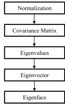
Figure 1. Eigenface process

Figure 1 describes the eigenface value search stage. First of all, the normalization process needs to be done to convert the image to a color intensity value. The set of colors is formed into a covariance matrix to be calculated. Once the eigenvalue and eigenvector are obtained, the eigenface can be generated.

III.

METHODOLOGY

Before the image is processed, the image is pre-processed. This process is done by converting RGB image to grayscale image to get a feature vector and get feature value to be used in the recognition process. The grayscaling stage of an image is an activity to simplify the image model. RGB is converted to one grayscale layer. The following equation is to change the RGB color into grayscale.

Before the image Matrix plays an important role to obtain an eigenface value. A two-dimensional matrix is formed to transform the pixel value of the image. The image consists of three components of the image will be converted into Grayscale. Here is the Eigenface process:

Normalization

Eigenvalues

Covariance Matrix

Eigenvector

- Create an EigenVectors list. This is a collection of N training images, where each image is W x H pixel. M is the number of eigenvectors to be created. - Combine each image in the WH vector element by

combining all the rows. Create an ImageMatrix as an N x WH matrix containing all the merged images - Add all rows to ImageMatrix and divide by N to get

a composite image. This is WH element vector with ψ.

- Reduce ImageMatrix with average image ψ. We call the new matrix the size of N x WH as Ф.

- Calculate the possible pairs of images. We get L as the Nx N size matrix where L [i] [i] = dot product of Ф [i] and Ф [j].

- Calculate the N eigenvalue and the corresponding vector. Take the eigenvector of M which has the highest eigenvalue. Each eigenvector has N element - Perform the matrix multiplication of each selected

vector M with Ф and store the result of a 1 x WH matrix.

IV.

RESULTS AND DISCUSSION

Evaluation

As the test material. There are three samples, A, B, C. Table 1 to 3 are three grayscale color matrix samples. Each table has different feature values.

Table 1. Sample A

3 21 93 117 98 167 185 168 222 138

99 177 188 233 150 101 71 30 87 61

81 100 92 230 149

Table 2. Sample B

105 157 65 161 69 98 224 29 160 177 156 203 229 191 153 177 31 53 8 33

74 111 65 209 138

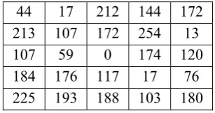
Table 3. Sample C

44 17 212 144 172 213 107 172 254 13 107 59 0 174 120 184 176 117 17 76 225 193 188 103 180

The eigenvector is obtained by adding the entire contents of the matrix with the same rows and columns. The result of the addition must be divided by the number of samples provided. In this test, there are three pieces of data into a sample. Table 4 is the result of an eigenvector.

EV(1,1) =

=

=

Table 4. Eigenvector

50.67 65 123.3 140.7 113 159.3 172 123 212 109.3 120.7 146.3 139 199.3 141

154 92.67 66.67 37.33 56.67 126.7 134.7 115 180.7 155.7

λa = ( ) ( )

=

=

Table 5. Eigenvalue of Sample A

-47.67 -44.00 -30.33 -23.67 -15.00 7.67 13.00 45.00 10.00 28.67 -21.67 30.67 49.00 33.67 9.00 -53.00 -21.67 -36.67 49.67 4.33 -45.67 -34.67 -23.00 49.33 -6.67

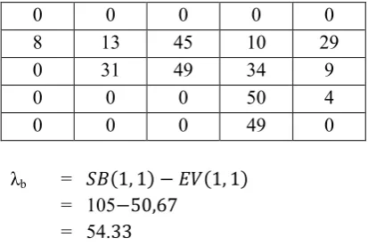
Table 6. Normalized Eigenvalue of Sample A

0 0 0 0 0

8 13 45 10 29

0 31 49 34 9

0 0 0 50 4

0 0 0 49 0

λb = ( ) ( )

= 105 = 54.

Table 7. Eigenvalue of Sample B

54,33 92,00 -58,33 20,33 -44,00 -61,33 52,00 -94,00 -52,00 67,67 35,33 56,67 90,00 -8,33 12,00 23,00 -61,67 -13,67 -29,33 -23,67 -52,67 -23,67 -50,00 28,33 -17,67

Table 8. Normalized Eigenvalue of Sample B

54 92 0 20 0

0 52 0 0 68

35 57 90 0 12

23 0 0 0 0

0 0 0 28 0

λc = ( ) ( )

= 44

=

Table 8. Eigenvalue of Sample C

-6.67 -48.00 88.67 3.33 59.00 53.67 -65.00 49.00 42.00 -96.33

-13.67 -87.33

-139.00 -25.33 -21.00 30.00 83.33 50.33 -20.33 19.33 98.33 58.33 73.00 -77.67 24.33

Table 9. Normalized Eigenvalue of Sample C

0 0 89 3 59

54 0 49 42 0

0 0 0 0 0

30 83 50 0 19

98 58 73 0 24

Tables 5 to 9 show the results of matrix normalization to obtain eigenvalue. The value below zero will automatically be zero so the calculation to find eigenvalue is easier. The creation phase of the eigenvalue in each sample has been completed. At the time of the test, it is required to have a matrix equal to that sample. Table 10 is an example of test data to be processed.

Table 10. Test

119 73 148 150 110 120 207 199 137 85 122 255 30 66 150 177 57 175 242 204 142 76 129 22 83

λt = T( ) ( )

= 119 = 68.33

Table 11. Eigenvalue of Test

68.33 8.00 24.67 9.33 -3.00 -39.33 35.00 76.00 -75.00 -24.33

1.33 108.67 -109.00 -133.33 9.00 23.00 -35.67 108.33 204.67 147.33 15.33 -58.67 14.00 -158.67 -72.67

Table 12. Normalized Eigenvalue of Test

68 8 25 9 0

0 35 76 0 0

1 109 0 0 9

23 0 108 205 147

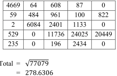
Tables 11 to 12 show the results of matrix normalization to obtain eigenvalue of test data. Each matrix has got eigenvalue. Similarities can be calculated based on the shortest distance using the Euclidean distance. Each sample will be tested to the test matrix. The lowest feature value is the most similar sample at the time of completion.

.

√∑( )

Table 13. Distance matrix of Test to Sample A

4669 64 608 87 0

59 484 961 100 822 2 6084 2401 1133 0 529 0 11736 24025 20449

235 0 196 2434 0

Total = √

=

Table 14. Distance matrix of Test to Sample B

196 7056 608 121 0

0 289 5776 0 4579

1156 2704 8100 0 9 0 0 11736 41888 21707

235 0 196 803 0

Total = √

=

Table 14. Distance matrix of Test to Sample B

4669 64 4096 36 3481 2880 1225 729 1764 0

2 11808 0 0 81

49 6944 3364 41888 16384 6889 3403 3481 0 592

Total = √ = 337.3878

From the above three results, the test matrix is closer to sample A. The result is similar to sample A.

V.

Eigenface is a good calculation in doing image matching. It can be done to test whether the image has been modified from the original or not. This technique can also examine an image whether inside the image contained confidential information by comparing the two images. The downside of eigenface is that light is very influential when comparing images. If there is the same object taken with two different lighting, then this will result in the object is very much different.

VI.

REFERENCES

[1].S. Maity, M. Abdel-Mottaleb and S. S. Asfour, "Multimodal Biometrics Recognition From Facial Video via Deep Learning," Signal & Image Processing : An International Journal, vol. 8, no. 1, pp. 1-9, 2017.

[2].P. K. Ghislain, G. L. Loum and O. Nouho, "Adaptation of Telegraph Diffusion Equation for Noise Reduction on Images," International Journal of Image and Graphics Vol. 17, No. 02, 1750010 (), vol. 17, no. 2, 2017.

[3].Arief, "Algoritma Eigenface," Informatika: Artikel Teknik Informatika dan Sistem Informasi, 8 January 2013. [Online]. Available: http://informatika.web.id/ algoritma-eigenface.htm. [Accessed 21 August 2017].

[4].M. A.-A. Bhuiyan, "Towards Face Recognition Using Eigenface," International Journal of Advanced Computer Science and Applications, vol. 5, no. 7, pp. 25-31, 2016.

[5].M. A. Imran, M. S. U. Miah, H. Rahman, A. Bhowmik and D. Karmaker, "Face Recognition using Eigenfaces," International Journal of Computer Applications, vol. 118, no. 5, pp. 12-16, 2015.

[6].A. P. U. Siahaan, "RC4 Technique in Visual Cryptography RGB Image Encryption," SSRG International Journal of Computer Science and Engineering, vol. 3, no. 7, pp. 1-6, 2016.