Compressive Sensing based Image Compression and Recovery

(1)

Compressive Sensing based Image Compression

and Recovery

Dr. Renuka Devi SM Associate Professor

Department of Electronics & Communication Engineering GNITS, Affiliated to JNTUH Hyderabad

Abstract

Compressive sensing is a new paradigm in image acquisition and compression. The CS theory promises recovery of images even if the sampling rate is far below the nyquist rate. This enables better acquisition and easy compression of images, which is more advantageous when the resources at the sender side are scarce. This paper shows the CS based compression and two recovery two methods i.e., l1 optimization and TSW CS recovery. Experimental results show that CS provides better compression, and TSWCS provides better recovery with less relative error recovery than l1 optimization. It is also observed that use of increased measurements leads to reduced error.

Keywords: Compressive Sensing, L1 Optimization, Tree Structured Wavelet (TSW)

________________________________________________________________________________________________________

I. INTRODUCTION

Image compression is playing an important role in the context of large volume of digital multimedia used over Internet. The objective of image compression is to reduce irrelevance and redundancy of the image data in order to be able to store or transmit data in an efficient form. Image compression can be lossy or lossless. Lossless compression is preferred for archival purposes and often for medical imaging and technical drawings.

The Shannon/Nyquist sampling theorem tells that in order to not lose information when uniformly sampling a signal must be sampled at least two times faster than its bandwidth. In many applications, including digital image and video cameras, the Nyquist rate can be so high that too many samples are to be taken and must compress in order to store or transmit them. In other applications, including imaging systems (medical scanners, radars) and high-speed analog-to-digital converters, increasing the sampling rate or density beyond the current state-of-the-art is very expensive. In [1,2,13,14] exhaustive literature survey on CS is done

Donoho[1] introduced the concept of compressed sensing where measurements are taken on transformed coefficients instead of samples. In compressive sensing[2,3], sampling and reconstruction operations with a more general linear measurement scheme coupled with an optimization in order to acquire certain kinds of signals at a rate significantly below Nyquist.

II. COMPRESSIVE SENSING THEORY[2]

Let X be a real valued, finite length, long one dimensional discrete time signal x, with elements x[n],n=1,2,3...N.A signal in RN can be represented in terms of a basis of N×1 vectors {ψi}i=1N . For simplicity assume that the basis is orthonormal. Forming N×N basis matrix Ψ ∶= [ψ1|ψ2| … … . ψN] by stacking the vectors as columns.

Then x can be represented as shown in equation (1)

X = ∑ siψi or X = ΨS (1) N

i=1

Where s represent N×1 weighing coefficients , si= < X, ψi> = ψiTX where .T denotes the transpose operation. Therefore X,S represent the same signal, X in time domain, S in Ψ domain.

If X is considered to be sparse in Ψ domain, i.e X can be represented by linear combination of just K basis vectors such that N-K other coefficients are zeros, and N-K<<N. Sparsity is motivated by the fact that many natural and manmade signals are compressible in the sense that there exists a basis where the representation (1) has just a few large coefficients and many small coefficients. Compressible signals are well approximated by K-sparse representations; this is the basis of transform coding.

(2)

(IJSTE/ Volume 3 / Issue 05 / 006)

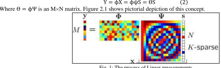
Consider the more general linear measurement process that computes M < N inner products between x and collection of vectors {ϕj}j=1M as in yj= < X, ϕj> Stacking the measurements into a M×1 vector Y and the measurement vectors ϕjT as rows into M×N matrix, so that Y is given by equation 2

Y = ϕX = ϕψS = ѲS (2) Where Ѳ = ϕΨ is an M×N matrix. Figure 2.1 shows pictorial depiction of this concept.

Fig. 1: The process of Linear measurements

The important point to note is the measurement process is non-adaptive; that is, ф does not depend in any way on the signal x. To achieve such a system of measurements

1) A stable measurement matrix has to be designed. 2) A recovery algorithm has to be designed.

– Stable Measurement Matrix

The design of stable measurement matrix is key to the compressive sensing system. From the M linear measurements that are measured, original N length vector X or S has to be reconstructed. If X does not exhibit sparsity it will be a ill-posed problem. As there are only K nonzero coefficients in S such that solving a system of M equations for K coefficients is sufficient for reconstructing S and eventually X.

A necessary and sufficient condition to ensure that this M × K system is well-conditioned and hence sports a stable inverse is that for any vector v sharing the same K nonzero entries as s, is given by equation (3.3)

1 − ϵ ≤‖ѲV‖2

‖V‖₂ ≤ 1 + ϵ , for ϵ > 0 (3)

In practice the K non-zero locations of S is unknown. But the sufficient condition for a stable inverse for both K sparse and compressible signals for Ѳ to satisfy (3.3) for an arbitrary 3K sparse vector V. This is called Restricted Isometric Property (RIP).

An alternative approach to stability is to ensure that the measurement matrix ф is incoherent with the sparsifying basis in the sense that the vectors {фj} cannot sparsely represent the vectors {ψi} and vice versa [2].

To accomplish the above conditions and verify RIP, a random matrix is taken as ф. If the elements of ф are taken as independent and identically distributed(iid) random variables, with zero mean and 1/N - variance Gaussian density. Then, the measurements y are merely M different randomly weighted linear combinations of the elements of x. A Gaussian ф has two interesting and useful properties. First, ф is incoherent with the basis, Ψ=I of delta spikes with high probability, since it takes fully N spikes to represent each row of ф. More rigorously, using concentration of measure arguments, an M × N i.i.d Gaussian matrix Ѳ = фI = ф can be shown to have the RIP with high probability if M > c K log(N/K), with c a small constant. In [13,14] exhaustive literature survey on CS is done.

III. DIFFERENT CS RECOVERY ALGORITHMS

CS[1] theory says that from M measurements the signal can be recovered exactly if condition in 3.4 is satisfied. M ≥ Const. K. logN (4)

Where Const is a over measuring factor greater than 1. Once the signal is represented by linear measurements in some orthonormal basis as y, in order to get back the signal X a number of reconstruction algorithms are used. As mentioned in [3,4,5] there are different reconstructions algorithms existing in literature. There are at least five major classes of computational techniques for solving sparse approximation problems.

Basis Pursuit[6]

The reconstruction algorithm is defined by a convex optimization problem. Solve the convex program with algorithms that exploit the problem structure. Most popular of this is l1 minimization.

(3)

Bayesian Framework[11]

Assume a prior distribution for the unknown coefficients that favors sparsity. Develop a maximum a posteriori estimator that incorporates the observation. Identify a region of significant posterior mass or average over most-probable models.

Non-Convex Optimization

Relax the ‘0 problem to a related non-convex problem and attempt to identify a stationary point.

Brute force

Search through all possible support sets, possibly using cutting-plane methods to reduce the number of possibilities.

Different algorithms and their combinations are used in the methods that are to be discussed. To apply any algorithm the basic condition to be satisfied for faithful reproduction of the signal is RIP (Restricted Isometric Property). The recovery technique used in reconstruction of image by CS measurements is the implementation is the basic pursuit with l1 minimization.

IV. IMPLEMENTATION DETAILS OF BASIS PURSUIT

The generalized implementation for optimization problems is l2 minimization. But in compressive sensing l1 minimization succeeds over l2 minimization. The problem of l1 minimization can be stated as in equation 3.5

Ŝ = argmin ‖S′‖₁such that ѲS′_{= Y (5)}

Geometrical Interpretation

To understand how l1 optimization is more suited for compressive sensing a geometric interpretation helps.

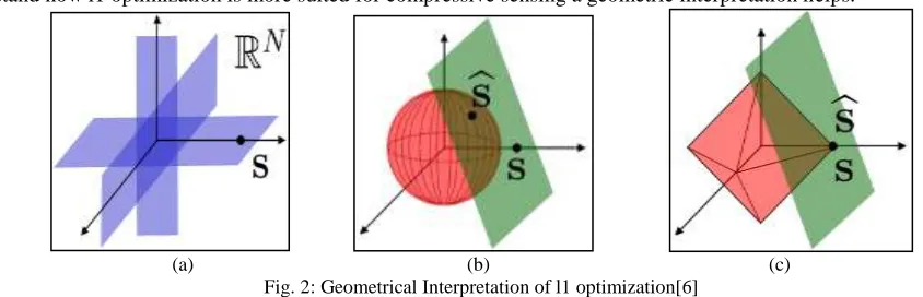
(a) (b) (c) Fig. 2: Geometrical Interpretation of l1 optimization[6]

Fig 2(a) shows a sparse vectors lies on a K dimentional hyperplane aligned with coordinate axes in RN and thus close to the axes. 2(b) shows that compressive sensing via l2 minimization does not find the correct sparse solution S on the translated null space. But 2(c) shows that through l1 minimization the correct sparse solution S can be recovered.

In other word if l2 minimization is considered, there will be many parellel hyperplanes that may be possible with minimum l2 distance. But when l1 minimization is considered there will be a unique hyperplane that closely approximate sparse plane S.

V. TREE STRUCTURE WAVELET CS (TSW CS)

He et al [10] has proposed a compressed sensing scheme based on Bayesian framework. The model is referred to as Tree Structured Wavelet Scheme (TSW)[10] where the properties of hierarchical wavelet model is fully exploited. This section discusses in detail about the TSW Scheme.

The Compressive Sensing concept takes N measurements of a data of M samples of data θ where N<<M. The N measurements are taken directly by random projections on to θ such that v = фθ. In the inverse problem θ must be inferred from v which is an ill-posed problem. The inverse problem is solved by l1 regularization.

(4)

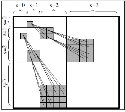
Fig. 3: Wavelet Decomposition of image

If θ is sparse, with S non-zero coefficients (S << M) then θ can be recovered from N measurements such that if N >

O(S. log (M/S)). Similar relationship holds good when θ is compressible but not exactly sparse.

The afore mentioned l1 regularization can be viewed as a maximum a posteriori estimate for θ under the assumption that each component of µ is drawn i.i.d. from a Laplace prior [11]. Based on this Bayesian compressive sensing algorithms are developed. These formulations are not fully utilizing the prior information on transform coefficients in θ. For example figure 3 shows the structure of wavelet coefficients when multiscale DWT is applied on a image.

The fig 2 shows the tree structured wavelet coefficients of a multi scale DWT of an image. The coefficients of top left block at S=0 corresponds to scaling coefficients that capture coarsest detail of the image. For 1< S < L-1 has four children coefficients corresponding to level S+1. The root coefficients act as Parent coefficients. These parent children relationship is modeled as a Hidden Marcov Tree (HMT) which is used in inversion of CS problem.

Compressive Sensing With Wavelet Transform Coefficients[10]

Let x be an M dimensional signal or image, which is sparse on wavelet basis vector, an M×M basis. The CS measurement v =

фψT_{x = фθ}_{, where}_ф_{is a N×M (N<<M) dimensional matrix of random projections.}_θ_{denotes M dimensional vector of wavelet}

transform coefficients. Suppose m coefficients of θ are significant and other M-m coefficients are negligible. Then θ = θm+ θe where θm represents the original θ with M-m smallest coefficients set to zero. θe represents the m significant coefficients set to zero. If the m significant coefficients are found out, the signal x can be closely approximated. So θe component is considered as noise ne. Further a noise component n0 is considered such that

v = фθm+ n

Where elements of n can be represented by a zero-mean Gaussian noise with unknown variance σ2_{, or unknown precision}_α

n=

σ−2

TSW Modeling

Tree-structured wavelet compressive sensing (TSW-CS) model is constructed in a hierarchical Bayesian learning framework. In this setting a full posterior density function on the wavelet coefficients is inferred. Within the Bayesian framework, a spike - and - slab model is imposed for Bayesian regression. The prior for the ith_{element of θ (corresponding to ith transform coefficient) has} the form shown in equation 4.2.

θi ~ (1 − πi) δ0 + πi 𝒩(0, αi−1), i = 1,2, … … . M, (7)

Which has 2 components. The first component δ0 is a point mass concentrated at zero, and the second component is a zero-mean Gaussian distribution with (relatively small) precision αi−1. the former represents the zero coefficients in θ and the latter the non-zero coefficients. This is a two-component mixture model, and the two components are associated with the two states in the HMT.

The mixing weight πi, the precision parameter αi, as well as the unknown noise precision αn, are learned from the data. The proposed Bayesian tree-structured wavelet (TSW) CS model is summarized as follows.

v θ

⁄ , αn ~ 𝒩(фθ, αn−1I ), (8)

(5)

πr ~ Beta(e0r, f0

r_{), (9c)}

πs0 ~ Beta(e0s0, f0s0), s = 2, … … L (9d) πs1 ~ Beta(e0s1, f0s1), s = 2, … … L (9e)

Where θs,i denotes the ith wavelet coefficient (corresponding to the spatial location) at scale s, for i= 1,2..., MS (MS is the total number of wavelet coefficients at scale s) , πs,i is the associated mixing weight, and θpa(s,i)denotes the parent coefficient of θ(s,i). In (9b) it is assumed that all the nonzero coefficients at scale s share a common precision parameter αs. It is also assumed that all the coefficients at scale s with a zero-valued parent share a common mixing weight πs0, and the coefficients at scale s with a nonzero parent share a mixing weight πs1.

VI. RESULTS

Experimental results are demonstrated over the cameraman image of 128x128 size significant part. The size of the image considered small, keeping in view of memory and computational requirements. Among the different choices available for l1 optimization schemes, l1 minimization with equality constraints is considered.

i.e.

min‖x‖₁ subjected to Ax = b (10)

For linear programming of l1 minimization problem Primal-dual barrier algorithm is used. Following are the results got using spgl solver for l1 optimization[9].

The simulation is iteratively done for 3000 samples to 6000 samples. The recovered image by TSW CS is seen to show fast convergence and great improvement quality by increasing number of CS measurements.

Table - 1

CS Recovery through l1 optimization and TSW CS method

No of Measurements Original Image Recovered Image (l1 Optimization) Recovered Image (TSW CS)

3000

Relative error=0.2181

4000

5000

(6)

6000

A graph representing number of CS measurements to relative reconstruction error is shown in the figure 4.2.

Fig. 4: Plot of CS Measurements Vs Relative Reconstruction error

VII.CONCLUSION

Compressive sensing on an image on DWT basis is implemented. TSW-CS method is found to be efficient in reconstruction of sparse coefficients when compared to CS recovery by l1 optimization. With fewer number of measurements better reconstruction quality can be achieved by using Bayesian regression along with employing wavelet statistical properties. The above results show that as number of CS measurements are increased, the recovered image quality increases. After certain limit if we increase number of CS measurements, the recovery takes very long time, as the complexity of l1- optimizer is O(N3_{) operations.}

REFERENCES

[1] Donoho D.L., “Compressed sensing,” IEEE Transactions on Information Theory, vol. 52, pp. 1289–1306, 2006.

[2] Cand`es E. J. and Wakin M. B., “An introduction to compressive sampling,” IEEE Signal Processing Magazine, vol. 25, pp. 21–30, 2008.

[3] Tropp, Joel A., and Stephen J. Wright. "Computational methods for sparse solution of linear inverse problems." Proceedings of the IEEE 98.6 (2010): 948-958.

[4] Candès E., Romberg J. and Tao T., “Robust uncertainty principles: Exact signal reconstruction from highly incomplete frequency information,” IEEE Trans. Inform. Theory, vol. 52, no. 2, pp. 489–509, Feb. 2006.

[5] Tropp, Joel A., and Stephen J. Wright. "Computational methods for sparse solution of linear inverse problems." Proceedings of the IEEE 98.6 (2010): 948-958.

[6] J. A. Tropp and A. C. Gilbert, “Signal recovery from random measurements via orthogonal matching pursuit,” IEEE Transactions on Information Theory, vol. 53, pp. 4655–4666, 2007.

[7] D. L. Donoho, Y. Tsaig, I. Drori, and J.-L. Starck, “Sparse solution of underdetermined linear equations by stagewise orthogonal matching pursuit,” March 2006, preprint.

[8] B. Efron, T. Hastie, I. Johnstone, and R. Tibshirani, “Least angle regression,” Annals of Statistics (with discussion), vol. 32, pp. 407–499, 2004. [9] [Online]. Available: http://www.cs.ubc.ca/~mpf/spgl1/

[10] Deng C.W., Lin W. S., Lee B. S. and Lau C. T., “Robust image compression based upon compressive sensing,” in Proc. IEEE Int. Conf. Multimedia and Expo. (ICME’10), Jul. 2010, pp. 462–467.

[11] Ji S., Xue Y., and Carin L., “Bayesian compressive sensing,” IEEE Transactions on Signal Processing, vol. 56, 2008, pp. 2346–2356.

[12] Said A. and Pearlman W. A., “A new, fast, and efficient image codec based on set partitioning in hierarchical trees,” IEEE Transactions on Circuits and Systems for Video Technology, vol. 6, 1996, pp. 243–250.