Calculation the eigenvalues of the power-law and logarithmic potentials using the J-matrix method

(1)

Calculation the eigenvalues of the power-law and

logarithmic potentials using the J-matrix method

Afaf Abdel-Hady

Faculty of Engineering, Al-Asher University, Al-Asher City, Egypt E-mail: [email protected]

Abstract

--

The eigenvalues of the power-law and

logarithmic potentials are calculated using the J-matrix method. The calculations are carried out for states with arbitrary

quantum numbers n and . Comparisons are made with the available literature data and excellent agreement is observed. In all the cases, the current method yields considerably improved results over the other existing calculations. Some new states are reported for guiding future comparisons.

Index Term

--

J-matrix method, Complex rotation, eigenvalues, power-law potential, logarithmic potential.

Pacs number: 03.65.Ge, 31.15.Bs, 02.30.Mv

I. INTRODUCTION

Since the appearance of the J-matrix method [1], it has been proven to be a suitable method to calculate the bound and resonance state energies, as well as the phase shift and scattering matrix for different potentials in the field atomic, molecular and nuclear systems. So far, the potentials that have been done are: the Morse and inverse Morse [2] potentials,

exponential-cosine-screened Coulomb potential [3], Yukawa [4] and tamed Yukawa potentials [5], and the Hellmann potential [6].

To test the J-matrix method for potentials, we are devoting this work to determine the bound state spectra of the power-law and the logarithmic potentials accurately. As mentioned earlier [7], the given potentials have relevant applications in the field of particle physics [8,9]. These potentials have been studied from various perspectives by several researchers employing a number of approximations, e.g., the WKB treatment [10], the shifted 1/N expansion method [11,12], the variational technique [13], generalized pseudo-spectral (GPS) method [7], through an interpolation formula [14], and also by the direct numerical integration methods [10,14]. Although several formally attractive and elegant formalisms exist in the literature, there is a lack of accurate eigenvalues, especially for those states characterized by higher quantum numbers. As is demonstrated in section 3, it appears that the current method produces excellent results in the systems under study, for both low high states.

The layout of the paper is as follows: Section II presents a brief overview of the method of calculation. In section III we present the results for the power-law and the

logarithmic potentials. Finally, in section IV we conclude with few remarks.

II. THEORETICAL FORMULATION

The details of our theoretical calculations are already presented in earlier work [2], so we will only present the essentials. In the following equations, we have used the atomic units = m = e = 1 and length is measured in the units

of

a

₀



4 

ò

₀ 2

me

2. The symbol is for the angular momentum quantum numbers, Z for the atomic charge, and E for the total energy. The main idea of the J-matrix method is based on expanding the wave function



( )

r

in the one-particle Schrödinger wave equation (in atomic units):





22 2

1 (

1)

( )

0

2

2 d

Z

H

E

r

V r

E

r

dr

r













 

_





_







, (2.1)

into a complete Laguerre basis set



 

_n

(

r

)



in the form:

1 2 2 1

( )

x

( )

n

x

a x

n

e

L

n

x



_

  

;

0,1, 2,..

n



(2.2)

where

x





r

,





0

, and  is a positive length scale parameter.

L

2_n 1

( )

x

is the Laguerre polynomial, and

a

_n is the normalization constant



 

(

n

1)

 

(

n

2 

2)

. The basis (2.2) is chosen to form the matrix representation of the

reference Hamiltonian:

H

_o (



H



V

) tridiagonal. The

basis set



 

_n

(

r

)



is chosen to satisfy the boundary condition

(

)

0

n

r

 



at

r



0

and as

r

 

. The reference Hamiltonian

H

₀ in this representation is therefore fully accounted for, whereas the potential V is approximated by its representation in a subset of the basis, such that

 

;

,

1

o _nm nm nm

o nm

H

V

n m

N

H

n m

N











 

_

_



.

(2)

The calculation of the matrix elements of the effective potential V(r) is usually obtained by evaluating the integral:

0

(

) ( )

(

)

nm n m

V







 

r V r

 

r dr

(2.4)

The evaluation of such an integral, for a general effective potential, is always done numerically or by using the Gaussian quadrature approximation [15]. The above representation (2.3) is the fundamental underlying feature of the J-matrix method, taking into account that the full reference Hamiltonian should result in a substantial improvement on the accuracy of the results. This is the whole purpose of the J-matrix approach that they are proposing [1].

In the following section, we will implement the above approach numerically to find the bound states of the

potentials

V r

( )



r

0.5 and

V r

( )



ln

r

. This will illustrate the accuracy of this method and determine the advantage of this procedure compared to other approaches.

III. RESULTS AND DISCUSSIONS

Following our previous work [2-6], we will follow the given steps:

1- Perform the



–plateau to study the stability of the bound state energies for different



. This is done first by using fixed values of

N

, for example

70 N



, and for different values of



, where we check the variation of fixed energy with changing



. Doing this, the values of



we found are as given in tables (1) and (2).

2- For fixed N and



, we start to calculate the ground states energies.

3- By changing N, or



, by one, we can only keep the matching digits between the two values.

So, the results are reported only up to the precision that maintained stability, and all our results are truncated rather than rounded-off. Thus, all the results may be considered as correct up to the place they are reported.

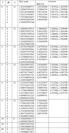
Table 1 shows the results of the current method for the

excited states of different values of and n for the r0.5 potential using

N



150

. For all values of



5

and

5 n



, our results and GPS results are in excellent agreement up to the 8th digit given in [7]. The variational results [12] are consistently overestimated in all cases except the third and fourth states belonging to



0

. Table 1 contains new

results,



10

and

n



0,1

, that are unique to our approach since the values of the potential parameters and range of energies fall outside the applicability of most perturbative and variational calculations found elsewhere.

Table 2 displays the computed eigenvalues for selected n

and quantum numbers of the logarithmic potential using

150 N



. For all values of



4

, and

n



5

,

5  

10

,

and

n



0,1

our results and GPS results are in excellent agreement up to the 8th digit given in [7]. Table 2 contains new results, with



10

and

n



0,1

, that are unique to our approach, since the values of the potential parameters and range of energies fall outside the applicability of most perturbative and variational calculations found elsewhere.

IV. CONCLUSION

In summary, we have computed bound state energies associated with the power and logarithmic potentials using the J-matrix technique. Both potentials were generated and compared favorably with those in the literature [7,10, 12-14] for different values of the quantum numbers n and . Finally we would like to stress that this approach could easily be

generalized to handle other short-range potentials with

r



singularity (analytic and non-analytic) as well as multi-channel scattering potentials.

ACKNOWLEDGMENT

The author thanks Professor I. Nasser for encouragement and discussions. The work was supported by Al-Asher University.

REFERENCES

[1] Heller E. J. and Yamani H. A., Phys. Rev. A 9, 1201 (1974); ibid.

1209 (1974); Alhaidari A. D., Heller E. J., H. A., and Abdelmonem M. S. (Eds.), The J-matrix method: Recent Developments and Selected Applications (Springer, Heidelberg, 2008).

[2] Nasser I., Abdelmonem M. S., Bahlouli H. and Alhaidari A. D., J. Phys. B: At. Mol. Opt. Phys. 40 4245 (2007); ibid. 41, 215001 (2008).

[3] I. Nasser, M. S. Abdelmonem and Afaf Abdel-Hady, Phys. Scr. 84, 045001 (2011).

[4] Bahlouli H, Abdelmonem M S and Nasser I Phys. Scr.82 065005 (2010)

[5] Abdelmonem M. S., Nasser I., Bahlouli H., Al Khawaja U., and Alhaidari A. D., Phys.Lett. A 373, 2408 (2009).

[6] I. Nasser,and M. S. Abdelmonem, Phys. Scr. 83, 055004 (2011). [7] Roy A K J. Phys. G: Nucl. Part. Phys. 30 269 (2004). [8] Quigg C and Rosner J L Phys. Lett. B 71 153 (1977).

[9] Martin A Phys. Lett. B 93 338 (1980); Magyari E Phys. Lett. B 95

295 (1980); Barik N and Jena S N Phys. Lett. B 97 265 (1980); Martin A Phys. Lett. B 100 511 (1981); Jena S N and Rath D P Phys. Rev. D 34 196 (1986); Barik N, Jena S N and Rath D P Phys. Rev. D 41 1568 (1990); Akcay H and Ciftci H J. Phys. G: Nucl. Part. Phys. 22 455 (1996); Jena S N, Panda P and Tripathy T C Phys. Rev. D 63 014011 (2000); Jena S N, Panda P and Tripathy T C J. Phys. G: Nucl. Part. Phys. 27 227 (2001).

(3)

[11] Sukhatme U and Imbo T Phys. Rev. D 28 418 (1983); Maluendes S A, Fern´andez F M, Mes´on A M and Castro E A Phys. Rev. D 34

1835 (1986).

[12] Imbo T, Pagnamenta A and Sukhatme U Phys. Rev. D 29 1669 (1984).

[13] Ciftci H, Ateser E and Koru H J. Phys. A: Math. Gen. 36 3821 (2003).

[14] Hall R L J. Phys. G: Nucl. Part. Phys. 26 981 (2000).

[15] See, for example, Appendix A in: A. D. Alhaidari, H. A. Yamani, and M. S. Abdelmonem, Phys. Rev. A 63, 062708 (2001).

Table I

The eigenvalues E (in au) of the

r

0.5potential along with the literature data for different values of and

n

at

N



150

.

n



This work Literature

Ref [7]

0 0 1 2 3 4 5 6

12 1.833393609777 2.550647491414 3.051181948950 3.452131943857 3.793360444647 4.093925845294 4.364629591366 1.83339360 2.55064749 3.05118194 3.45213194 3.79336044 4.09392584 1.83352a, 1.83339b 2.55152a, 2.55065b 3.05177a, 3.05118b 3.45197a, 3.45213b 3.79233a, 3.79336b

1 0 1 2 3 4 5 6

12 2.300496239515 2.854335925747 3.285833295818 3.647385421454 3.962676500693 4.244658384223 4.501278847349 2.30049623 2.85433592 3.28583329 3.64738542 3.96267650 4.24465838 2.30056a, 2.30050b 2.85473a, 2.85434b 3.28666a, 3.28583b 3.64838a, 3.64739b 3.96361a, 3.96268b

2 0 1 2 3 4 5 6

12 2.657563368283 3.120328492061 3.502451547428 3.832543915845 4.125809074413 4.391385732370 4.635241055468 2.65756336 3.12032849 3.50245154 3.83254391 4.12580907 4.39138573 2.65760a, 2.65756b 3.12048a, 3.12033b 3.50296a, 3.50245b 3.83338a, 3.83254b 4.12686a, 4.12581b

3 0 1 2 3 4 5 6

12 2.954450931022 3.357591349991 3.702704997614 4.007367339627 4.281959441721 4.533168655526 4.765579659797 2.95445093 3.35759134 3.70270499 4.00736733 4.28195944 4.53316865 2.95448a, 2.95445b 3.35764a, 3.35759b 3.70299a, 3.70270b 4.00796a, 4.00737b 4.28282a, 4.28196b

4 0 1 2 3 4 5 6

12 3.212334372663 3.572752671355 3.888975640420 4.172681906044 4.431306273433 4.669897411225 4.892054212354 3.21233437 3.57275267 3.88897564 4.17268190 4.43130627 4.66989741 3.21236a, 3.21233b 3.57275a, 3.57275b 3.88913a, 3.88898b 4.17308a, 4.17268b 4.43196a, 4.43131b

5 0 1 2 3 4 5 6

12 3.442445619449 3.770419297358 4.063360362146 4.329479332953 4.574304302306 4.801747995367 5.014689710935 3.44244561 3.77041929 4.06336036 4.32947933 4.57430430 4.80174799

10 0 1

8 4.349403904773 4.585692768155 20 0

1

5.605352457522 5.769146840726 40 0

1

7.305735661325 7.416686577873

(4)

a Reference [12]. b Numerical results [14].

Table II

The eigenvalues E (in au) of the ln r potential along with the literature data for different values of and

n

at

N



150

.

n



This work Literature

Ref [7]

0 0

1 2 3 4 5 6 7

12 1.04433226735 1.84744258025 2.28961571416 2.59570686744 2.82992843684 3.01965502636 3.17910756863 3.31662376715 1.04433226 1.84744258 2.28961571 2.59570686 2.82992843 3.01965502 3.17910756 3.31662376

1.04436a, 1.0445b, 1.0443c 1.84457a, 1.8485b, 1.8474c 2.28417a, 2.2903b, 2.2897c 2.58863a, 2.5957b, 2.5957c 2.82176a, 2.8293b, 2.8299c

3.16956a, ,3.179 11c

1 0

1 2 3 4 5 6 7

8 1.64114133651 2.15094678797 2.49094221169 2.74559643790 2.94900787781 3.11827840918 3.26318814885 3.38984841774 1.64114133 2.15094678 2.49094221 2.74559643 2.94900787 3.11827840 3.26318814 3.38984841

2 0

1 2 3 4 5 6 7

6 2.01330864205 2.38743285046 2.66249204070 2.87949935701 3.05848949467 3.21070014612 3.34304953564 3.46009243781 2.01330864 2.38743285 2.66249204 2.87949935 3.05848949 3.21070014

3 0

1 2 3 4 5 6 7

6 2.28414135337 2.57978331293 2.81044538680 2.99916581946 3.15866751875 3.29668751384 3.41826920502 3.52687725904 2.28414135 2.57978331 2.81044538 2.99916581 3.15866751 3.29668751

4 0

1 2 3 4 5 6

6 2.49711469632 2.74154358798 2.94004751935 3.10686428381 3.25056363456 3.37668462581 3.48900541711 2.49711469 2.74154358 2.94004751 3.10686428 3.25056363 2.499c 2.742a 2.941c

3.10629a, 3.1071b, 3.107c 3.24960a, 3.2512b, 3.251c

5 0

1

6 2.67263174350 2.88099141157

2.67263174 2.88099141

6 0

1

6 2.82191040514 3.00348669662

2.82191040 3.00348669

7 0

1

6 2.95178152014 3.11268074478

2.95178152 3.11268074

8 0

1

6 3.06671400951 3.21116668545

3.06671400 3.21116668

9 0

1

6 3.16979180357 3.30084996746

(5)

10 0 1

6 3.26323280402 3.38317071523

3.26323280

20 0 1

4 3.90094090445 3.96583217398 30 0

1

4 4.28723372790 4.33171359706

50 0 1

4 4.78245721969 4.80976117093

a Reference [12]. b Reference [13].