A ZMP Feedback Control
for Biped Balance and its Application to
In-Place Lateral Stepping Motion
Satoshi Ito
∗,†, Shinya Amano
∗Minoru Sasaki
∗and Pasan Kulvanit
‡ ∗Faculty of Engineering, Gifu University, Gifu 501-1193, Japan
†
BMC Research Center, RIKEN, Nagoya 463-0003, Japan
‡
Institute of Field Robotics, King Mongkut’s University of Technology Thonburi, Bangkok, Thailand
Email:
{satoshi, sasaki}@gifu-u.ac.jp, [email protected]
Abstract— Many biped robot control schemes adopt a zero moment point (ZMP) criterion, where the motion is initially planned as the positional trajectories such that ZMP stays within the support polygon, while the feedback control of each joint is later applied to follow the planned reference motion. Although this method is powerful, the ZMP is not always controlled in a feedback manner. Namely, when the environment such as the gradient of the ground varies, the planned motion may cause the tumble and so replanning or modification is sometimes required in order to avoid it. With respect to the environmental variations, the ZMP trajectory is invariant in the lateral plane of the biped robot, in which the ZMP moves from the one side to the other and vice versa. From this point of view, we propose a biped control method for the frontal plane motion based on the ZMP position feedback . It does not required the reference motion of the upper body and the motion replanning or modification of the reference motion are free against environmental variation. This method is applied in the in-place stepping motion and the stability of this method is examined analytically as well as by computer simulations. Finally, the effectiveness of this method is demonstrated by the robot experiment with some improvement points.
Index Terms— biped robot, stepping motion, Center of pressure, motion planning, adaptive behavior
I. INTRODUCTION
The main problem of a biped control is maintaining balance. The tendency to fall can be determined based on the zero moment point (ZMP) [1] obtained as a cross point of the inertial and gravitational force resultant vector and the ground. Many studies of biped walking utilized the so-called ZMP criterion [2]–[5]: the reference trajectories of each joint angle, or the center of mass (CoM) of the body, are initially planned to force the computed ZMP based on the planned motion to stay inside the foot support. The joint angles, or the CoM of the body, are then controlled in a feedback manner to follow these reference trajectories. However, this strategy does not directly control the ZMP since the actual position of the ZMP is not measured This paper is based on “In-place lateral stepping motion of biped robot adapting to slope change” by S. Ito, S. Amano, M. Sasaki, and Pasan Kulvanit, which appeared in the Proceedings of IEEE International Conference on Systems, Man, and Cybernetics (SMC 2007), Montreal, Canada, October 2007. c°2007 IEEE.
during the locomotion. In other words, the ZMP position is ensured only by the accurate realization of the reference trajectories, implying that the modeling error such as irregularities of the ground surface may disturb the ZMP trajectory from the planned one. Although some studies introduced the concept of the ZMP feedback [6]–[9], or on-line trajectory planning based on ZMP position [10]–[13], however, the stability is not discussed except in a few papers [14], [15]. In addition, some of them require accurate model of the links system, which contains complex calculations as well as the utilization of dynamic parameters such as the moment of the inertia which are usually difficult to obtain.
The control of the lateral motion during biped walk is a good candidate for the ZMP feedback control, where the ZMP is selected as a control variable. A complete walking motion is composed of sagittal plane motion characterized as an inverted pendulum motion and lateral plane motion. The control principles are different between the two. The purpose of the sagittal plane motion is the spatial migration by transferring the support legs, indicating that the forward-falling motion of the inverted pendulum is essential. On the other hand, for the lateral plane motion, the body weight shifts to make one leg lifted up without falling. Focusing on this nature of balance keeping, our scope is restricted here to the motion control in the lateral direction throughout this paper. The weight shift is represented as the lateral movement of the CoP (center of pressure) that is equivalent to the point where total body weight is placed. Thus, it is natural to select the CoP as a control variable. Goswami [16] states that the ZMP is identical to the CoP. This implies that our method is equivalent to the ZMP feedback control.
Therefore, we aim here at controlling the position of the CoP to follow the reference trajectory. From the viewpoint of static balance, a method that utilizes feedback of the position of the CoP was proposed by [17] and [18]. Now this method is applied to a weight shift motion by making the reference position of CoP time-varying [19] and extended a motion control method for lateral in-place stepping [20]. Because the CoP and ZMP are identical [16], it is equivalent to the balance control based on the ZMP feedback. This method requires no reference trajectory of the body motion. Furthermore, this control law can be constructed without dynamical parameters of the biped link model. Such body’s trajectory-free and dynamical parameter-free feature gives the contribution to the biped control in the aspect of the robustness as well as the reduction of the computational cost.
Summing up the mathematical analyses and robot ex-periments in our previous works [19], [20], this paper is structured as follows. In section II, the fundamental theory of the CoP, i.e., ZMP feedback control, is described. This theory is extended first to the weight shift movement in double support phase in section III. Based on these two sections, a new control strategy for stepping motion is proposed, and computer simulation results are shown in section IV. In section V, the details of our experimental apparatus are introduced and experiment results of the in-place lateral stepping motion are presented. The con-cluding remarks are given in section VI.
II. BALANCE CONTROL BYCOPREGULATION Ground reaction forces include significant information necessary for balancing control. A model-free control law effectively utilizing them such that a static balance can be maintained by changing the posture adaptively with respect to the unknown constant external forces [18].
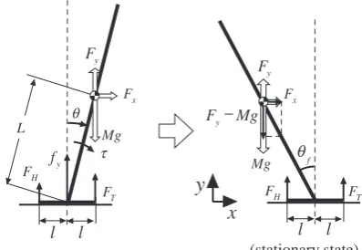
Assumptions of the control law are as follows. The body link and the foot link are connected at the ankle joint as illustrated in the left figure of Fig. 2. The motion occurs only in the sagittal plane. The ankle joint angle
θ and its velocity θ˙ are detectable, while appropriate torqueτ is actively generated at the ankle joint. The foot link has two ground contact points at the heel and the toe, where the vertical component of the ground reaction force FH and FT, are measurable. The foot does not slip on the ground and its shape is symmetrical in the anterior-posterior direction. The ankle joint is located at the midpoint of the foot link with zero height.
Suppose an unknown constant external force is exerted at the center of mass (as shown in Fig. 2), whose hori-zontal and vertical component isFx andFy, respectively. If balance is kept, only the body link has dynamics which is described in the following equation of motion.
Iθ¨ = M Lgsinθ+FxLcosθ−FyLsinθ+τ.
= ALsin(θ−θf) +τ (1) where
A=
q
(M g−Fy)2+Fx2 (2)
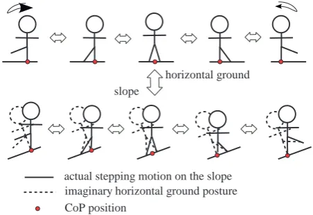
horizontal ground slope
imaginary horizontal ground posture actual stepping motion on the slope
CoP position
Fig. 1. Lateral stepping motion on different gradient condition.
andθf is a constant satisfying
sinθf =−
Fx
A, cosθf =
M g−Fy
A . (3)
And, M is a mass of the body link, I is its moment of inertia about the ankle joint,L is the length between the ankle joint and the center of mass (CoM) of the body link andg is the gravitational acceleration.
The goal of the control is to keep the postural balance regardless of the constant external force Fx and Fy. It is most effectively achieved by making FT and FH equal from the aspect of the stability margin. One of the solutions can be stated by the following theorem.
Theorem 1: For the dynamical system (1), consider the torque input τ as follows:
τ =−Kdθ˙+Kp(θd−θ) +Kf Z
(FH−FT)dt. (4) If feedback gain Kd,Kp andKf satisfy the conditions
Kp> AL >0 (5)
`
IKd > Kf >0 (6)
(Kd`−KfI)Kp> Kd`AL, (7)
then, FH =FT holds at the stationary state and θ=θf becomes a locally asymptotically stable posture.
Proof: First, we define a new state variable τf by the following equation,
τf = Z
(FH−FT)dt. (8) Substituting (4), (1) turns to
Iθ¨ = ALsin(θ−θf)
−Kdθ˙+Kp(θd−θ) +Kfτf, (9)
On the other hand, the ground reaction forces are de-scribed with ankle joint torque as,
FT =−1
2`τ+
1 2mg+
1
2fy, (10)
FH = 1
2`τ+
1 2mg+
1
L Mg
y
f θ
τ
x F y
F
T F H
F Mg
x F y
F
T F H
F f θ
Mg Fy−
(stationary state)
x
y
l l l l
Fig. 2. Link model for static balancing.
where m is a mass of the foot link and ` is the length from the ankle joint to the toe or the heel, and fy is the vertical component of the force from the body link.
Differentiating (8) and then substituting (10), (11) and (4), we obtain
˙
τf = 1
`(−Kdθ˙+Kp(θd−θ) +Kfτf). (12)
The dynamical system described by (9) and (12) have an equilibrium point(¯θ,τ¯f),
(¯θ,τ¯f) = (θf,
Kp
Kf(θf−θd))
(13) Note that FH = FT, because τ˙f = 0 at the stationary state. By analyzing the stability of this equilibrium point with the linearized equations, (5)-(7) can be derived from Routh/Hurwitz method.
The stationary posture is illustrated in the right figure of Fig. 2. The moment about the ankle joint, produced by the gravity and external forces, becomes zero, which achieve an effective maintenance of the stationary posture. The control law (4) is equivalent to the feedback control of CoP. The resultant moment of the vertical component of all the ground reaction forces become zero around the CoP. Using this property, the CoP position is calculated as follows,
PCoP = FT`−FH`
FT +FH ,
(14) where, PCoP is the horizontal position of CoP from the ankle joint. If the motion is slow, FT +FH represents total weight of the link system and thus can be regarded as constant. Defining constantKw as
Kw= `
FT +FH,
(15) the above equation changes to
PCoP =−Kw(FH−FT). (16)
Using this relation, (4) can be written as a form of the CoP position feedback
τ = −Kdθ˙+Kp(θd−θ)
+K0 f
Z
(Pd−PCoP)dt. (17)
length, angle and position
mass, force and torque
B
l
l
Bf
l
l
ff
l
l
fl
l
Fig. 3. A link model for double support phase .
This equation has been extended to include Pd, the reference position of the CoP (see also sec. IV), that was set to zero in (4), i.e., FH−FT →Fd ≡0 whereFd is the reference value. Here,K0
f=Kf/Kwis also constant. III. WEIGHT SHIFT MOVEMENT BY TIME-VARYING
COPREFERENCE IN DOUBLE SUPPORT PHASE The control law (4) allows the stationary posture to adaptively change with the environmental conditions, since θf is determined by Fx andFy. Here, this control law is extended for the biped double support phase. This extension mainly makes the reference of the CoP, which was constant in the static balance control, to be time-varying. Then, an adaptive bilateral motion is expected to emerge by the CoP control without generating body’s reference trajectories.
A. A link model for double support phase
zero height. At the end of both sides, the foot comes into contact with the ground, and the ground reaction forces are detectable. Furthermore, angular positions and angular velocities are measurable at the ankle and the hip joints. Every joints are actively actuated.
B. Control law
The degree of freedom (DoF) of the link model in the normal double support phase where the foot links keep contact with the ground, as shown in Fig. 3, is one, since the body link and two leg links construct a close mechanism. Because the control law (4) is also derived for stabilizing 1 DoF inverted pendulum motion, it could be extended to the bilateral balancing by addressing the following three points. First, there are two more contact points than the previous case. Second, the orbit of the CoG motion is not an exact circle. Third, the actuation is redundant. To solve these three problems, the control law is extended as follows.
1) Description of CoP: The added number of the contact points is an obvious difference. This problem is solved by introducing the concept of CoP. The control law (17) is available regardless of the number of the contact points. In the double support phase, the position of CoP, PCoP, is calculated from the vertical component of ground reaction forces at four contact points, i.e.,FRO,
FRI,FLO, andFLI.
PCoP = −FRO
Fall(xf+`f)−
FRI
Fall(xf−`f)
+FLI
Fall
(xf−`f) +FLO
Fall
(xf+`f) (18)
Fall = FRO+FRI +FLI +FLO. (19)
Here, the subscript RO, RI, LI and LO respectively represent the position of contact point, which are, the right outside, the right inside, the left inside, and the left outside. `f is the length from the ankle joint to the side of the foot link.xf is the distance to the ankle joint from the origin of the coordinates set at the midpoint of both ankle joints.
2) Coordinate frame for CoG motion: Although the CoG motion draws a circular arc in the biped upright model in Fig. 2, it generally does an elliptic arc in the double support model in Fig. 3 since the length between both feet is not the same as the one between both hip joints.
To solve this problem, the new coordinate frame is introduced. Here, the coordinate of CoG on this frame is presented byφ. It is preferable that this coordinate frame is naturally extended from the one for the single support phase. From this point of view, we define φas the sway angle of CoG from the vertical direction.
φ= arctanxG
yG.
(20) Here, (xG, yG) denotes the coordinate of CoG whose origin is set at the midpoint between both foot. Using
the ankle joint angle in both side, θRA and θLA, the coordination of CoG can be described as
xG= 2ρcosθRA+θLA
2 sin
θRA−θLA
2 (21)
yG = 2ρcosθRA+θLA
2 cos
θRA−θLA
2 (22)
Here,
ρ= 2m`+M L
2(2m+M). (23) Using this relation, we obtain
xG
yG
= tanθRA−θLA
2 (24)
According to the definition of the generalized coordinate (20),φis expressed as
φ= θRA−θLA
2 . (25)
The generalized force τφ is also defined as the torque exerted in the tangential direction of the orbit. Based on (4) and the relation PCoP =PZM P, here PZM P is the position of the ZMP, τφ is determined as follows:
τφ = −Kdφ˙+Kp(φd−φ)
+Kf Z
(Pd−PZM P)dt (26) Since this equation takes the same form as (4), the COP (ZMP) is expected to converge to the desired value.
3) Joint torque calculation: Next, we calculate the joint torque which produce the generalized force τφ. When CoG moves ∆φ along the orbit, the hip and ankle joints also changes, the amount of which is put to ∆θ (θ = [θRA, θRH, θLH, θLA]). The subscript RA, RH, LH and LA represent the joint position, which are, the right ankle, the right hip, the left hip, and the left ankle, respectively. The relation between ∆θ and∆φis described using the Jacobian matrix J(θ) as
∆θ=J(θ)∆φ. (27) In the coordinate frame defined in this section, the J(θ) is calculated as follows. From (25)
˙
φ= θ˙RA−θ˙LA
2 (28)
is satisfied. In addition, a kinematical relation among the joint angle are given as
−θRA+θRH+θLH−θLA=π (29)
Its differentiation becomes
−θ˙RA+ ˙θRH+ ˙θLH−θ˙LA= 0 (30)
Now, the coordinate of the left hip joint (xRH, yRH)can be described as two ways:
·
xRH
yRH ¸
=
·
−xf+LsinθRA
LcosθRA ¸
=
·
xf−LsinθLA−2`Bsin(θLH−θLA)
LcosθLA−2`Bcos(θLH−θLA) ¸
Differentiating them, the following two equations are obtained.
·
−Lθ˙LAcosθLA−2`B( ˙θLH−θ˙LA) cos(θLH−θLA)
−Lθ˙LAsinθLA+ 2`B( ˙θLH−θ˙LA) sin(θLH−θLA) ¸
=
·
Lθ˙RAcosθRA
−Lθ˙RAsinθRA
¸
(32) Solve the three equations (28), (30), (32) as four variables
˙
θ = [ ˙θRA,θ˙RH,θ˙LH,θ˙LA]T, and the relation betweenθ˙ andφ˙ is represented by
˙
θ= 2
J1+J3
J1
J1−J2
J2−J3
−J3
φ˙=J(θ) ˙φ (33)
J1= 2`BsinθLH (34)
J2=Lsin(θLH+θRH) (35)
J3= 2`BsinθRH. (36)
From the principle of virtual work, the next relation holds between the generalized force τφ and the joint torques τ= [τRA, τRH, τLH, τLA],
τφ=JT(θ)τ (37)
Solving this equation, the joint torques are given by
τ = (JT(θ))∗τ
φ+ (I−JT(θ)(JT(θ))∗)p (38) Here, ∗ denoted its generalized inverse matrix, and p is an arbitrary 4-dimensional vector.
C. Stationary state
Let us discuss the stationary state that is achieved by the control law (26). Here, assume that the joint angles can be described as a function of φ, i.e.,θ=θ(φ), which is possible if0< θRH, θLH< π. Note that the tangent line of CoG orbit is not orthogonal to the ground in the range of the normal lateral motion. The equation of motion can be described using φas
M(θ) ¨φ+C(θ,θ˙) +G(θ, g,F) =τφ. (39) where, Gcontains not only the gravity but also external force F, i.e., Fx and Fy in (1). From the mechanical property,M(θ)>0andC(θ,θ˙)become the second order term ofθ˙. On the other hand, the joint torque control the CoP through τφ, whose relation is expressed as
PCoP =P(θ)τφ+Q(θ,θ˙) +R(θ, g,F) (40) Now, we have defined the control inputτφby (26). For the simplicity of calculation of stationary state, a new state variableτf is introduced
τf = Z
(PZM P −Pd)dt= Z
(PCoP−Pd)dt (41) Then, the equation of motion (39) forφbecomes
M(θ)¨θ+C(θ,θ˙) +G(θ, g,F) =
−Kdφ˙+Kp(φd−φ) +Kfτf. (42)
On the other hand, the differentiation ofτf provides the relation
˙
τf =PCoP−Pd. (43)
Substituting (40), the above equation becomes ˙
τf=P(θ)(−Kdφ˙+Kp(φd−φ) +Kfτf)
+Q(θ,θ˙) +R(θ, g,F)−Pd (44) Assigningφ,φ˙,τf as state variables, the stationary state
¯
φandτ¯can be obtained. Most importantly,τ˙f = 0at the stationary state, which implies that PCoP =Pd, i.e., the ZMP is controlled to the desired position.
D. Stability
For the stability analysis, (42) and (44) are linearized around the equilibrium point ( ¯φ,τ¯f):
¯
M∆ ¨φ+∂G¯
∂θJ¯∆φ= ∆τφ (45)
∆ ˙τf =−(
∂R¯
∂θ +
∂P¯
∂θτ¯φ) ¯J∆φ−P¯∆τφ (46)
Here,M¯ =M(θ¯),J¯=J(θ¯),P¯=P(θ¯), ∂G¯
∂θ =
∂G(θ¯)
∂θ ,
∂R¯
∂θ =
∂R(θ¯)
∂θ ,
∂P¯
∂θ =
∂P(θ¯)
∂θ . The controllability matrix
of the above linear system is
0 1
¯
M 0
1 ¯
M 0 −
1 ¯
M2∂
¯
G ∂θJ¯
−P¯ 0 −1
¯
M h
∂R¯ ∂θ +
∂P¯ ∂θτ¯φ
i
¯
J
(47)
If this matrix is full rank, the stationary state becomes locally stable for the suitable feedback gainsKp,Kd and
Kf, which will be designed e.g., by using the solution of the Ricatti equation for LQ theorem. Sinceτ¯φ =Kp(φd−
¯
φ) +Kfτ¯f = ¯G, the determinant of the controllability matrix becomes
1 ¯
M3
∂
∂θ( ¯PG¯+ ¯R) ¯J =
1 ¯
M3
∂
∂φ(P G+R)
¯ ¯ ¯ ¯
φ= ¯φ (48)
Here, assume that (48) is zero. Substituting (39) into τφ of (40) and linearize (40) around the equilibrium point, the following equation is obtained,
∆PCoP =P M∆ ¨φ+ ∂
∂φ(P G+R)
¯ ¯ ¯ ¯
φ= ¯φ
∆φ (49)
-0.1 -0.08 -0.06 -0.04 -0.02 0 0.02 0.04 0.06 0.08 0.1
0 2 4 6 8 10 12 14
actual
reference
Time [s]
C
o
P
P
o
si
ti
o
n
[
m
]
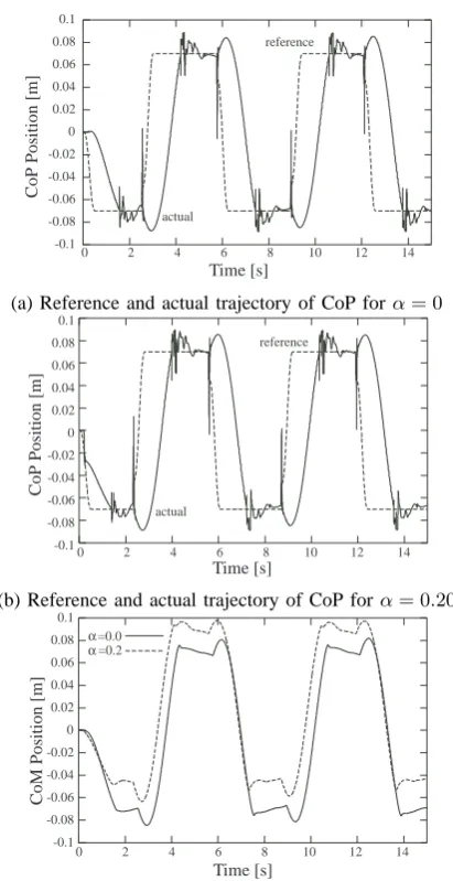
(a) Reference and actual trajectory of CoP forα= 0
-0.1 -0.08 -0.06 -0.04 -0.02 0 0.02 0.04 0.06 0.08 0.1
0 2 4 6 8 10 12 14
actual
reference
Time [s]
C
o
P
P
o
si
ti
o
n
[
m
]
(b) Reference and actual trajectory of CoP forα= 0.20
-0.1 -0.08 -0.06 -0.04 -0.02 0 0.02 0.04 0.06 0.08 0.1
0 2 4 6 8 10 12 14
α=0.0 α=0.2
Time [s]
C
o
M
P
o
si
ti
o
n
[
m
]
(c) Horizontal position of CoM.
Fig. 4. Simulation results.
IV. CONTROL FOR THESTEPPING MOTION BASED ON THEZMPFEEDBACK
In this study, a control method for stepping motion that is robust to an unknown constant external disturbance is considered. The control methods for the weight shift motion as well as the single leg static balance in the pre-vious section can be used in combination to automatically adjust the posture or motion with respect to the unknown external force and realize stepping motion using a simple biped robot. The main problem is how to switch the control law between the two schemes. Focusing on this aspect, we propose below a control method for stepping motion based on the ZMP (COP) information.
A. Control in double support phase
At the start of walking motion, the legs are on the ground in the double support phase. To take the first step, the weight has to be shifted to the supported side to prepare the other leg to become a swing leg. In this weight shift motion, the control method that is mentioned in the
section III is used where the reference CoP trajectory is tracked in a feedback control fashion. The body motion is modified as a result of this CoP control. The robot executes a weight shift motion by tilting the whole body so as to cope with a constant external force. Note that the CoP trajectory is adequately designed in advance so that the weight shift motion can be achieved.
B. Switching from double support phase
The control in the double support phase is based on the trajectory tracking control of the CoP position. When the CoP position becomes greater than a threshold value, the weight shift motion is regarded as sufficient. At this moment, the control law is switched from that for the double support phase to that for single support phase.
C. Control for single support phase
The static balance control law (17) is adopted to the ankle joint in the single support leg. In this phase, the body as well as the swing leg moves to perform the stepping motion according to the reference trajectories, which disturb the balance in this phase. However, this disturbance will be compensated by the control law (17). To generate the body and swing leg movements for stepping motion, the reference trajectories must be pro-vided for the feedback control of the two hip joints. For the adaptive motion, the reference trajectories must change with respect to the environment such as the slope angle. Therefore, the initial and end posture in the reference trajectory is produced, such that, the posture of the end of the double support phase is set as both an initial posture and a final posture. These two postures are interpolated continuously to achieve the lifting-up motion of the swing leg, i.e., the hip joint in the support leg are extended and then flexed in a constant amount.
D. Switching from single support phase
When the foot of the swing leg is placed on the ground, the control law is switched back to that for the double support phase.
E. Simulation
The control method in the previous section is simu-lated under the influence of the constant external force expressed as the following equations.
Fx=−M gsinα (50)
Fy=−M g(1−cosα). (51)
These external forces are equivalent to a set of external forces acting on the biped robot on the slope with slope angle α. The cases whereα= 0[rad] (no external force) and α = 0.2[rad] are examined. Parameters are: M = 2.5[kg],m = 1.25[kg], mf = 0[kg], L= 0.20[m], ` =
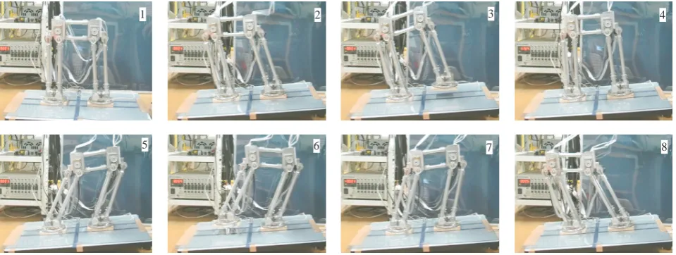
1 2 3 4
5 6 7 8
Fig. 5. In-place stepping motion experiment of the slope.
In the single support phase, the conventional PD control with nonlinear compensation is applied to the hip joints. These feedback gains are set toKd = 500andKp= 100. The graphs in Fig. 4(a) and (b) represent the time based plot of the CoP (ZMP) position. Regardless of the external forces, the similar CoP profile are obtained, implying that the weight shift is achieved as intended in both cases. The time based plot of the horizontal position of CoM is denoted in Fig. 4(c). It can be seen from the figure that when the external force is exerted, the stepping motion is performed such that the biped robot tilts the whole body against it.
V. EXPERIMENT
A. Apparatus
The reduced degree of freedom biped robot, whose design is originally proposed by Yoneda et al. [21], is used in experiments. This robot has parallel link structure in the leg parts as well as the body part, which keeps the soles parallel to each other. The biped robot is about 40[cm] in height and is about 2.9[kg] in weight. The sole is 12[cm] in length and the horizontal distance between right to left ankle is 20[cm]. Four motors are installed. One of them actuates the motion around yawing axis at ankle joints, which is not used in this experiment. The other three motors are used to achieve a stepping motion within the lateral plane.
A personal computer with RT-LINUX operating system is used to compute the torque output signal for all motors. The computed output signal is sent via D/A converter to the motor driver to make the motors generate the desired torque. A motion of the biped robot is detected by the rotary encoder installed in each motor. Three load cells are attached on each sole, from which the position of the CoP, i.e., ZMP is calculated. The controller’s sampling time is 1[ms] in this experiment.
B. Control law
The control law mentioned in the section IV was adopted. However, in the preliminary experiment, the biped robot tumbled in the single support phase. Thus, the control for ankle joint in the single support phase was changed from eq. (4) to the position control of the reference trajectory. The reference trajectory was set as follows. In the first 3[s], the ankle joint was extended 0.2[rad] from its initial value. The ankle kept the current angle during next 2[s] and then flexed 0.2[rad] to return to the initial angle in the next 3[s]. For the hip joints in the single support phase, on the other hand, the reference trajectories were set as follows. The hip joint of the support leg was extended 0.9[rad] in the first 5[s] and flexed 0.9[rad] in the next 5[s]. The reference trajectory of hip joint of the swing leg was generated based on the state of the support leg so that the two legs become almost parallel.
When the swing leg contacted with the ground, the control law was switched to that for the double support phase. Here, to ensure the ground contacts, the posture at the moment of the contact was kept for 1[s] before starting the control for the double support phase.
The control in the double support phase is the tracking control of the CoP position. The reference trajectory was set so that the CoP moved from the current position to 50mm away from the midpoint of the two ankle joints in 5[s]. The threshold value for switching to the one for single support phase was selected from the experiment and set at 38[mm] away from the mid point of the two ankle joints.
C. Results
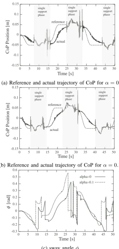
ground is shown in Fig. 6(a), while the one on the slope is shown in Fig. 6(b). Note here that, in the experiment, the CoP is not controlled in the shaded single support phase. Both CoP profiles of the two experimental conditions are not much different, implying that the stepping motion can be achieved regardless of the slope angle. The time based plot of the sway angleφis shown in Fig. 6(c). The profile of the slope condition is shifted up about 0.1 [rad] from that of the flat condition. This means that the biped robot realizes the stepping motion on the slope by tilting the whole body in the same amount as the slope angle. These results are consistent with the simulation results as shown in Fig.4
In the actual robot experiment, the control for ankle joint in the single support phase had to be changed from CoP feedback control to the conventional position feedback. One possible reason is the slow response of the control law (17) resulting in the inability to keep the balance with respect to the fast disturbances. Al-though the simulation results in section IV-E show that the response can be made faster with larger feedback control gains, large control gains in the actual biped robot induced mechanical vibration and the vibration impedes the control states to reach equilibrium points. The other significant reason is the mechanical problem. The slip due to wear at the set screw of the pulley is observed in the mechanical drive system of the hip joints. The slip led to control mismatch and, ultimately, loss of balance. As future works, we will fix the mechanical problem and re-examine the effectiveness of the original control law with CoP feedback in the single support phase.
VI. CONCLUSION
In this paper, a control method based on the ZMP feedback that allows the in-place stepping motion to be automatically adjusted according to the slope change is proposed. Using the fact that the ZMP and CoP is identical, the control method is constructed based on the CoP information detected using the force sensors on the sole. The invariance nature of the CoP reference trajectory with respect to the environmental conditions helps us construct a control law based on the CoP, i.e, ZMP feedback. This control method is basically constructed in combination with two control law: static balance control in the single support phase and weight shift movement in the double support phase. The effectiveness of the control law is confirmed by not only simulation results but also the empirical results. Consequently, the in-place lateral stepping motion is achieved on the slope as well as the flat ground without any modifications of the control law. However, the slow response in this control method as well as some mechanical matters become problems in the robot experiments, which should be improved in the future works.
REFERENCES
[1] M. Vukobratovic, B. Borovac, D. Surla, and D. Stokic, Biped Lo-comotion: Dynamics, Stability, Control and Application. Springer, 1990.
-0.15 -0.1 -0.05 0 0.05 0.1 0.15
0 5 10 15 20 25 30 35 40 45 50 Time [s]
C
o
P
P
o
si
ti
o
n
[
m
] reference
actual
single support phase
single support phase
single support phase
(a) Reference and actual trajectory of CoP forα= 0
-0.15 -0.1 -0.05 0 0.05 0.1 0.15
0 5 10 15 20 25 30 35 40 45 50 Time [s]
C
o
P
P
o
si
ti
o
n
[
m
] reference
actual
single support phase
reference
single support phase
single support phase
(b) Reference and actual trajectory of CoP forα= 0.1
-0.3 -0.2 -0.1 0 0.1 0.2 0.3 0.4 0.5 0.6
0 5 10 15 20 25 30 35 40 45 50 alpha=0
alpha=0.1
Time [s]
φ
[r
ad
]
(c) sway angleφ
Fig. 6. Experimental results.
[2] J. Yamaguchi and A. Takanishi, “Development of a Leg Part of a Humanoid Robot?Development of a Biped Walking Robot Adapting to the Humans’ Normal Living Floor,” Autonomous Robots, vol. 4, no. 4, pp. 369–385, 1997.
[3] K. Nagasaka, H. Inoue, and M. Inaba, “Dynamic walking pat-tern generation for a humanoid robot based on optimal gradient method,” Proc. of 1999 IEEE International Conference on Systems, Man and Cybernetics, vol. 6, 1999.
[4] K. Mitobe, G. Capi, and Y. Nasu, “Control of walking robots based on manipulation of the zero moment point,” Robotica, vol. 18, no. 06, pp. 651–657, 2001.
[5] S. Kagami, T. Kitagawa, K. Nishiwaki, T. Sugihara, M. Inaba, and H. Inoue, “A Fast Dynamically Equilibrated Walking Trajectory Generation Method of Humanoid Robot,” Autonomous Robots, vol. 12, no. 1, pp. 71–82, 2002.
[6] K. Hirai, M. Hirose, Y. Haikawa, and T. Takenaka, “The develop-ment of Honda humanoid robot,” Robotics and Automation, 1998. Proceedings. 1998 IEEE International Conference on, vol. 2, 1998. [7] Q. Huang, K. Kaneko, K. Yokoi, S. Kajita, T. Kotoku, N. Koyachi, H. Arai, N. Imamura, K. Komoriya, and K. Tanie, “Balance control of a biped robot combining off-line pattern with real-time modification,” Proc. of the 2000 IEEE International Conference on Robotics and Automation, vol. 4, pp. 3346–3352, 2000. [8] B. Lee, Y. Kim, and J. Kim, “Balance control of humanoid robot
for hurosot,” Proc. of IFAC World Congress, 200x.
[10] S. Kajita and K. Tani, “Experimental study of biped dynamic walking,” Control Systems Magazine, IEEE, vol. 16, no. 1, pp. 13–19, 1996.
[11] K. Nishiwaki, S. Kagami, Y. Kuniyoshi, M. Inaba, and H. Inoue, “Online generation of humanoid walking motion based on a fast generation method of motion pattern that follows desired ZMP,” IEEE/RSJ 2002 International Conference on Intelligent Robots and System, vol. 3, 2002.
[12] T. Sugihara, Y. Nakamura, and H. Inoue, “Real-time humanoid motion generation through ZMP manipulation based on inverted pendulum control,” Proceedings of 2002 IEEE International Con-ference on Robotics and Automation, vol. 2, 2002.
[13] S. Behnke, “Online Trajectory Generation for Omnidirectional Biped Walking,” Proceedings of IEEE International Conference on Robotics and Automation (ICRA 06), Orlando, Florida, pp. 1597–1603, 2006.
[14] D. Wollherr and M. Buss, “Posture modification for biped hu-manoid robots based on Jacobian method,” Proceedings. 2004 IEEE/RSJ International Conference on Intelligent Robots and Systems(IROS 2004), vol. 1, 2004.
[15] S. Napoleon and M. Sampei, “Balance control analysis of hu-manoid robot based on ZMP feedback control,” Proceedings of the 2002 IEEE/RSJ International Conference on Intelligent Robots and Systems, pp. 2437–2442, 2002.
[16] A. Goswami, “Postural Stability of Biped Robots and the Foot-Rotation Indicator (FRI) Point,” The International Journal of Robotics Research, vol. 18, no. 6, p. 523, 1999.
[17] P. Kulvanit, H. Wongsuwan, B. Srisuwan, K. Siramee, A. Boon-prakob, T. Maneewan, and D. Laowattana, “Team KMUTT: Team Description Paper,” Robocup 2005: Humanoid League, 2005. [18] S. Ito and H. Kawasaki, “Regularity in an environment produces
an internal torque pattern for biped balance control,” Biological Cybernetics, vol. 92, no. 4, pp. 241–251, 2005.
[19] S. Ito, H. Asano, and H. Kawasaki, “A balance control in biped double support phase based on center of pressure of ground reaction forces,” 7th IFAC Symposium on Robot Control, pp. 205– 210, 2003.
[20] S. Ito, S. Amano, M. Sasaki, and P. Kulvanitt, “In-place lateral stepping motion of biped robot adapting to slope change,” Pro-ceedings of the 2007 IEEE International Conference on Systems, Man and Cybernetics, pp. 1274–1279, 2007.
[21] K. Yoneda, T. Tamaki, Y. Ota, and R. Kuratsume, “Design of bipedal robot with reduced degrees of freedom,” Journal of the Robotics Society of Japan, vol. 21, no. 5, pp. 546–553, 2003.
Satoshi Ito received B. Eng. and M. Eng. Degrees in
infor-mation engineering from Nagoya University in 1991 and 1993, respectively. From 1994 to 1996, he was a technical staff at lab. for Bio-Mimetic Control Research Center (RIKEN) and from 1997 to 1999 a research scientist at this laboratory. In 1999, he received D. Eng. degree from Nagoya University. Since 1999, he has been with the faculty of Engineering, Gifu University. His research interests include the system control, robotics and mechatronics.
Shinya Amano received his M. Eng. degree in mechanical
system engineering from Gifu University, Japan, in 2007. He is currently with Aisin Seiki Co., Ltd.
Minoru Sasaki received M. Eng. and D. Eng. Degrees in
me-chanical engineering from Tohoku University in 1983 and 1985, respectively. He was a research associate at Tohoku University in 1985 and a lecturer at Miyagi National College of Technology, and a visiting professor at the University of California, Los Angeles. From 1991, he has been with Faculty of Engineering, Gifu University and is currently a professor. His current research interests include the control theory, mechatronics and intelligent control.
Pasan Kulvanit received MS degree from the University of