Published online October 15, 2014 (http://www.sciencepublishinggroup.com/j/ajae) doi: 10.11648/j.ajae.s.2015020101.16
Computational investigation of aerodynamic characteristics
and drag reduction of a bus model
Eyad Amen Mohamed
*, Muhammad Naeem Radhwi, Ahmed Farouk Abdel Gawad
Mech. Eng. Dept., College of Eng. & Islamic Archit., Umm Al-Qura Univ., Makkah, Saudi ArabiaEmail address:
eytworld@gmail.com (E. A. Mohamed), mnradhwi@uqu.edu.sa (M. N. Radhwi), afaroukg@yahoo.com (A. F. A. Gawad)
To cite this article:
Eyad Amen Mohamed, Muhammad Naeem Radhwi, Ahmed Farouk Abdel Gawad. Computational Investigation of Aerodynamic Characteristics and Drag Reduction of a Bus Model. American Journal of Aerospace Engineering. Special Issue: Hands-on Learning Technique for Multidisciplinary Engineering Education. Vol. 2, No. 1-1, 2015, pp. 64-73. doi: 10.11648/j.ajae.s.2015020101.16
Abstract:
It is well-known that buses comprise an important part of mass transportation and that there are many types of buses. At present, the bus transportation is cheaper and easier to use than other means of transportation. However, buses have some disadvantages such as air pollution due to engine exhaust. This study is an attempt to reduce the gas emissions from buses by reducing the aerodynamic drag. Several ideas were applied to achieve this goal including slight modification of the outer shape of the bus. Thus, six different cases were investigated. A computational model was developed to conduct this study. It was found that reduction in aerodynamic drag up to 14% can be reached, which corresponds to 8.4 % reduction in fuel consumption. Also, Neuro-Fuzzy technique was used to predict the aerodynamic drag of the bus in different cases.Keywords:
Computational Investigation, Aerodynamic Characteristics, Drag Reduction, Bus Model1. Introduction
1.1. Background
Nowadays, the waste of energy and the environmental pollution are some of the major global concerns for all science disciplines especially engineering. There are a lot of researchers who studied the aerodynamic behavior around heavy vehicles and tried to control their harmful emissions. Thus, they considered how to find out a better way to improve the vehicle performance by modifying the shape and weight of the vehicle.
Buses are one type of the heavy vehicles that consume much fuel. They are road vehicles designed to carry passengers in different applications. Buses can have a capacity as high as 300 passengers. The most common type of buses is the single-decker rigid bus. The larger loads are carried by double-decker buses and articulated buses. The smaller loads are carried by midi-buses and minibuses. Coaches are used for longer distance services.
Bus manufacturing is increasingly globalised with the same design appearing around the world. Buses may be used for scheduled bus transport, scheduled coach transport, school transport, private hire, tourism, etc. Promotional buses may be used for political campaigns and others are privately operated for a wide range of purposes.
Historically, Horse-drawn buses were used from the 1820s, followed by steam buses in the 1830s, and electric trolleybuses in 1882. The first internal combustion engine buses were used in 1895 [1]. Recently, there has been growing interest in hybrid electric buses, fuel cell buses, electric buses as well as ones powered by compressed natural gas or bio-diesel.
1.2. Previous Investigations
Generally, there is somehow shortage in the investigations that consider aerodynamics of buses in comparison to other heavy vehicles, e.g., trucks.
Newland [1] aimed to develop a transit bus fuel consumption function based upon relationships found in the literature between bus fuel consumption and various bus operating characteristics especially their variable passenger loads.
Roy and Srinivasan [2] studied the aerodynamics of trucks and other high-sided vehicles that are of significant interest in reducing road accidents due to wind loading and in improving fuel economy. They concentrated on the associated drag due to the exterior rear-view mirrors. They stated that modifying truck geometry can reduce drag and improve fuel economy.
American Journal of Aerospace Engineering 2015; 2(1-1): 64-73 65
of trucks, buses, motor homes, reentry vehicles, and other large-scale vehicles. They presented preliminary results of both the effort to formulate a new base drag model and the investigation into a method of reducing total drag by manipulating forebody drag.
Yamin [4] used computational fluid dynamics (CFD) technique to simulate external flow analysis of a coach. His results suggested that the steady state CFD simulation can be used to boost the aerodynamic development of a coach.
Abdel Gawad and Abdel Aziz [5] investigated experimentally and numerically the effect of front shape of buses on the characteristics of the flow field and heat transfer from the rear of the bus in driving tunnels. Their study covered three bus models with flat-, inclined-, and curved-front shapes. They found that the front shape of the bus affects its aerodynamic stability in driving tunnels. Also, they stated that the cooling of the inclined- and curved-front vehicles is better than the cooling of the flat-front bus by about 20%.
François et al. [6] studied experimentally the aerodynamics characteristics and response of a double deck bus, which is a bus type very used in the Argentinean routes, submitted mainly to cross-wind. They measured pressure distributions over the frontal and lateral part of the bus and also drag and lateral forces related to the position of centre of gravity.
Yelmule and Kale [7] considered experimentally and numerically the aerodynamics of open-window buses where airflow due to motion provides comfort. They stated that an overall drag reduction of about 30% at 100 km/h can be reached by modifying the bus exterior body.
Mohamed-Kassim and Filippone [8] analyzed the fuel-saving potentials of drag-reducing devices retrofitted on heavy vehicles. They considered realistic on-road operations by simulating typical driving routes on long-haul and urban distributions; variations in vehicle weight. Their results show that the performance of these aerodynamic devices depend both on their functions and how the vehicles are operated such that vehicles on long-haul routes generally save twice as much fuel as those driven in urban areas.
Patil [9] performed aerodynamic flow simulation on one of conventional bus to demonstrate the possibility of improving the performance with benefits of aerodynamic features around the bus by reducing drag, which improves the fuel consumption. They optimized one of the conventional bus models and tried to reduce drag by adding spoilers and panels at rear portion along with front face modification. Their results showed that drag can be decreased without altering the internal passenger space and by least investment.
Also, the issue of fuel consumption was covered by many authors [10] and [11].
1.3. Present Investigation
The present study focuses on the aerodynamic characteristics of buses especially drag, either form or friction, which influences directly the fuel consumption.
A computational model was developed using the commercial code ANSYS-Fluent 13 to predict the aerodynamic performance of buses.
Modifications of the external body and/or surface of the bus to reduce the aerodynamic drag are proposed. The authors carefully considered that the proposed modifications do not affect the safety and operation of the bus. Also, the modifications do not change the main body/structure of the bus. Actually, modifications can be applied with considerably low cost and fairly technical skills.
The computations were carried out for different values of Reynolds number.
2. Governing Equations and Turbulence
Modeling
2.1. Governing Equations
The equations that govern the fluid flow around a model are time-averaged continuity and momentum equations which, for the steady, incompressible flow, are given by, respectively:
= 0 i =1, 2, 3 (1)
U = ν − u u −
ρ
i,j =1,2, 3. (2)
In the above, Ui is the mean-velocity vector with
components U, V and W in x, y and z directions, respectively,
P is the static pressure, ρ is the fluid density and is its kinematic viscosity. Repeated indices imply summation. The turbulence model involves calculation of the individual Reynolds stresses ( ) using transport equations. The individual Reynolds stresses are then used to obtain closure of the Reynolds-averaged momentum equation (Eq. 2).
2.2. Turbulence Modeling (Realizable k- ɛ Turbulence Model)
The realizable k-ɛ turbulence model was used in the present study. The realizable k-ɛ model differs from the standard k-ɛ model in two important ways:
• The realizable k-ɛ model contains an alternative formulation for the turbulent viscosity.
• A modified transport equation for the dissipation rate,
ɛ, has been derived from an exact equation for the transport of the mean-square vorticity fluctuation. For further details about the realizable k-ɛ turbulence model, one may refer to [12].
2.3. Drag Calculations
The results focus on the drag coefficient, i.e., pressure (form), friction, and total drag coefficients.
2.3.1. Pressure (form) Drag
The coefficient of pressure drag, , is calculated by Eq. 3 as follows,
= ( ."×$×∆
%&) (3)
() = × 0.5 # + # ,-. # /0
Where, Dp is the drag force due to pressure,
(projected) area of the bus = H × W, ρ is the the bus speed, and ∆P is the pressure difference
front and rear surfaces of the bus.
2.3.2. Friction Drag
The force of friction drag is calculated surfaces and roof of the bus using the following
(1 = 1#.+ # ,-. ∗ /34
Where, 1 is the coefficient of friction area summation of roof and side surfaces = roof area = L × W, and AS is the side surfaces
Generally, the actual operating Reynolds
L /ν) is greater than the critical Reynolds number 105 for a flat surface) for all test cases, which
is turbulent. Thus, the coefficient of friction as [13]:
1= . 5
367
8
9
Where, L is the bus length and ν is the viscosity.
2.3.3. Total Drag
The value of the total drag force, (:, is calculated
(: (); (1
Then, the coefficient of total drag, :, is
: = <=
."#$# %&'>?
3. Original and Modified Models
The original model represents an actual produced by Mercedes Benz, Type: Coach Fig. 1.
Figure 1. Side view of the bus [14].
This original model is considered as reference of the present study. The total length 13 m, the width is 2.55 m, and the height shown in Fig. 1. The fuel tank capacity is about
Some modifications were proposed to the Each modification produced a new model. was given to each new model for classification. the names and shapes of the different models.
(4)
pressure, AF is the frontal
flow density, U∞ is difference between the
calculated for the two side following equation:
(5)
friction drag, ARS is the = AR + AS, AR is the
surfaces = 2 × L × H. Reynolds number (Re = U∞
number (Recr = 5 × which means the flow friction drag is calculated
(6)
the flow kinematic
calculated as:
(7)
is calculated as:
(8)
Models
actual bus that was Coach Travego M [14],
[14].
as the comparing length of the bus is height is 3.1567 m as
about 475 litres. the original model. model. A specific name classification. Table 1 shows
models.
Table 1. Names and shapes
No. Name View
1 Original
2 MCOBS1
3 MCOBS2
4 MCOBS3
5 MCOBS4
6 MCOBS5
7 MCOBS6
The names and shapes that explained as follows:
Original: It is the actual modifications.
MCOBS1: A curved device is direct the air flow downward directly two supports.
MCOBS2: Similar to MCOBS1
shapes of the different models
that appear in table 1 can be
shape of the bus without
is added at the rear of the bus to directly behind the bus. It has
American Journal of Aerospace Engineering 2015; 2(1-1): 64-73 67
and right ends of the curved device to grantee that all air is directed downward without side escape.
MCOBS3: The bus is equipped with the same device of MCOBS2. Also, two small ducts (4500×50×300mm) are added on both sides of the bus to drive air, with relatively high pressure, to the low-pressure zone behind the bus.
MCOBS4: Only two small ducts are added on both sides of the bus. There is no curved device.
MCOBS5: The bus is equipped with a curved device similar to MCOBS1. The front surface of the bus is modified to have a suitable curvature.
MCOBS6: Similar to MCOBS5 but the rear surface has also a curvature similar to the one of the front surface.
4. Computational Aspects
4.1. Tested Velocities
The computations were mainly carried out at 100 km/h (27.22 m/s) for all cases. However, to evaluate the effect of bus velocity on the aerodynamic characteristics and drag, other three values of velocity were examined for the case of MCOBS5. Table 2 shows the four values of velocity and the corresponding values of Reynolds number.
Table 2. Tested bus velocities.
NO. Speed (Km/h) Speed (m/s) Reynolds number
1 70 19.44 16.73 × 10⁶
2 100 27.22 23.9 × 10⁶
3 120 33.33 28.68 × 10⁶
4 150 41.66 35.85 × 10⁶
4.2. Computational Domain and Boundary Conditions
As seen in Figure 2, the computational domain is a rectangle that contains the bus. The dimensions of the domain were selected to ensure free development of the air flow around the bus.
The boundary conditions of the domain can be listed as: (i) Uniform velocity at the inlet surface. (ii) Zero pressure-gradient at the outlet surface. (iii) Solid condition at the ground, i.e., the surface below the bus. (iv) Symmetry condition at the two side surfaces and the top surface of the domain.
Figure 2. Computational domain and boundary conditions.
4.3. Computational Grid (Mesh)
The computational domain was discretized using unstructured grids. This type of grids usually guarantees the flexibility of generating enough computational points in locations of severe gradients. The computational domain was covered with tetrahedral elements (Figure 3). The grid is very fine next to the solid boundary. The dimensionless distance between the wall and first computational point is y+ ≈ 1.8, which is calculated as
y+ = @AC B (9)
Where, y is the distance to the first point off the wall, ν is the kinematic viscosity, D is the friction velocity.
D= E$D,
τ
is the wall shear stress and ρ is the flow density. The value of y+≈ 1.8 ensures good resolution of the complexturbulent flow.
(a) Grid structure for "Original" shape.
(b) Grid structure for MCOBS1.
(c) Grid structure for MCOBS6.
Figure 3. Samples of grid structures.
4.4. Grid Independency
Careful consideration was paid to ensure the grid-independency of the computational results. Therefore, three grid sizes were used to test the grid-independency, namely: 50,000, 65,000 and 85,000 elements (cells).
difference between the results of the second and third grids is in the range of 2-3%. Thus, the second grid size (65,000) was used for all test cases.
4.5. Numerical Scheme
SIMPLE algorithm (Semi-Implicit Method for
Pressure-Linked Equations) was used to solve the velocity and pressure fields. Each momentum equation was solved by the ‘’ first-order upwind’’ scheme.
The ‘’standard wall function’’ was used as the near-wall technique in the turbulence model. The solution continues until the numerical error of all computed quantities gets below 10-5.
4.6. Validation of the Present Computational Algorithm
The present numerical result of the total drag coefficient
F= 0.698 for the ‘’original’’ compares very well to the range of 0.6-0.8 that was reported in [13]. The present value of F lies exactly in the middle of the range. This gives confidence in the present computational scheme.
5. Results and Discussions
This section shows the computational results of the different considered cases (Original and modified models) that were mentioned in Sec.3. The main objective is to find the modified model that gives maximum drag reduction. However, the flow field (pressure and velocity) around the bus model is illustrated.
5.1. Investigated Cases
As it is well-known, the pressure (form) drag represents the major part of the total drag on bus in comparison to the friction drag, the pressure distributions on the frontal and rear surfaces are considered. The pressure drag depends on the difference between the pressure distributions on the frontal and rear surfaces of the bus. Figures 4 and 5 illustrate the pressure contours on the frontal and rear surfaces of the bus, respectively, for all cases.
The velocity field in the zone adjacent to the rear surface affects the pressure distribution on rear surface. Thus, velocity vectors, in a vertical section, are shown in Figure 6 for all cases. The vertical section passes through the mid-section of the bus width.
The results of various cases are discussed as follows:
5.1.1. Original
As expected, Figures 4 and 5 show that the pressure is really high on the bus frontal surface due to flow stagnation. The pressure is very low on the rear surface due to wake formation behind the bus. Figure 6 shows that two main vortices are formed in the wake zone behind the bus. The two vortices have nearly equal size. For this case, at Re = 23.9 × 10⁶, the total drag coefficient ( F) equals 0.698.
5.1.2. Mcobs1
As can be seen in Figure 5, the curved-surface device at the rear of the bus reduces slightly the pressure on the rear surface in comparison to the ‘’Original ‘’. However, this change of pressure does not considerably reflect on the value of F that becomes 0.649.
Another effect of the curved-surface device is seen in Figure 6. The upper vortex behind the bus becomes smaller then the lower vortex. The curved-surface device directed the flow from the top surface at the bus to the wake zone behind the bus.
Figure 4. Pressure contours on the frontal surface.
Origin al MCOBS1
MCO BS2 MCOBS3
MCOBS4 MCOBS5 100Km/h
MCOBS5 70Km/h MCOBS5 120Km/h
American Journal of Aerospace Engineering 2015; 2(1-1): 64-73 69
Figure 5. Pressure contours on the rear surface.
Original MCOBS1
MCOBS2 MCOBS3
MCOBS4 MCOBS5 100km/h
MCOBS5 70km/h MCOBS5 120km/h
MCOBS5 150km/h MCOBS6
Figure 6. Velocity vectors behind the bus in a vertical section.
5.1.3. Mcobs2
It seems that the closed ends of the curved-surface device
Original MCOBS1
MCOBS2 MCOBS3
MCOBS4 MCOBS5 100Km/h
MCOBS5 70Km/h MCOBS5 120Km/h
have a minor effect on the pressure distributions, Figure 5. In Figure 6, the vortices behind the bus are altered in comparison to MCOBS1. The value of F is 0.652, which is very close to that of MCOBS 2. Thus, the curved-surface device reduces the value at Fin comparison to the ‘’Original’’.
5.1.4. Mcobs3
It seems that the two side ducts have a negative effect to the curved-surface device. They do not help in reducing the total drag on the bus. Unfortunately, they increase the value of F to reach 0.691, which is greater than the two values of MCOBS1 ( F= 0.649) and MCOBS2 ( F= 0.652). However, it is slightly lower than the value at the ‘’original’’ ( F= 0.698).
This may be attributed to the long path of the ducts, which causes big pressure drop inside them. Thus, air may be ever sucked inside them at their rear ends causing increase in the value of F. Generally, it is clear from Figure 6 that there is almost no change in comparison to MCOBS2.
5.1.5. Mcobs4
It is obvious that the two ducts alone have no effect in reducing the total drag on the bus. The value at F is 0.697, which is the same as the ‘’Original’’ ( F=0.698). However, the two ducts cause the lower vortex behind the bus to extend downstream, Figure 6.
5.1.6. Mcobs5
It is found that the curvature at the frontal surface causes a noticeable change on the total drag on the bus. Thus, the value of F becomes 0.632 for 100 km/h. This value is lower than that of the ‘’Original’’ ( F=0.698).
In Figure 6, as expected, the curvature at the frontal surface has no effect on two vortices in the wake region behind the bus.
5.1.7. Mcobs6
It is obvious that the curvatures of the frontal and rear surfaces cause a remarkable change on pressures of these two surfaces, Figures 4 and 5. Thus, the value of F reduces to 0.602.
This is the lowest value of F achieved in all test cases. Also, the wake zone behind the bus is favorably changed as can be seem in Figure 6.
5.2. Overall view of all cases
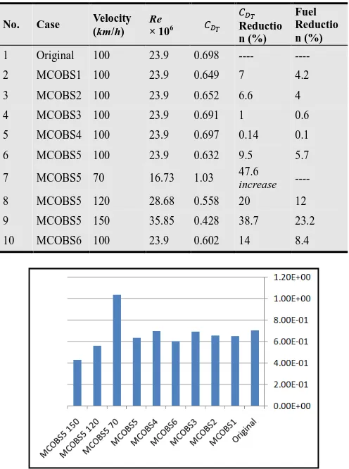
Based on the results of the previous section, an overall view of all cases can be demonstrated. Table 3 illustrates overall results of the total drag coefficient ( F) for all cases. Also, Figure 7 shows the values of total drag coefficient ( F) for all cases. Moreover, table 3 illustrates the percentage reduction in total drag coefficient for all cases of bus modifications.
It is clear from Table 3 and Figure 7 that the lowest value of
F = 0.602, which corresponds a total drag reduction of 14%, is obtained for case MSCOBS6. This is the case of modifying the frontal and rear surfaces by slight curvature. This is the best case.
Whereas, the worst case is MCOBS4 with F = 0.697 and total drag reduction of 0.14%.
Thus, the idea of putting two side ducts seems useless. This is may be attributed to the relatively big length of the ducts. Internal friction at the walls of the ducts causes considerable pressure loss inside them. Thus, there is no pressure rise by the end of the ducts at the rear surface of the bus.
Table 3. Overall results of F.
No. Case Velocity (km/h) Re × 106 F
F
Reductio n (%)
Fuel Reductio n (%)
1 Original 100 23.9 0.698 ---- ----
2 MCOBS1 100 23.9 0.649 7 4.2
3 MCOBS2 100 23.9 0.652 6.6 4
4 MCOBS3 100 23.9 0.691 1 0.6
5 MCOBS4 100 23.9 0.697 0.14 0.1
6 MCOBS5 100 23.9 0.632 9.5 5.7
7 MCOBS5 70 16.73 1.03 47.6
increase ----
8 MCOBS5 120 28.68 0.558 20 12
9 MCOBS5 150 35.85 0.428 38.7 23.2
10 MCOBS6 100 23.9 0.602 14 8.4
Figure 7. Values of total drag coefficient ( F) for all cases.
Table 4. An example of fuel saving
Fuel consumption of ‘’Original’’ (Liter/h)
Percentage fuel saving (%) MOCBS6
Fuel consumption of MOCBS6 (Liter/h)
Fuel saving (Liter/h) MOCBS6
66.88 8.4 61.26 5.618
Also, Table 3 indicates that a considerable drag reduction up to 38.7%, at 150 km/h, can be reached by increasing the bus velocity. This drag reduction may be attributed to the separation delay or even prevention due to the high momentum of the air surrounding the bus.
Unfortunately, high velocities are not always practical due to traffic and safely considerations. In table 3, the fuel reduction percentage was calculated based on the approximate relationship that was derived from [15]:
Fuel reduction %= (3/5) × Total drag reduction % (10)
American Journal of Aerospace Engineering 201
annual saving of an intercity bus that operates velocity of 100 km/h.
6. Adaptive Neuro-Fuzzy Inference
System (ANFIS)
6.1. Introduction
The Adaptive Neuro-Fuzzy Inference system used to predict the values of the pressure drag based on the obtained data from the investigation. A well-trained nruro-fuzzy scheme the prediction successfully based on enough data. After training, this technique enables new values of F that were not predicted computational study. Application of ANFIS programming effort and computer run-time traditional computational fluid dynamics (CFD
Fuzzy logic (FL) is a form of many-valued deals with reasoning that is approximate rather exact. Compared to traditional binary sets may take on true or false values), fuzzy logic have a truth value that ranges in degree between
ANFIS is a kind of neural network
Takagi–Sugeno fuzzy inference system. Since both neural networks and fuzzy logic potential to capture the benefits of both in a Its inference system corresponds to a set of rules that have learning capability to approximate functions. Hence, ANFIS is considered
estimator.
For more details about ANFIS, one may and [17].
6.2. Present ANFIS Model
Table 5. Training data for all cases
Case
Input
Code Reynolds number
Original 1 23.9 × 10⁶
MCOBS1 2 23.9 × 10⁶
MCOBS2 3 23.9 × 10⁶
MCOBS3 4 23.9 × 10⁶
MCOBS4 5 23.9 × 10⁶
MCOBS6 6 23.9 × 10⁶
MCOBS5 7 23.9 × 10⁶
MCOBS5-70 8 16.73 × 10⁶
MCOBS5-120 9 28.68 × 10⁶
MCOBS5-150 10 35.85 × 10⁶
ANFIS was constructed based on "Quadrangle
The two input parameters to ANFIS are the Reynolds number (Re). The bus cases are coded
American Journal of Aerospace Engineering 2015; 2(1-1): 64-73
operates at an average
Inference
system (ANFIS) was drag coefficient F
the computational scheme can perform enough computational enables the prediction of predicted by the
ANFIS needs much less
time in comparison to
CFD) techniques.
valued logic, which rather than fixed and sets (where variables logic variables may between 0 and 1.
that is based on Since it integrates principles, it has single framework. of fuzzy IF–THEN approximate nonlinear to be a universal
refer to Refs. [16]
cases
Output Pressure drag coefficient (LMN) 0.661 0.611 0.614 0.654 0.564 0.659 0.595 0.994 0.522 0.392 "Quadrangle prediction". the bus case and the coded as numbers,
Table 5.
The output of ANFIS is the pressure Table 5 shows the training data
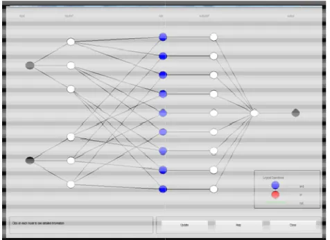
Figures 8 and 9 illustrate performance surface of ANFIS, the variation of the Quadrangle (bus case and Re), which end up
After the success in training ANFIS was not seen before by the ANFIS output ( ).
Thus, the ability of ANFIS to as output is confirmed. Table 6 shows the new corresponding predictions of output.
Figure 8. Structure of ANFIS model
Figure 9. Output surface of performance
Prediction).
Figure 10 represents validation Comparison is made between the (Red) and the corresponding ANSYS-Fluent scheme (Blue) as
Generally, it is clear that there
ANFIS and CFD predictions. The
predictions may be attributed mainly small number of cases (10) that The generality of ANFIS that considered bus with modifications. Better
71
pressure drag coefficient ( ). for all cases.
illustrate the structure and output respectively. Figure 9 explains predictions with the two inputs up with convergence.
ANFIS, new set of data, which
ANFIS, is introduced to predict
to predict correctly the values of
set of input data and the output.
model (Quadrangle Prediction).
performance of ANFIS model (Quadrangle
validation of ANFIS new predictions. the new predictions of ANFIS corresponding predictions of the present
as CFD results.
ANFIS is modeled for each bus case with different values of Re.
However, Figure 10 suggests that ANFIS technique is promising if the above two points are carefully considered.
Table 6. Prediction of new data.
Input Output
Code Reynolds number Pressure drag coefficient (L
MN)
1 23.6 × 10⁶ 0.621
2 20.1 × 10⁶ 0.64
3 19.1 × 10⁶ 0.902
4 22.4 × 10⁶ 0.794
5 23.0 × 10⁶ 0.757
6 18.7 × 10⁶ 1.45
7 27.1 × 10⁶ 0.691
Figure 10. Validation of ANFIS new data.
7. Conclusions
A computational scheme was developed to study the possibility of drag reduction of buses. An actual bus was chosen to carry out the study. The values of the total drag coefficient C(DT), corresponding to suggested modifications
to the bus, were computed. Seven case studies were investigated and the reductions in total drag and fuel were recorded.
Based on the results and discussions of the previous sections, the following concluding points can be stated:
1. The curvature modification of the frontal and rear surfaces, case MCOBS6, gives the best drag reduction of 14%. This gives a consequence fuel savings of about 8.4%.
2. The proposed curvature at the frontal and rear surfaces is accepted from the economic and manufacturing points of view. This modification is easy to be implemented as it does not affect the body/structure of the bus.
3. The idea of adding a rear curved–shape device seems interesting. The present curved–shape causes a maximum drag reduction of 7 %, which corresponds to a fuel saving of about 4.2 %.Perhaps introducing
other profiles of the curved-shape is a good idea to find the optimum profile that gives the highest drag reduction.
4. The using of side ducts proved to be inefficient technique. The idea of transferring high pressure from the upwind zone of the bus to its downwind zone to increase the pressure at the rear surface of the bus did not succeed. This may be attributed to the relatively big length of the ducts. Thus, internal friction causes losses and overall pressure drops in the ducts. So, the pressure at the rear surface of the bus is nearly the same as that of the bus wake.
5. The total drag on the bus decreases with the bus speed. However, the considerations of traffic and safety limit this option of increasing the bus speed.
6. Although the maximum value of fuel saving of 8.4% at 100 km/h of the present study is not a big number, it represents a very good achievement when considering the huge amount of fuel consumption of buses allover the world, e.g., intercity buses.
7. Fairly good predictions were obtained from ANFIS. Increasing the amount of training data will certainly improve its efficiency.
8. Other ideas may be considered in future investigations such as:(i) air jets, using a suitable pneumatic system, may be injected from the rear surface of the bus to increase the pressure in the wake zone. (ii) Minimizing flow separation by tapering or rounding the fore-body of the bus, and modifying the roof of the bus.
Nomenclature
AF : Frontal area.
/4 : Side area = 2×L×H. /3 : Roof area =L × W. / 34 = /3 +/4 .
1 : Friction drag coefficient. ) : Pressure drag coefficient. : : Total drag coefficient. ) : Pressure coefficient. (1 : Frictions drag force (N). () : Pressure drag force (N). (: : Total drag force (N). H : Bus height.
L : Bus length.
P : Pressure (kPa).
OP : Outlet pressure (kPa). Re : Reynolds number.
QRST : Critical Reynolds number for flow on a flat plat. ,∞ : Bus velocity.
W : Bus width.
American Journal of Aerospace Engineering 2015; 2(1-1): 64-73 73
Abbreviations
ANFIS : Adaptive Neuro-Fuzzy Inference system
CFD : Computational fluid dynamics.
FL : Fuzzy logic
GRV : Ground research vehicle.
SIMPLE : Semi-Implicit Method for Pressure-Linked
Equations.
References
[1] L. E. Newland, "A Fuel Consumption Function for Bus Transit Operations and Energy Contingency Planning", Technical Report: UM-HSRI-80-53, Highway Safety Research Institute, The University of Michigan, July 1980.
[2] S. Roy, and P. Srinivasan, ”External Flow Analysis of a Truck for Drag Reduction’’, International Truck and Bus Meeting & Exposition, Paper #: 2000-01-3500, 2000.
[3] C. Diebler and M. Smith, "A Ground-Based Research Vehicle for Base Drag Studies at Subsonic Speeds", Technical Report: NASA/TM-2002-210737, NASA Dryden Flight Research Center, Edwards, California, November 2002.
[4] A. K. M. Yamin, "Aerodynamic Study of a Coach Using Computational Fluid Dynamic (CFD) Technique", M.Sc. in Automotive Engineering, Faculty of Engineering and Computing, Coventry University, August 2006.
[5] A. A. Abdel Aziz, and A. F. Abdel Gawad, “Aerodynamic and Heat Transfer Characteristics around Vehicles with Different Front Shapes in Driving Tunnels,” Proceedings of Eighth International Congress of Fluid Dynamics & Propulsion (ICFDP 8), December 14-17, 2006, Sharm El-Shiekh, Sinai, Egypt.
[6] D. G. François, J. S. Delnero, J. Colman, Di Leo J. Marañón and M. E. Camocardi, "Experimental determination of Stationary Aerodynamics loads on a double deck Bus", 11th Americas Conference on Wind Engineering, San Juan, Puerto Rico, June 22-26, 2009.
[7] M. M. Yelmule and S. R. Kale, ’’Aerodynamics of a Bus with Open Windows’’, Int. J. Heavy Vehicle Systems, Vol. 16, No. 4, 2009.
[8] Z. Mohamed-Kassim, A. Filippone, "Fuel savings on a heavy vehicle via aerodynamic drag reduction", Transportation Research Part D 15, 275-284, 2010.
[9] C. N. Patil, K.S. Shashishekar, A. K. Balasubramanian, and S. V. Subbaramaiah, "Aerodynamic Study and Drag Coefficient Optimization of Passenger Vehicle", International Journal of Engineering Research & Technology (IJERT), Vol. 1, Issue 7, September-2012.
[10] Bob Lloyd, "Dissecting the Basic Fuel Consumption Equation into Its Components to Improve Adaptability to Changing Vehicle Characteristics", 25th ARRB Conference-Shaping the Future: Linking Policy, Research and Outcomes, Perth, Australia, 2012.
[11] I. M. Berry, "The Effects of Driving Style and Vehicle Performance on the Real-World Fuel Consumption of U.S. Light-Duty Vehicles", M.Sc. Mechanical Engineering and M.Sc. Technology and Policy, Massachusetts Institute of Technology, February 2010.
[12] Fluent guide manual, (2011).
[13] F. M. White, "Fluid Mechanics", McGraw-Hill, 7th Edition, 2008.
[14] Mercedes-Benz, Reisebus/Coach Travego M, Mannual. http://ebookbrowsee.net/1843659-graphics-travego-pdf-d9474 9039
[15] J. Patten, B. McAuliffe, W. Mayda, and B. Tanguay, ‘’Review of Aerodynamic Drag Reduction Devices for Heavy Trucks and Buses’’ NRC-CNRC Technical Report, Canada, 2012.
[16] Matlab guide manual, 2011.
![Figure 1. Side view of the bus [14].[14].](https://thumb-us.123doks.com/thumbv2/123dok_us/8572233.1716950/3.595.45.294.565.654/figure-view-bus.webp)