1. Introduction
Composite materials are growingly being used in many engineering applications due to their strength, stiffness, and lightness. Among their types, composites with multilayers are the mostly used because of their firmness against thermal and mechanical loads. As a conventional layered composite, the layers are usually structured from ceramics and metal. Due to the distinct interface between ceramic and metallic layers, material properties across the interface undergo a sudden change, which produces stress jump and may give a rise to delamination or cracking of the interface. To overcome this shortage, a new technique of grading between ceramic and metal layers was developed by Japanese material scientists in 1984 [1]. Materials with the mentioned grading are called Functionally Graded Materials (FGMs), which are heat-resisting by ceramic, and fracture-resisting by metal with smooth graded transition of material properties.
Along various applications, new methodologies for predicting FGMs’ mechanical and thermal behavior have been developed. Chakraborty et al. [2] presented a beam element to study free vibration and wave propagation in laminated composite beam structures with symmetric as well as asymmetric ply stacking. Chakraborty et al. [3] developed a beam element to study the thermoelastic behavior of FGM beams based on the first-order shear deformation theory. Static, free vibration and wave propagation problems were considered. Vallejo et al. [4] introduced a new absolute nodal
Finite Element Coding of Functionally Graded Beams under
Various Boundary and Loading Conditions
Othman Al-Hawamdeh
, Ibrahim Abu-Alshaikh, Naser Al-Huniti
Department of Mechanical Engineering, University of Jordan, Amman-11942, Jordan.A B S T R A C T P A P E R I N F O
Detailed formulation and coding of exact finite element is carried out to study the static behavior of a layered beam structure. The beam element is modelled based on the first-order shear deformation theory and it is assumed to be composed of three layers whereas the middle layer is made of functionally graded material (FGM), i.e. with variable elastic properties in the thickness direction. The shape of the FGM mechanical properties variation in the thickness direction takes the form of exponential or power-law. The governing equations and boundary conditions are derived by applying the virtual work principle. Variations of displacements along the beam and stresses across the depth due to mechanical loadings are investigated. Comparative examples are carried out to highlight the static behavior difference between FGM layered beams and pure metal-ceramic beams.
Chronicle:
Received: 21 June 2017 Accepted:30 September 2017
Keywords :
Beam Structure.
Shear Deformation Theory. Functionally Graded Material.
Journal of Applied Research on Industrial
Engineering
based on finite element. The introduced element uses redefined polynomial expansion together with a reduced integration procedure. The performance of the introduced element is studied by means of certain dynamic problems eliminating locking problems. Kadoli et al. [5] studied static behavior of (metal-ceramic) functionally graded beams under ambient temperature. They assumed the displacement field to be based on higher order shear deformation theory. Using principle of stationary potential energy, they presented the static finite element equilibrium equations for functionally graded beam with uniformly distributed transverse load. Roy and Khan [6] analyzed the static response of functionally graded cantilever beam subjected to uniformly distributed load. For numerical implementation, Galerkin’s weighted residual method was used within the framework of Timoshenko beam theory. Khan et al. [7] presented a one dimensional finite element model for static response and free vibration analysis of FGM beam. The model was based on zig-zag theory with two-noded beam having four degree of freedom per node. El-Ashmawy et al. [8] conducted a non-conventional finite element model for static and dynamic analysis of an axially and transversally FGM Timoshenko beam. Thermal analysis for FGB operating in high temperature environment was done.
In this work, a finite beam element is developed to study the static behavior of functionally graded beam structures based on first-order shear deformation theory. Power-law and exponential variation of material properties along the thickness is used. Governing equations and boundary conditions are derived according to the virtual work principle for a cantilever mechanical loaded beam. The behavior differences between FGM beams and pure metal-pure ceramic beams are demonstrated by comparing studies.
2. Finite Element Formulation
Consider a functionally graded layered cantilever beam of length L, depth b and thickness h shown in Fig 1. The layered beam consists of three layers; the upper most layer is metal, the lower most is ceramic and the middle is a FG layer.
Fig 1. Layered cantilever beam.
In literature, FGMs’ function of composition can be modeled by either exponential or power-law [8]. The power-law relation is given by:
( ) ( m c) c( ) c
P z P P V z P (1)
1 2k c
z
V z
h
(2)
The included effective properties are Young’s modulus of elasticity E and shear modulus G that varies continuously in the thickness direction (z-according) by the following power-laws, respectively:
1
( ) ( )
2 k
m c c
z
E z E E E
h
(3)
1
( ) ( )
2 k
m c c
z
G z G G G
h
(4)
Where k is the power-law exponent, which determines the material variation profile. For k=0 the material is metal and for k=1it is ceramic when z=-h/2 and metal if z=h/2. However, for representing the FGM by exponential law the relation becomes:
( ) cexp (1 2 / ) ,
P z P z h 1log
2
m c
P P
(5)
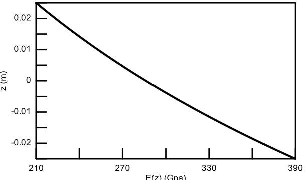
Fig 2 and Fig 3 show both the power and exponential representations of FGM for the variation of the modulus of elasticity along the beam thickness direction. In Fig 2,the power-law, Eq. (3), is drawn for different values of k whereas the FGM beam is assumed to be of E=390 GPa at the lower surface z/h= -0.5, and of E=210 GPa at the upper most surface z/h= 0.5. On the other hand, Fig 3 is drawn for the same material properties using Eq. (5).
Fig 3. Variation of modulus of elasticity along the FGM layer thickness (exponential law).
Based on the first-order shear deformation theory [9], the axial and transverse displacements are given by
0
( , ) ( ) ( )
u x z u x z x (6)
0
( , ) ( )
w x z w x (7)
Where
( )
x
is the angle of rotation of the normal to the mid-surface of the beam,u x
0( )
,w
0( )
x
arethe displacements of the neutral axis in the axial and transverse directions, respectively. The axial, normal and shear strains are given by
0( ) ( ) x
du x d x z
dx dx
(8)
0( )
( )
xz
dw x x
dx
(9)
The constitutive relations for the FGM beam is
( ) 0
0 ( )
x x
xz xz
E z G z
(10)
The principle of virtual displacements implies that the beam equilibrium should satisfy
0.
U V
(11)
Where,
0 L
x x xz xz A
U dAdx
(12)0 0
( ) ( ) L
V q x w x dx
(13)The essential and natural boundary conditions at the fixed (x=0) and free (x=L) ends of the cantilever beam are given respectively as
0
u
(0) = 0,
(0) = 0,w
0(0) = 0 (14)0
Where N, V, and Mare the axial force, shear force and moment, respectively; these values can be expressed in derivative forms of
u x
0( )
,w
0( )
x
and
( )
x
as0
1 2
( ) ( )
du x d x
N c c
dx dx
(16)
0 4 ( ) (x) dw x V c dx (17) 0 2 3 ( ) ( )
du x d x
M c c
dx dx
. (18)
Where, / 2 1 / 2 ( ) h h
c b E z dz
2 / 2/ 2 ( ) h
h
c b zE z dz
/ 2 23 / 2
( ) h
h
c b z E z dz
4 / 2/ 2 ( ) h
h
c b G z dz
(19)Substituting equations (8-12) gives
0 0
/ 2
0 / 2 0 0
( ) ( ) ( ) ( ) ( ) ( ) ( ) ( ) ( ) ( ) L h h
du x d x d u x d x
E z z z
dx dx dx dx
U bdzdx
dw x d w x
G z x x
dx dx
(20)Solving Eq. (20), for
u x
0( )
,
( )
x
and
w0( )x , implies that2 2
0
1 2 2 2
( ) ( )
0
d u x d x
c c
dx dx
(21)
2 2
0 0
2 2 3 2 4
( ) ( ) ( )
( ) 0
d u x d x dw x
c c c x
dx dx dx (22) 2 0 2 ( ) (x) 0.
d w x
d
dx dx
(23)
The assumed solutions for the displacements and the angle of rotation have the following form [3]:
2 0( ) 1 2 3
u x a a x a x (24)
2 3
0( ) 4 5 6 7
w x a a x a x a x (25)
2 8 9 10 ( )x a a x a x
(26)
The solutions, Eqs. (24-26), have a total of 10 constants with six boundary conditions, Eqs. (14-15), with 3 degrees of freedom at each node. Thus, there are only six independent constants, and the other four dependent constants can be written in terms of the six independent ones by substituting equations (24–26) into equations (21–23) and collecting terms to get:
3 2( 5 8),
a a a 1 5 8
7
( )
, 3
a a
a a63a9,a10 1(a5a8).
(27)
After substituting Eq. (27) into Eqs. (24-26), the assumed solutions can be written as
2 0( ) 1 2 2( 5 8)
u x a a x a a x (28)
2 3
0 4 5 3 9 1 5 8
1
( ) ( )
3
w x a a x a x a a x (29)
2 8 9 1 5 8 ( )x a a x (a a x)
. (30)
2 1 1 4 1 3 2
1
/ ( ), 2c c c c c
2
2 2 4 1 3 2 1
/ ( ), 2c c c c c
3 1.
2
(31)
In matrix form Eqs. (28-30) become
0 0
( )
.T
u u w x a (32)
Where,
(33)
The typical finite element used in this paper is assumed to have length L and three degree of freedom at each node, Fig 4. For the left node of the typical element (ith node at x=0) and right node of the typical
element (i+1th node at x = L), Fig 4, using Eqs. (32-33), the following relation can be treated
1ˆ ,
u G a
a G uˆ . (34)Where,
1 (0), (L)
G
ˆ 1 1 1
T
i i i i i i
u u w u w
(35)
By substituting Eqs. (28-30) into (16-18), for the left and right nodes of the typical element the forces and moments can be written in terms of generalized displacements by using Eq. (34) as:
F G
a G
G uˆ K uˆ . (36)Where,
F N(0) V(0) M(0) N L( ) V( )L M( )L
(37)Where
F is the load matrix and
K is the stiffness matrix for the typical element. Non-zero terms of matrices G ,
G and
K are given in the Appendix.Fig 4. Typical finite element used.
For the results of the next section, a Maple code for only four elements with five nodes is written using the above formulation. Thus, the global stiffness matrix is of size 15×15, and the global load matrix is of size 15×1. After introducing the boundary conditions at the fixed support, i.e., at the right hand side of the first element, the size of global stiffness matrix becomes 12×12. However, this code can be extended to higher number of elements to get more accurate results. Furthermore, in the next section two problems will be discussed; one is a verification problem compared with the results presented in
1
2 2
2
2 2
4
3 3 2
1 1 3
5
2 2
1 1 8
9
1 0 0
1 1
( ) 0 0 1 ,
3 3
0 0 0 1
a a
x x x
a
x x x x x a
a
x x x a
a
[3], and in the other one, a more general loading conditions are considered to investigate how FGM selection affect the displacements and stresses in the cantilever beam. However, the above formulation can be slightly modified to treat other beams by modifying the boundary conditions, presented in Eqs. (14-15).
3. Results and Discussions
The first case considered is a verification example; a layered cantilever beam of total length L=500 mm and h=50 mm consists of three layers: upper: steel (E=210GPa, G=80GPa, h=22.5mm), lower: alumina (Al2O3) (E=390GPa, G=137GPa, h=22.5mm), middle: FGM layer (h=5 mm). For this case, a unit
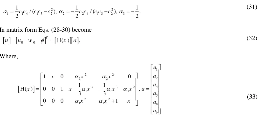
transverse load at the tip is applied; material properties variation considered is exponential, and the beam has a unit width. Figures (5, 6) show the distribution of axial and shear stresses at the fixed point of the beam with and without FGM layer. The result is verified by Chakraborty et al. [3]. In Figures (5, 6),the discontinuity in the stress distributions is noticed due to the mismatch between the layers of two different materials. While the addition of the FGM layer smoothened the curve to about 0.3kPa for axial stress and 0.01kPa for shear stress throughout the thickness.
Fig 5. Axial stress distributions along thickness for transverse load.
Fig 6. Shear-stress distributions along thickness for transverse load.
In the second case, the free end of the beam is assumed to be subjected to axial load, transverse load and a tip-end moment. The geometric properties of layered cantilever beam are taken as L=1000mm, h=50mm and b=50mm. The beam is composed of three layers; the upper layer is made of steel with
E=210GPa and G=80GPa whereas it has a thickness h=10mm. The lower layer is alumina (Al2O3) with
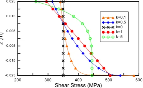
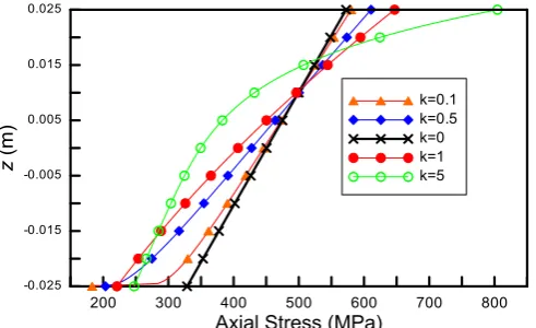
middle layer is considered as FGM with h=30mm. For this case, an axial load of (1000N), transverse load of (1000N) and (1000N.m) moment are applied at the free end. The material properties of the FGM layer obey the power-law, Eqs. (3-4). Figures 7 and 8 show the distribution of axial and shear stresses at the fixed point of the beam for different values of k. From Fig 7, the axial stress distribution for k = 0 is linear, and it is not linear for other values of k. In Fig 8,the shear stress distribution is constant for
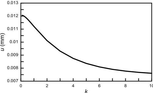
k = 0, and it is linear for k = 1, and then it is varies between them. Figures (9- 11) show the mid plane displacements (axial, transverse, and slope) with different values of k. From Figures (9-11), at low values of exponent k gives higher deflections (axial, transverse, and slope), and the material bending is increased. Figures (12-14) show the maximum points of displacements with the variation of exponent
k. In Figures (12-14), it is obvious that with increasing the exponent k the maximum deflections are decreased which means that the material becomes stiffer in that direction (towards ceramic). For low values of k deflections are higher; the material becomes more elastic (toward metal). Fig 15shows the axial stress distribution along the thickness if the layers considered in drawing Fig 7are reversed upside down. From Fig 15, when the layers of the beam are reversed the most bottom layer becomes metal while the upper is ceramic; at k = 0, the distribution still linear. The stress is higher for lower values of
k (toward ceramic behavior). However, for k=5 the normal stress for at the fixed support becomes smaller when Fig 15 is compared with Fig 7.
Fig 7. Axial stress distributions along beam thickness at different values of k.
Fig 9. Axial deflections along the length at different values of k.
Fig 10. Transverse deflections along the length at different values of k.
Fig 11. Slope along the length at different values of k.
Fig 13. Maximum transverse deflections at different values of k.
Fig 14. Maximum slopes at different values of k.
Fig 15. Axial stress distributions along thickness for reversed layer beam.
4. Conclusions
The results showed that the addition of the FGM layer smoothened the stress distributions along the beam thickness, while there was a stiff jump in the stress distribution in the two-layers beam. The axial and transverse displacements were increased after increasing the amount of load. The variation of Young’s modulus of elasticity due to the power-law has a great effect on stresses and deflections. In the power-law, choosing a suitable value for the exponent k can minimize stresses and deflections to a desired beam condition.
References
[1] Koizumi, M. F. G. M. (1997). FGM activities in Japan. Composites part B: Engineering, 28(2), 1-4.
[2] Chakraborty, A., Mahapatra, D. R., & Gopalakrishnan, S. (2002). Finite element analysis of free vibration and wave propagation in asymmetric composite beams with structural discontinuities. Composite structures, 55(1), 23-36.
[3] Chakraborty, A., Gopalakrishnan, S., & Reddy, J. N. (2003). A new beam finite element for the analysis of functionally graded materials. International journal of mechanical sciences, 45(3), 519-539. [4] García-Vallejo, D., Mikkola, A. M., & Escalona, J. L. (2007). A new locking-free shear deformable
finite element based on absolute nodal coordinates. Nonlinear dynamics, 50(1), 249-264.
[5] Kadoli, R., Akhtar, K., & Ganesan, N. (2008). Static analysis of functionally graded beams using higher order shear deformation theory. Applied mathematical modelling, 32(12), 2509-2525.
[6] Roy, A., & Khan, K. (2013). Static response analysis of a FGM Timoshenko’s Beam subjected to Uniformly Distributed Loading Condition. MIT international journal of mechanical engineering, 3(2), 80–85.
[7] Khan, A. A., Naushad Alam, M., & Wajid, M. (2016). Finite element modelling for static and free vibration response of functionally graded beam. Latin American journal of solids and structures, 13(4), 690-714.
[8] El-Ashmawy, A. M., Kamel, M. A., & Elshafei, M. A. (2016). Thermo-mechanical analysis of axially and transversally Function Graded Beam. Composites part B: Engineering, 102, 134-149.
Appendix:
A.
Non-zero terms of matrix
G :11 21 22
2
2 2
2 1 3 1
2 2
2 3 1 3 1
2 2
2 3 1 3 1
2
3 24 21
25 22 26 32 42 4
2 1 3 1
2 2 2 2
1 3 1 3 1 3 1
3 45 42
46
3 / (3 3)
3 ( 1) / (3 3),
3 /
1, 1 / ,
,
1,
(3 3)
3 / ( (3 3))
(3 3 ) / (3 3),
L L
L L L
L L L
L L L
L L L L
G G L G
G G G
G G G
G G
G G G
G 53 62
63 65 6
2 2
3 1 3 1
2 2
1 1 3 1
2 2 2
1 1 3 1
2 2 2
1 1 3
2
66 1
3 / (3 3),
3 / (3 3)
(2 3) / ( (3 3)),
( 3) / ( (3 3)
1
)
G
G
G G G
G
L L
L L
L L L L
L L L L
B.
Non-zero terms of matrix G :12 16 24 4
25 24 32 16 36 3 42 12 44 1 2 2 1 45 44 46 1
1
6 54 24 55 24 56 3 4 4 62 16 64 1 3 2 2 65 64 66 36
2
, ,
, 2 2
, ,
, 2
, 2 2
,
, ,
G G G c
G G G G G c
G G G L c L c
G G G G G G
G G G L c Lc
G G G L c L c
G G c c G G
C.
Non-zero terms of matrix
K :11 13 14 11 16 13 22
23 25 22 26 23 31 13 32 23
33 34 13 35 36
41 14 43 34 44 46 13 52 2 2
2
1 2 4
4
3 4 23 3 4
11 5 5
1 / (1 / 12)
/ , / L, /
/ 2,
/ ) c / 4, , / ) c / 4
, ,
, , ,
, , ,
( , (
, ,
K K K K K K K
K K K K K K K K K
K K K K K
L
c L c c L
c
c L L K c L L
K K K K K K K K K K K
3 35 55 22
56 23 61 16 62 26 63 36 64 46 65 56 66 33
,
, , , , , ,
K K K
K K K K K K K K K K K K K K