http://www.sciencepublishinggroup.com/j/ijdsa doi: 10.11648/j.ijdsa.20190503.11
ISSN: 2575-1883 (Print); ISSN: 2575-1891 (Online)
Bayesian and Frequentist Approach to Time Series
Forecasting with Application to Kenya’s GDP per Capita
Nathan Musembi, Antony Ngunyi, Anthony Wanjoya, Thomas Mageto
Department of Statistics and Actuarial Science, Jomo Kenyatta University of Agriculture and Technology, Nairobi, Kenya
Email address:
To cite this article:
Nathan Musembi, Antony Ngunyi, Anthony Wanjoya, Thomas Mageto. Bayesian and Frequentist Approach to Time Series Forecasting with Application to Kenya’s GDP per Capita. International Journal of Data Science and Analysis. Vol. 5, No. 2, 2019, pp. 27-41.
doi: 10.11648/j.ijdsa.20190503.11
Received: April 22, 2019; Accepted: May 27, 2019; Published: July 15, 2019
Abstract:
Real GDP per capita is an important indicator of a country’s or regional economic activity and is often used by decision makers in the development of economic policies. Expectations about future GDP per capita can be a primary determinant of investments, employment, wages, profits and stock market activities. This study employed both the frequentist and the Bayesian approaches to Kenya’s GDP per capita time series data for the period between 1980-2017 as obtained from the World Bank data portal. The autoregressive integrated moving average (ARIMA) and the state space models were fitted. The results of the study showed that the local linear trend model and the ARIMA(1,2,1) model are appropriate for forecasting the GDP per capita but the former outperforms the latter. The local linear trend model was used to perform a 3-step ahead forecast and the forecasted value was found to be U.S $ 1717.694, U.S $ 1844.446 and U.S $ 1971.198 for 2018, 2019 and 2020 respectively. The findings of this study showed that the state space models, which utilize the Bayesian approach, outperform the ARIMA models which use the frequentist approach in time series forecasting.Keywords:
ARIMA Model, State Space Model, Kalman Filter, Kalman Smoother, GDP per Capita, Forecast1. Introduction
1.1. Background
Gross domestic product (GDP) is the total value of all the finished goods and services produced within a country’s borders in a specific time period, usually one year [1]. Real GDP per capita on the other hand, is the average income per person in a country or region after isolating the effect of price changes (inflation/deflation). GDP per capita is used by economists to monitor the status and growth of output in an economy and when combined with measures of the purchasing power parity (PPP) it’s used to measure people’s living standard [2]. It has a close correlation with the trend in living standards over time and is used to compare the living standards across countries with different populations. An increase in real GDP per capita of a country means an improvement in the living standards of that country.
Real GDP per capita is a better measure of economic growth because it puts inflation and population change into consideration. As real GDP grows it is assumed that
everyone in the chain will benefit and the growth will have a trickle-down effect on the population, thus improving the standard of living of every person in that economy. A positive or negative change in GDP per capita has a significant effect on the stock market and investors pay attention to this change when coming up with an investment idea or strategy.
and 2017 respectively. Compared to the world’s, Seychelles’ and Luxembourg’s, Kenya’s GDP per capita is far much lower and it’s necessary to formulate policies that aim at its improvement.
Per capita GDP indicates whether an economy is expanding or contracting and can be used as an indication of a nation’s economic growth, decline, or recession. It’s significance as a measure of economic development can be seen in three aspects. Firstly, GDP per capita reflects the level and degree of economic development in industrialized countries. Secondly, is that if individual income levels in a country do not vary much between residents, the data can be used to measure social justice and equality. Finally, GDP per capita has been seen to be related to the level of social stability in a country. Forecasting future economic outcomes is important in the decision-making process in central banks for all countries. Scientific prediction of GDP per capita has important theoretical and practical significance on the formulation of economic development goals.
The ARIMA model, developed by Box and Jenkins, has been one of the most appropriate models for modelling and forecasting future values of a time series data. The study [3] found that the ARIMA (2,2,2) model was the most appropriate model for predicting Kenya’s real GDP, [4] identified the ARIMA (1,1,1) as the best model for predicting the GDP of China and [5] used the Box–Jenkins technique to show that the ARIMA (1,1,0) is the best model for predicting the GDP of Pakistan. However, other empirical studies such as that of the studies [6-7] have shown that there are other models that can outperform the ARIMA models.
According to a study [8] state space model (also known as dynamic linear model) provides a methodology for treating a wide range of problems in time series analysis. In this model, the development of the system over time is determined by an unobserved series of vectors (θ1, θ2,...θn) associated with a series of observations (y1, y2...yn). The application of the Kalman filter in state space modelling leads to Minimum Variance Linear Unbiased Estimates(MVLUE) of the model parameters. State space models can be discussed in three different perspectives; the local level, local level with trend and the basic structural model–more details are found in section 3.3.3. The estimates of future observations of a time series can be made modelled dynamically using the Kalman
filter, while the minimum mean square error
estimators(MMSE) of the model parameters can be computed by a smoothing algorithm [9].
The study [10] compared the forecasts made by a basic form of the structural model with the forecasts made by ARIMA models and concluded that there may be strong arguments in favor of using state space models in practice. In another study [11] showed that a structural time series model is appropriate for analyzing a time series with trend, seasonality, cyclical and a regression component–both in the time and frequency domain. According to a study [12] the posterior probability is spread widely among many models and Bayesian models are superior over choosing any single
model. The study [13] suggested that Bayesian model averaging is a useful alternative to other forecasting procedures especially due to the flexibility by which new information can be incorporated. A study [14] showed that Bayesian models can outperform ARIMA models, especially when forecasting over a short horizon.
An accurate prediction of real GDP per capita is necessary to get an insightful idea of the future trend in living standards. Raw current and historical data cannot be used to develop suitable economic policies and strategies or in the allocation of funds to a particular industry. This requires an accurate, efficient and reliable estimate of GDP per capita for some period ahead. A wide range of models can be used for prediction; each has its own characteristics, advantages and disadvantages. This study aimed at identifying the best statistical model for predicting Kenya’s real GDP per capita. The frequentist (ARIMA model) and the Bayesian (State space model) approaches were used.
1.2. Statement of the Problem
Both real GDP and GDP per capita measure a country’s economic activity but the former is the most widely used measure. However, the latter has a close correlation with the trend in living standards and is a better measure because it puts population growth in to consideration. It is used to compare the standards of living across countries with different populations or from one period to another. The world’s average GDP per capita dropped from U.S$ 10,871.178 in 2014 to U.S$ 10,714.466 in 2017 with Luxembourg recording the highest GDP per capita of US $105,803. In Kenya it rose from U.S$ 1335.123 in 2014 to U.S$ 1,594.834 in 2017 but the living standard in Kenya is still low. A report by KNBS(2018) showed that it’s growth dropped from 2.9% in 2016 to 1.9% in 2017. Accurate prediction is necessary so as to understand the future trend in standards of living. Raw current and historical data cannot be used to develop suitable economic policies and strategies or in the allocation of funds to a particular industry. This requires a reliable estimate of GDP per capita for some period ahead. This study aimed at identifying the best model for predicting Kenya’s real GDP per capita.
1.3. Research Objectives
1.3.1. General Objective
The general objective of this study was to identify the most appropriate model for forecasting Kenya’s real GDP per capita.
1.3.2. Specific Objectives
The specific objectives of the study were:
1.To identify an appropriate state space model for forecasting Kenya’s GDP per capita.
2.To fit an appropriate ARIMA model for forecasting the GDP per capita.
1.4. Significance of the Study
Kenya’s average GDP per capita was U.S $ 1,594.8350 in 2017. This is too low compared to the World’s average GDP per capita of US $10,714.466. Most of the Previous studies on economic growth have put more emphasis on the real GDP rather than the real GDP per capita. A country’s aggregate economic growth is not what matters most; What matters most is whether the people living in a country are getting wealthier. Real GDP per capita puts the aspect of inflation and population growth into consideration making it a good measure of economic growth and indicator of the standards of living. The ARIMA model has been widely used in modelling economic time series data but still there are other models that can be used to model this type of data such as the state space models. One of the advantages of the state space model is that the model parameter estimates are updated as newer information becomes available. This used the most recent data to build statistical models based on the Bayesian and Frequentist approach. The best model was identified and used to perform a 3-step ahead forecast of Kenya’s real GDP per capita.
2. Literature Review
This section presents the theoretical, empirical and conceptual framework. Section 2.1 covers the theoretical literature, section 2.2 is on Empirical literature and section 2.3 presents the conceptual framework. These three sections are further discussed in subsections.
2.1. Theoretical Literature
2.1.1. Classical Theory of Economic Growth
The classical theory of economic growth was developed by Adam Smith, David Ricardo, and Robert Malthus in the eighteenth and nineteenth centuries. The theory states that every economy has a steady state GDP and any deviation off that steady state is temporary and will eventually return [15]. This is because when there is a growth in GDP, population will also increase, leading to a higher demand on the limited resources and the GDP will eventually lower back to the steady state. When GDP goes below the steady state, population will decrease and lead to a lower demand on the resources which in turn will raise the GDP back to its steady state.
2.1.2. Neoclassical Growth Theory
This theory was developed by Robert Solow and Trevor Swan in 1956. According to this theory, economic growth is affected by labor, capital, and technology; but more specifically, technological advances [16]. The output per worker increases with the output per capita but at a decreasing rate, diminishing marginal returns. As per this theory economic growth will not take place unless there are technological advances – which lead to the adjustment of labor and capital. According to this theory, if all nations have access to the same technology, then the standard of living will all become equal. This model fails to explain how technology
is a factor of growth.
2.2. Empirical Literature Review
2.2.1. Forecasting GDP Using the ARIMA Model
The ARIMA methodology has been widely applied by many researchers in modelling and forecasting future GDP rates. The Autoregressive integrated moving average (ARIMA) model was first popularized by a study [17]. The Future values of a time series are predicted as a linear combination of its own past values and a series of random shocks or innovations. ARIMA is an iterative process that involves four stages; identification, estimation, diagnostic checking and forecasting of time series. This model is applied in stationary time series. It can also be applied in non-stationary time series which can be transformed to a stationary time series [18].
The study [3] used Kenya’s GDP time series data for the period between 1960–2012 to build a class of ARIMA models using the Box–Jenkins procedure and showed that the ARIMA (2,2,2) model was the most appropriate model for modelling Kenya’s GDP. [19] used time series GDP data from Shaanxi for the period 1952–2007 to perform a 6–year forecast for the country’s GDP. They identified the ARIMA (1,2,1) model as the most appropriate model for predicting the GDP of Shaanxi.
The study [4] identified the ARIMA (1,1,1) as the best model for fitting the GDP of China using time series data for the period between 1978 to 2006. This was followed by a prediction from 2007 to 2011 and the error between the actual value and the predicted value was small indicating that the ARIMA model is a high precision and effective method to forecast the GDP time series. [20] applied the Box–Jenkins methodology in modelling and forecasting the real GDP rate in Greece using time series data for the period between 1980– 2013. They used the fitted model to forecast GDP for the year 2015, 2016 and 2017. The statistical results showed that Greece’s real GDP rate was steadily improving.
The study [5] used Pakistan’s GDP time series data from 1953 to 2012, which was obtained from the IMF, to construct an ARIMA model for predicting future GDP for Pakistan. After investigating a set of ARIMA models following the Box–Jenkins technique, ARIMA (1,1,0) was found to be the best fit for the data. This model was used for predicting the GDP for Pakistan from 2013 to 2025. The predicted GDP was found to be 23477 Billion and 103918 billion rupees for 2013 and 2025 respectively.
In another study [7] compared the performance of VAR, ARIMA, and Bridge models in forecasting the quarterly GDP growth for Albania. Their empirical results showed that the VAR model outperformed the other models and the ARIMA models portrayed the worst forecast performance compared with the two other models. Again, the ARIMA models performed better than naive models because the Theil’s U Statistic was lower than 1.
2.2.2. Forecasting GDP per Capita
GDP per capita is often used as a measure of economic development and is one of the most important measures in macroeconomics. It is a widely used indicator for country-level income and has been used in modeling health outcomes, mortality trends, cause specific mortality estimation, health system performance and finances, and several other topics of interest. Again, it is one of the most regularly measured economic indicators, with estimates produced quarterly or annually by countries themselves as well as agencies such as the World Bank, UN and the IMF. When combined with the purchasing power parity (PPP), GDP per capita is used to measure people’s standards of living.
The study [21] applied the extrapolation method to estimate the real GDP per capita for more than 100 countries using data for 16 countries. The data for the other countries were estimated using a short-cut method which extrapolates the relationship found for the 16 countries between real GDP per capita and certain independent variables. These estimates were subject to large margin of error but were closer to the true figures than the most commonly used comparisons of nominal GDP per capita.
The study [22] studied the real GDP per capita growth rate of 19 selected OECD member countries for the period between 1950 and 2007. His findings indicated that the growth rate of real GDP per capita is represented as a sum of two components – a monotonically decreasing economic trend and fluctuations related to the change in some specific age population. According to this study, the economic trend is modeled by an inverse function of real GDP per capita with a constant numerator. The Statistical analysis showed that there is a very weak linear trend in the annual increment of GDP per capita for the case of USA, Japan, France, and Italy, and there is a larger positive linear trend in annual increments for the case of UK, Australia and Canada.
In another study [23] investigated the evolution of real GDP per capita in the United States using a two-component model; the first component was the growth trend and the second component was the fluctuations around the growth trend. The trend component was found to be inversely proportional to the attained level of real GDP per capita. The Second component was defined as a half of the growth rate of the number of 9–year–olds. The VAR, VECM, and linear regression were used in estimation of the goodness of fit and RMSE. The highest R2 of 0.95 and the lowermost RMSE was obtained in the VAR representation. The cointegration tests showed that the deviations of real economic growth
from the growth trend are driven by the change in the number of 9–year–olds.
The study [24] considered two methods of forecasting real per capita GDP at various horizons. The univariate time series models estimated country–by–country and the cross–country growth regressions. The results of the study showed that there was only modest differences between these two approaches. Both models performed similarly to forecasts generated by the World Bank’s Unified Survey. The results did not highlight which model outperformed the other but suggested that there are potential gains from combining time series and growth regression-based forecasting approaches.
In summary, there are many models that can be used to forecast macroeconomic time series variables such as real GDP per capita. The study [25] argued that ARIMA models are robust especially when generating short-run GDP forecasts and have frequently outperformed more sophisticated structural models in terms of short-run forecasting ability. Other empirical studies such as that of the studies [6-7] have shown that ARIMA models can be outperformed by other models.
2.2.3. Bayesian Analysis of State Space Models
The Bayesian philosophy was developed by Reverend Thomas Bayes in late 18th century and at this time it was not widely used because of its complexity. Due to its advantages and computational advances, it was revived in the 20th
century and its use in econometrics has increased rapidly since then. In this method, the prior information we possess before seeing the data can be incorporated. The Bayesian paradigm is natural for prediction and takes into account all model parameters and model uncertainty.
The study [11] developed the Bayesian Structural Time Series (BSTS) model which falls under state space models. In this model an unobserved latent state is predicted using noisy measurements of the observed quantity. This model assumes that the noise is normally distributed and that we have some idea of how the latent state evolves over time. The time dependency in this model is computed using a combination of Kalman filtering, Kalman smoothing, and sampling from posterior distributions using Markov Chain Monte Carlo methods.
The study [26] a system for short–term forecasting that averages over different combinations of predictors. The system combined a structural time series model for the target series with regression component capturing the contributions of contemporaneous search query data. Even though their system focused on search engine data to forecast economic time series, they also suggested that the underlying statistical methods could also be applied to more general short-term forecasting with large numbers of contemporaneous predictors.
time-varying volatility and recent approaches to non-parametric Bayesian modelling of time series. They recommend that Bayesian models are alive and well and there is need to explore their advantages.
According to a study [8] state space models provide a methodology for treating a wide range of problems in time series analysis. The development of the system over time is determined by an unobserved series of vectors (θ1, θ2,...θn) associated with a series of observations (y1, y2...yn). The Kalman filtering leads to Minimum Variance Linear Unbiased estimates of the model parameters and can be used to model future observations of a time series. The minimum mean square error estimator of the model parameters can be computed by a smoothing algorithm [9].
The study [10] compared the forecasts made by a structural model with the one made by ARIMA models and concluded that there may be strong arguments in favor of using structural models in practice. In another study [11] showed that a structural time series model is appropriate for analyzing a time series with trend, seasonality, cyclical and a regression component. [12] found that the posterior probability is spread widely among many models and suggested that Bayesian models are superior over choosing any single model.
The study [28] described Practical methods for implementing Bayesian model averaging with factor models. They simulated algorithms that can efficiently select the model with the highest marginal likelihood. The simulated methods were used to forecast the GDP of U.S using data on 162 time series. The results of this simulation indicated that models containing factors outperform autoregressive models in forecasting GDP at short horizons.
2.3. Summary of Reviewed Literature
The reviewed literature focused mostly on ARIMA, state space models, GDP and GDP per capita. Several studies such as that of studies [3, 5, 17, 19-20] showed that the ARIMA model is appropriate for modelling and forecasting GDP. However, other empirical studies such as that of studies [6-7] indicate that the ARIMA models can be outperformed by other models. The study of studies [26-28, 14] have shown that the state space models are the most appropriate models for fitting and forecasting short time series data. Most of the statistical models can be expressed in state space form, including all ARIMA and VARMA models.
2.4. Research Gaps
Most of the past empirical studies identified the ARIMA models as the most appropriate models for fitting and forecasting real GDP or GDP per capita. In these studies, there is little research on real GDP per capita in developing countries with almost none in Kenya. Real GDP per capita responds differently to changes in technology, health and other socio–economic variables. Bayesian models are appropriate for forecasting using time series data, especially over a short horizon, but have been under-utilized because they are
complex. The development of computational algorithms in statistical software has made it easier. [14] recommended that Bayesian models are alive and well and there is need to explore the advantages that can be gained from using Bayesian methods on time series data. This study was meant to bridge this literature gap.
3. Methodology
3.1. Research Design
In this study the experimental research design was used since the data was subject to two different models; with the aim of identifying the best model and then performing a 3-step ahead forecast using the identified model. [29] stated that experimental design is used where there is time priority in a causal relationship, consistency in a causal relationship and where the magnitude of the correlation is great. The longitudinal study design was applied since measurement about our study population was taken sequentially over time at regular time intervals, i.e. annually.
3.2. Target Population, Sampling Frame, Sample Size and Sampling Technique
Target population refers to the the entire group of individuals or objects which the researcher wishes to study and draw conclusions. The target population for this study was Kenya’s GDP per capita. The sampling frame was the real GDP per capita for the period between 1980–2017. If the target population is less than 100, the whole population should be included in the study and a census survey undertaken, (Sperling, Gay, & Airasian, 2003). For this study, a census survey was undertaken since the sampling frame was less than 100, hence no sampling was done. The data used in this study was retrieved from the World Bank’s data portal. The data was available for the time period between 1980 and 2017.
3.3. Data Processing and Analysis
In this study R statistical software package was used to assist in data processing and analysis. The Kenya’s real GDP per capita time series data was used to construct the ARIMA and the state space model. This study focused on the additive time series model which takes the form:
yt = µt + γt+ εt (1)
where ytis the observed value, µtis the trend component, γtthe
seasonality and εtis a random component assumed to be white
noise.
3.3.1. Autoregressive Integrated Moving Average (ARIMA) Model
yt= φ1yt−1 + φ2yt−2 +... + φp yt−p+ εt (2)
while an MA (q) process is expressed as:
yt = ε t − β1ε t−1 − β2ε t−2 −... – βqε t−q (3)
When equation 2 and 3 are combined they yield the ARMA(p,q) process represented by equation 4 below.
yt = φ1yt−1 + φ2yt−2 +... + φp yt−p + εt − β1ε t−1 − β2ε t−2 −... – βqε t−q (4)
A non-stationary ARMA(p,q) process can be transformed to a stationary process through differencing yielding an ARIMA(p,d,q) process as shown below.
Wt = Yt − Yt−1 (5)
= φ1Wt−1 + φ2Wt−2 +... + φpWt−p + εt – β1ε t−1 − β2ε t−2 −... – βqε t−q (6) = φ1(Yt−1 − Yt−2) + φ2(Yt−2 − Yt−3) +... + φp(Yt−p − Yt−p−1)+ εt − β1ε t−1 − β2ε t−2 −... – βqε t−q (7)
Which can be rewritten as:
Yt = (1+φ1)Yt−1 + (φ2 − φ1)Yt−2 + (φ3 − φ2)Yt−3 +... + (φp − φp−1)Yt−p − φpYt−p−1 + εt− β1ε t−1 − β2ε t−2 −... – βqε t−q (8) A time series {Yt} is said to follow an ARIMA model if the
dth difference, Wt = ∆dYt is a stationary ARMA process. The ARIMA (0,0,0) process is known as a white noise process; φi and βj are parameters to be estimated and εt is a white noise process for i = 1, 2,... p, j = 1, 2,..q.
(i). Testing Stationarity
The basic concept of stationarity is that the probability laws that govern the behavior of the process do not change over time. A process {Yt} is said to be strictly stationary if the joint distribution of Yt1, Yt2, Yt3,..., Ytn is the same as the joint distribution of Yt1−k, Yt2−k, Yt3−k,..., Ytn−k for all choices of time points t1, t2, t3,..., tn and all choices of time lag k. If a process is strictly stationary and has finite variance, then the covariance function must depend only on the time lag. A stochastic process {Yt} is said to be weakly stationary if it the mean function is constant over time and cov(yt, yt−k) = cov(y0, yk),
for all time t and lag k ≥ 0.
A time plot for the real GDP per capita gave the general trend of the series. The ADF unit root test was run to determine whether the series was stationary. Since the series was found to be non-stationary, it was transformed to a stationary time series through differencing.
(ii). Box-Jenkins Methodology
Box and Jenkins (1976) developed the ARIMA model for the purpose of forecasting and estimation of a uni-variate time series. In order to use this methodology, one should have either a stationary time series or a time series that can be transformed to a stationary time series. After making the process stationary, the ARIMA(p,d,q) process can be represented by an ARMA(p,q) process as shown in equation (5 & 6) above. If {yt} is an ARMA (p, q) process then:
yt = φ1yt−1 + φ2yt−2 +... + φp yt−p + εt − β1ε t−1 − β2ε t−2 −... – βqε t−q (9)
which can be written as:
yt − φ1yt−1 − φ2yt−2 −... − φp yt−p = εt − β1ε t−1 − β2ε t−2 −... – βqε t−q (10)
where φi and βi are model parameters of the AR and MA parts respectively. Equation (10) above can be re-written as:
Φ(L)Yt = 1 − Θ(L) εt (11)
where:
Φ(yt) = 1 − φ1yt−1 φ2yt−2 −... − φp yt−p (12) Θ(εt) = 1 − β1ε t−1 − β2ε t−2 −... – βqε t−q (13)
(iii). Model Identification
The ACF and PACF plots of the transformed time series was used to identify the order of the AR and MA terms in the ARIMA model. AIC and BIC are given by:
AIC = −2log(L) + 2(p + q) (14)
BIC = −2log(L) + (p + q)log(n) (15)
where: L ≡ the likelihood of the data n ≡ the sample size
p and q ≡ the lag orders of the AR and MA terms respectively.
NB: The model with the lowest AIC or BIC value was be taken to be the best fit for the data.
(iv). Diagnostic Checks
After fitting the model, Diagnostic checking was carried out to ensure that the selected model was the most appropriate. The significance of the model parameters was tested by checking whether the sequence of the residuals formed a white noise process. This was achieved by running the Ljung Box test for independence and the Shapiro-wilks test for normality respectively.
(v). Forecasting Real GDP per Capita
series is to be able to forecast the future values for that series. This study we focused on both the in–sample and out–of– sample forecasting. Based on the available time series data up to time t, i.e., {Yt} = {Y1, Y2, Y3,...Yt−1, Yt}, our aim was to
forecast the value of Yt+mthat will occur m time units into the
future. The minimum mean square error forecast is given by:
Yt(m) = E[Yt+m| Y1, Y2, Y3,...Yt−1, Yt] (16)
3.3.2. Bayes Theorem
A model is recognized as Bayesian when a probability distribution and the Bayes Theorem are used to describe uncertainty regarding the unknown parameters. The Bayesian approach for model formulation begins by first quantifying the researcher’s existing state of knowledge and assumptions [32]. The prior knowledge is then combined with the likelihood function–the joint probability of the data under the stated model assumptions. The posterior distribution is obtained by combining the prior and likelihood information. This combination constitutes the Bayes’ theorem and can be illustrated by the relationship shown below.
posterior ∝ prior × likelihood
Bayes theorem states that the probability that event A occurs, given that event B has occurred, is equal to the probability that both A and B occur, divided by the probability that B occurs: i.e.
| = ∩ (17)
From equation (17) above, if we let A to be a parameter(s) and B the observed data (yt), then we have:
| = ∩ = | × (18)
where:
P (θ|yt) ≡ the Posterior probability.
P (yt|θ) ≡ the likelihood of obtaining the data under the null
hypothesis.
P (θ) ≡ the Prior probability of θ.
P (yt) ≡ the probability of obtaining the data under all
admissible parameter estimates.
3.3.3. State Space/Dynamic Linear Model
The state space models are also known as dynamic linear models (DLM). The idea behind state space models is that an observable yt is generated by an observation or measurement equation, i.e.,
Yt = F’t ′θt + vt (19) where vt ∼ N (0, Vt), and is expressed in terms of an
unobservable state vector θt. θt is modeled dynamically
through a system or transition equation as shown below.
θt = Gtθt−1 + ωt (20)
With ωt ∼ N (0, Wt) and the error terms ωt and vt are
mutually independent. Normality is usually assumed and a prior distribution is required to describe the initial state vector
θ0. The general univariate state space model is represented by equations (19 & 20) where:
Observation Equation: Yt= F’t′θt+ vt, vt∼N (0, Vt),
System Equation: θt= Gtθt−1 + ωt ωt∼N (0, Wt)
Yt≡ the observation series at time t
Ft≡ a vector of known constants
θt≡ the vector of model state parameters
vt≡ a stochastic error term
Gt ≡ a matrix of known coefficients that defines the
systematic evolution of the state vector across time
ωt≡ a stochastic error term having a normal
The two stochastic series {vt} and {ωt} are assumed to be
independent. The dynamic linear model can be broken down further into: Local level model, local linear trend model and basic structural model as follows:
Local level model
Yt = θt + vt, vt ∼ N (0, Vt) (21)
θt = θt−1 + ωt, ωt ∼ N (0, Wt) (22)
Local linear trend model
Yt = θt + vt, vt ∼ N (0, Vt) (23)
θt = θt−1 + βt +ωt, ωt ∼ N (0, Wt) (24)
βt = βt−1 + ηt, ηt ∼ N (0, Ht) (25)
Basic structural model
Yt = θt + γt + vt, vt ∼ N (0, Vt (26)
θt = θt−1 + βt + ωt, ωt ∼ N (0, Wt) (27)
βt = βt−1 + ηt, ηt ∼ N (0, Ht) (28)
s−1
γt = − ∑ γt−j + kt (29)
j=1
(i). The Kalman Filter
The Kalman Filter is a recursive set of equations used to update the estimated parameters as new observations become available. Filtering updated our knowledge of the system each time a new observation ytwas brought in. The idea of updating
in the Kalman Filter is related to the Bayesian approach, indeed the theory behind the Kalman Filter is Bayesian. The Kalman smoothing algorithm was used to obtain the best estimate of the state at any point in the sample. Kalman filtering accumulates information about the time series as it moves forward through the list of the parameters while the Kalman smoother moves backward through time, distributing information about later observations to earlier parameters. Let
yt−1 be the vector of observations (y1, y2..., yt−1)′ for t = 2, 3... and assume that the conditional distributions θt|Yt−1 ∼ N (at,
Pt), θt|Yt∼N (at|t, Pt|t) and θt+1|Yt∼N (at+1, Pt+1) where at and
Ptare known. Our objective is to calculate at|t, Pt|t, at+1 and Pt+1 when ytis brought in. We refer at|tas the filtered estimator of
the state θtand at+1 as the one–step ahead predictor of θt+1. An important part is played by the one-step ahead prediction error
vt = yt − at
According to Durbin and Koopman (2012a), if we let
Zt= V ar(vt|yt−1) and = , then it can be showed that: vt = yt − at, (30)
at|t = at + Ktvt, (31)
at+1 = at + Ktvt, (32)
for t = 1,..., n
= + (33)
Pt|t = Pt 1 − Kt (34)
#$ = 1 − % (35)
The relations showed in the above equation is referred as the Kalman Filter. The Kalman filtering accumulates information about the time series as it moves forward through the list of (at, Pt) elements i.e. mean and variance. The Kalman smoother moves backward through time, distributing information about later observations to successively earlier (at, Pt) pairs.
(ii). Updating Prior to Posterior and Forecasting
Model forecasts were derived from the prior information and the observation equation. The Prior information on the state vector for time (t+1) was summarized as a normal distribution with mean at+1 and covariance Rt+1. θt+1|Dt ∼ N [at+1, Rt+1], where Dt denotes the state of knowledge at time t. From the prior information, forecasts were generated using the observation equation. The forecast quantity Yt+1 is a linear combination of normally distributed variables, θt+1|Dt and vt+1. The forecast mean and variance are given by:
&' #$|( ) = &'*+#$ #$+ ,#$|( ) (36)
= &'*+#$
#$|( ) + &',#$|( )
= *+#$&' #$|( ) + &',#$)
= *+#$-. + 1
= /. + 1
0-1'' #$|( ) = ,-1'*+#$ #$+ ,#$|( ) (37)
= ,-1'*+#$
#$|( ) + ,-1',#$|( )
= *+#$,-1'
#$|( )*+#$+ ,-1',#$)
= *+#$2. + 1 *. + 1
= 3. + 1
The forecast quantity was normally distributed with mean
ft+1 and variance Qt+1. Yt+1|Dt∼ N [ft+1, Qt+1] Given the prior for time (t+1) the implied prior for time (t+2) from the same standpoint, with no additional information is p(θt+2|Dt). This
prior was obtained by applying the system equation as in
θt+2 = Gθt+1 + ωt+2 with ωt+2∼N (0, Wt+2) (38) E[θt+2|Dt] = E[Gθt+1 + ωt+2|Dt]
= E[Gθt+1|Dt] + E[ωt+2|Dt] = GE[Gθt+1|Dt]
= Gat+1
V ar[θt+2|Dt] = V ar[Gθt+1 + ωt+2|Dt] (39) = V ar[Gθt+1 |Dt] + V ar[ωt+2|Dt]
= Gvar[θt+1 |Dt]G′ + Wt+2
= GRt+1G′ + Wt+2
The likelihood, a function of the model parameters, is the conditional forecast distribution evaluated at the observed value and has the normal form given as;
L(θt|Yt = yt, Vt)∝ P(Yt = yt|θt, Vt) ∼ N [Ft ′, Vt] (40)
The prior information is combined with the likelihood to yield the posterior distribution as shown below.
|(4$, = 6 7 | ,8 |9:;
< 6 7 (41)
Forecasting k steps ahead requires the prior information to be projected into the future through repeated application of the system equation.
Yt+k |Dt ∼ N [ft(k), Qt(k)] (42)
4. Results and Discussion
This section presents the results of the fitted ARIMA and state space models that were found to be appropriate models for predicting Kenya’s real GDP per capita. The results of the two models were compared and the best model was used to perform a 3-step ahead forecast of the real GDP per capita.
4.1. Data
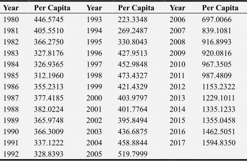
The data used in this study was obtained from the World Bank data portal and organized as shown in the table 1 below.
Table 1. Kenya’s GDP per capita (U.S Dollars) from 1980 to 2017.
Year Per Capita Year Per Capita Year Per Capita
4.2. The ARIMA Model
4.2.1. Trend
A time plot of the observed and smoothed real GDP per capita was fitted so as to get the general trend. The time plot showed an exponentially increasing trend. A plot of Yt against Yt−1 shows that there is a strong correlation between Yt and Yt−1.
Figure 1. Plot of real GDP per capita.
Figure 2. Plot of Yt against Yt-1.
4.2.2. Stationarity of the Data
The Augmented Dickey-Fuller(ADF) test was run at 5% level of significance to check the stationary of the observed and differenced time series. The null hypothesis for this test is that the data was non-stationary. The results of running the ADF test are as shown in table 2 below.
Table 2. ADF test results.
Series P value Dickey Fuller
First difference 0.1025689 -3.2070121
second difference 0.0100000 -4.4660824
The p values obtained on running the ADF test on the observed, first and second difference was found to be 0.99, 0.1025689 and 0.01 respectively. The p-values obtained on the observed and first difference series was greater than the significance level, therefore we failed to reject the and concluded that the first difference and the observed GDP per capita series was non-stationary. However, the p-value obtained by running the ADF test on the second difference was smaller than the level of significance, therefore we rejected the null hypothesis in favor of the alternative hypothesis and concluded that the second difference transformation made the series stationary.
4.2.3. Model Identification
The ACF and PACF plots of the observed and transformed series is as shown in figure 3 below.
Figure 3. ACF and PACF Plots.
The ACF plot of the second difference suggested that the transformed series followed an ARMA(1,1) process. Therefore the appropriate model for fitting the GDP per capita was identified as ARIMA(1,2,1).
4.2.4. Model Fitting
The ARIMA(1,2,1) model identified in the section above takes the form:
Yt = φ1Yt-1 − β1 εt-1 + εt (43)
where φ1 and β1 are parameters to be estimated. These model parameters were estimated through the Maximum likelihood approach and the estimates were found to be:
φ1 = 0.328775 and β1 = −0.8340786
The fitted ARIMA model for the real GDP per capita was identified as:
Yt = 0.328775Yt-1 + 0.8340786εt−1 + εt (44)
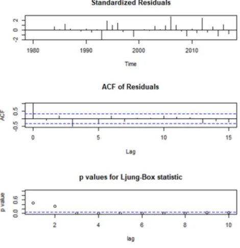
Figure 4. ARIMA diagnostic plot.
4.2.5. Diagnostic Checking
The residuals of the fitted model were examined to check whether they are independent and normally distributed. A plot of the standardized residuals, ACF and P values of the Ljung-Box statistic obtained.
The ACF plot values are within the confidence band except at lag 3 where there is a very weak serial correlation. A plot of the Ljung-Box statistic p values at different lags contains values that are above the significance level indicating that the residuals are independent. Again, the Ljung Box test was run on the standardized residuals of the fitted model to check whether they are independent. The null hypothesis for this test was that the residuals are independent. The p-value obtained from this test was 0.5402776. Based on this p value we failed to reject the null hypothesis and concluded that the residuals were independent. To check whether the residuals were normally distributed, the Shapiro– Wilk test for normality was run and the p-value for this test was 0.1505323. The null hypothesis for this test was that the residuals are normally distributed and based on this p value we failed to reject the null hypothesis; the conclusion was that the residuals were normally distributed. A plot of the residuals, ACF, histogram, density and quantile plot of the residuals is as shown in figure 5.
Figure 5. Diagnostic plots for the ARIMA model.
The plots above together with the Shapiro–Wilk and Ljung box test showed that the residuals of the fitted model are independent and normally distributed. We therefore concluded that the ARIMA (1,2,1) model with φ1 = 0.328775 and β1 = −0.8340786 is a good fit for the real GDP per capita.
4.2.6. Forecasting Real GDP per Capita
A 3-step ahead forecast of the Kenya’s real GDP per capita was performed using the fitted ARIMA (1,2,1) model. The point forecasts at 95% confidence level are as shown in below.
Table 3. ARIMA(1,2,1) forecast.
Year Point Forecast Low 95 High
2018 1696.908 1593.022 1800.793
2019 1789.033 1602.209 1975.856
2020 1877.887 1611.843 2143.930
The in-sample forecast together with the associated 95% confidence interval was found to be:
Table 4. In-sample ARIMA(1,2,1) forecast.
Year Forecast Lower Upper
1980 446.3747 340.36748 552.3820
1981 406.2418 300.23458 512.2491
1982 364.7348 258.72752 470.7420
1983 326.5364 220.52914 432.5437
1984 290.3053 184.29808 396.3126
1985 309.2740 203.26673 415.2813
1986 291.7563 185.74904 397.7636
1987 365.4761 259.46887 471.4834
1988 382.9100 276.90279 488.9173
1989 381.4858 275.47855 487.4931
1990 356.0398 250.03258 462.0471
1991 363.4119 257.40460 469.4191
1992 320.1253 214.11807 426.1326
1993 320.0398 214.03257 426.0471
1994 166.5131 60.50586 272.5204
1995 279.3713 173.36405 385.3786
1996 354.6655 248.65822 460.6727
1997 475.6945 369.68722 581.7017
1998 473.2449 367.23764 579.2522
1999 492.2054 386.19817 598.2127
Year Forecast Lower Upper
2001 398.4311 292.42387 504.4384
2002 401.7965 295.78922 507.8037
2003 393.6598 287.65251 499.6670
2004 457.0138 351.00649 563.0210
2005 473.3930 367.38572 579.4002
2006 554.7406 448.73338 660.7479
2007 793.7878 687.78050 899.7950
2008 931.8674 825.86010 1037.8746
2009 986.0310 880.02374 1092.0383
2010 953.7413 847.73402 1059.7485
2011 1017.7627 911.75539 1123.7699
2012 1023.9464 917.93917 1129.9537
2013 1259.0256 1153.01839 1365.0329
2014 1300.3783 1194.37106 1406.3856
2015 1422.0790 1316.07176 1528.0863
2016 1402.5719 1296.56463 1508.5792
2017 1548.7554 1442.74810 1654.7626
4.3. Fitting the State Space Model
Figure 6. Plot of observed, fitted and predicted values.
4.3.1. Introduction
In this section we focused on two forms of state space models, i.e the local level model (LLM) and the local linear trend model(LLTM). The two models were fitted by use of the Kalman filter and the Kalman smoother. The best state space model was identified and GDP per capita forecasted using this model. The general representation of the state space model is:
Observation Equation:
Yt = F’t′θt + vt, vt∼ N (0, Vt) (45)
System Equation:
θt = Gtθt−1 + ωt ωt ∼ N (0, Wt) (46)
The parameters of this model were obtained by Maximum Likelihood method and the variances were assumed to be
unknown.
4.3.2. Local Level Model (LLM)
A state space model is a local level model if the coefficient of θt and θt-1 in equation is 1. The local level model is represented by the equations:
Observation Equation:
Yt = ′θt + vt, vt∼ N (0, Vt) (47)
System Equation:
θt = θt−1 + ωt ωt ∼ N (0, Wt) (48)
4.3.3. Building the Local Level Model
The local level model was built by setting the order of the model to 1. The maximum likelihood estimates were obtained and the convergence component was zero indicating that the algorithm converged successfully. The estimated model parameters were used to fit a model that was used to generate the filtered and the smoothed estimates with:
Ft = 1, Gt = 1, Vt = 10−4 and Wt = 4840.971764
V and W are the variances of the random components in the observation and transition equations respectively. The BFGS optimization algorithm was used to obtain the maximum likelihood estimates and the optimum estimated hessian matrix. The asymptotic variance matrix of the maximum likelihood estimators is given by the inverse of the Hessian matrix of the negative log likelihood function. The predicted states, filtered estimates of state vectors and smoothed estimates of the state together with the corresponding variances were also obtained.
4.3.4. Diagnostic Checking
The residuals of the fitted model were examined to check whether they are independent and are normally distributed. Several diagnostic plots are shown in figure 7 below.
The Ljung Box test for independence and the Shapiro–Wilk test for normality was performed and the results were as shown in table 5 below.
Table 5. Diagnostic tests for local level model.
Test Statistic P Value
Ljung Box 10.2678065 0.0013537
Shapiro-wilk 0.9619733 0.2199502
The p value obtained upon running the Shapiro–Wilk test was 0.2199502. Based on this p value we failed to reject the null hypothesis and concluded that the residuals were normally distributed. The p value obtained by running the Ljung box tests was 0.0013537. According to this p value we rejected the null hypothesis and concluded that the residuals were not independent but they were correlated. Since the residuals were correlated we concluded that the local level model is not a good fit for the real GDP per capita. What followed is that We considered the Local linear trend model, which is of order 2.
4.3.5. Local Linear Trend Model
A local linear trend model takes the form:
Yt = θt + vt, vt ∼ N (0, Vt) (49)
θt = θt−1 + βt + ωt, ωt∼ N (0, Wt) (50)
βt = βt−1 + ηt, ηt ∼ N (0, Ht) (51)
4.3.6. Building the Local Linear Trend Model
The local linear trend model was fitted using the same steps and functions used to fit the local level model except that the order is set to 2 in the dlmModPoly function and a trend component is added. The maximum likelihood estimates for the parameters were obtained as follows.
Table 6. Local linear trend model Maximum likehood estimates.
V W H Convergence Value
5.535959 -0.1689513 5.535959 0 179.6639
The convergence component was zero indicating that the algorithm converged successfully. The model parameter estimates in equation (49,50 and 51) were identified as:
* = 1 0 , > = ?1 1
0 1@ , 0 = 253.651 -FG H = ?0.844550 2008.15322@0
Where Vt is the observational error variance(V) and Wt is the transitional error variance(W).
4.3.7. Diagnostic Checking
The results obtained upon running the Ljung Box and Shapiro Wilks tests are as follows.
Table 7. Diagnostic tests for local linear trend model.
Test Statistic P value
Ljung Box 0.1337043 0.7146218
Shapiro-wilk 0.9563005 0.1436483
The p value obtained from the Shapiro-Wilk normality test is 0.1436483. We failed to reject the null hypothesis and concluded that the residuals are normally distributed. On the other hand, the p value obtained from the Ljung Box test was 0.7146218. We failed to reject the null hypothesis and concluded that the residuals are independent. The results of the Ljung Box and shapiro Wilk tests showed that the local linear trend model is a good fit for the real GDP per capita.
4.3.8. Forecasting
Both in-sample and out-of-sample forecasting was performed using the fitted local linear trend model. A plot of the observed, fitted(filtered), smoothed and forecasted values is as shown in figure 8 below.
Figure 8. Observed, filtered, smoothed and predicted values.
The 3-step ahead out-of-sample forecast using the local linear trend model is as shown in table 8 below.
Table 8. Out-of-sample filtered forecast.
Year Point Forecast Upper Lower Forecasted state
2018 1717.694 1811.292 1624.096 1717.694 2019 1844.446 2029.791 1659.101 1844.446 2020 1971.198 2269.463 1672.934 1971.198
The in-sample forecast (filtered estimates), smoothed estimates and the associated 95% confidence intervals are as shown in the table 9 below.
Table 9. In-sample forecast of GDP per capita.
Year Filtered Upper limit Lower limit Smoothed Observed
1982 364.5801 462.3291 266.83111 364.9247 366.2750
Year Filtered Upper limit Lower limit Smoothed Observed
1984 289.0982 382.7153 195.48116 321.9435 326.9365
1985 315.1592 408.7593 221.55917 320.3687 312.1960
1986 301.2802 394.8783 207.68212 351.6108 355.2313
1987 382.3445 475.9425 288.74638 375.4391 377.4185
1988 405.2644 498.8625 311.66636 380.3315 382.0224
1989 392.9997 486.5978 299.40165 370.4312 365.9748
1990 355.9658 449.5639 262.36777 363.2887 366.3009
1991 361.5044 455.1024 267.90631 341.1270 337.1222
1992 315.8439 409.4420 222.24585 310.0647 328.8393
1993 314.8671 408.4652 221.26906 244.4151 223.3348
1994 145.4677 239.0658 51.86968 267.3381 269.2487
1995 271.9944 365.5924 178.39630 334.8922 330.8043
1996 384.9532 478.5513 291.35517 418.3584 427.9513
1997 517.2004 610.7985 423.60233 456.5886 452.9848
1998 500.0618 593.6599 406.46374 464.4706 473.4327
1999 496.5946 590.1926 402.99650 428.2758 421.4329
2000 389.2056 482.8037 295.60753 405.3233 403.9797
2001 376.3421 469.9402 282.74405 398.6857 401.7764
2002 393.3335 486.9316 299.73548 400.8021 395.8494
2003 391.1831 484.7812 297.58502 428.6219 436.6875
2004 464.4892 558.0872 370.89111 459.8135 458.8844
2005 486.28 579.8738 392.67770 535.9746 519.7999
2006 570.5270 664.1250 476.92888 691.3676 697.0066
2007 840.0566 933.6547 746.45853 832.0768 839.1081
2008 991.3932 1084.9913 897.79517 908.8995 916.8993
2009 1016.2805 1109.8785 922.68239 928.3006 920.0816
2010 945.4051 1039.0031 851.80700 960.1367 967.3505
2011 1000.7014 1094.2994 907.10329 1009.087 987.4809
2012 1013.1752 1106.7733 919.57717 1137.99 1153.232
2013 1277.2165 1370.8146 1183.6183 1234.805 1229.101
2014 1329.9343 1423.5324 1236.3362 1320.777 1335.1233
2015 1435.8672 1529.4653 1342.2691 1368.2425 1355.0458
2016 1398.8793 1492.4774 1305.2812 1464.1760 1462.5051
2017 1545.1296 1638.7277 1451.53152 1590.9413 1594.8350
4.4. Performance of the Fitted ARIMA and State Space Model
The ARIMA(1,2,1) was identified as the best ARIMA fit for the real GDP per capita while the local linear trend model(LLTM) was identified as the most appropriate state space model. The mean error(ME), standard error(SE), mean absolute error(MAE), mean percentage error (MPE), mean absolute percentage error(MAPE), mean absolute scaled error(MASE), AIC, BIC and the log likelihood were used to compare the accuracy and the performance of the two models. The table below summarizes the performance of the two models.
Table.10. Comparison of the performance of the fitted models.
Metric ARIMA LLTM
SE 8.8339 2.65440
MAE 38.2759 0.74779
MASE 0.7103 0.01094
logLik -194.3463 -179.66393
AIC 380.6926 365.32786
BIC 395.8596 370.24062
The rule of the thumb is that we select the model that maximizes the likelihood, minimizes the errors as well as the AIC and BIC and the one whose R -Squared is closest to one. In this case, the Local linear trend model was identified as the
most appropriate model for fitting and forecasting the real GDP per capita for Kenya.
4.5. Summary of the Forecasts
The predicted values using state space and ARIMA models are as shown in table 11 below.
Table 11. Out-of-sample forecast.
Year ARIMA State space
2018 1696.908 1717.694
2019 1789.033 1844.446
2020 1877.887 1971.198
The Local linear trend model was identified as the best fit and a 3-step ahead forecast of the real GDP per capita is as in table 12 below.
Table 12. Out-of-sample filtered forecast.
Year Point Forecast Upper Lower
2018 1717.694 1811.292 1624.096
2019 1844.446 2029.791 1659.101
2020 1971.198 2269.463 1672.934
Figure 9. Plot of observed, Predicted and smoothed value.
5. Conclusions and Recommendations
5.1. Summary
Expectations about future GDP per capita can be the primary determinant of investments, employment, wages, profits and stock market activities. The ARIMA model uses the frequentist approach in forecasting the future values of a time series while state space models use the Bayesian approach. This study used time series data from the World Bank for the period between 1980-2017 to compare the performance of the ARIMA and state space models. The results of this study showed that the ARIMA(1,2,1) and the local linear trend models are appropriate models for forecasting Kenya’s real GDP per capita. The accuracy of the two models was compared and local linear trend model (a form of state space models) was found to perform better than the ARIMA model because it had a larger log likelihood, minimum MAE, SE, MASE, AIC and BIC and the R -Squared was closer to 1. The findings of this study were found to be consistent with those of [10, 12, 14, 27, 28] who concluded that Bayesian models are alive and well and are appropriate for prediction especially over a short horizon.
5.2. Conclusion
State space models outperform ARIMA models in their forecasting ability. This clearly indicates that the Bayesian approach is superior to the frequentist approach in time series forecasting. The advantage of Bayesian approach is that the model parameters are updated when a new observation is brought in. These models are therefore appropriate for generating future values of a macroeconomic time series.
5.3. Recommendations
The results of this study showed that the state space models which are a class of Bayesian models outperform the autoregressive moving average models which employ the frequentist approach in time series forecasting. We therefore recommend the use of State space models in forecasting the
future values of a macroeconomic time series.
5.4. Suggestions for Further Research
There are many models that can be used to forecast future values of a time series. We suggest further studies to determine whether there are other models that can outperform the state space models in their predictive ability. More research can be conducted to establish ways that can ensure a sustained increase in real GDP per capita especially in developing countries like Kenya.
References
[1] Pavia, M., Jose, M., & Cabrer, B., Borras. (2007). On estimating contemporaneous quarterly regional GDP. Journal of Forecasting, 26 (3), 155–170.
[2] Larsson, H., & Harrtell, E. (2007). Does choice of transition model affect GDP per capita growth?
[3] Musundi, S. W. (2016). Modeling and forecasting Kenyan GDP using autoregressive integrated moving average (arima) models. Science Journal of Applied Mathematics and Statistics, 4 (2), 64–73.
[4] Wang, Z., & Wang, H. (2011). GDP prediction of china based on arima model. Journal of Foreign Economic and Trade, 210 (12).
[5] Zakai, M. (2014). A time series modeling on GDP of pakistan. Journal of Contemporary Issues in Business Research, 3 (4), 200–210.
[6] Hai, V. T., Tsui, A. K., & Zhang, Z. (2013). Measuring asymmetry and persistence in conditional volatility in real output: Evidence from three east Asian tigers using a multivariate garch approach. Applied Economics, 45, 2909– 2914.
[7] Shahini, L., & Haderi, S. (2013). Short term albanian GDP forecast:“one quarter to one year ahead”. European Scientific Journal, ESJ, 9 (34), 198–208.
[8] Durbin, J., & Koopman, S. J. (2012b). Time series analysis by state space methods. Oxford University Press.
[9] Harvey, A. C. (1981). Finite sample prediction and over differencing. Journal of Time Series Analysis, 2 (4), 221–232. [10] Harvey, A. C., & Todd, P. (1983). Forecasting economic time
series with structural and box-jenkins models: A case study. Journal of Business & Economic Statistics, 1 (4), 299–307. [11] Harvey, A. C. (1989). Forecasting, structural time series
analysis, and the kalman filter. Cambridge University Press. [12] Fernandez, C., Ley, E., & Steel, M. F. (2001). Model
uncertainty in cross-country growth regressions. Journal of applied Econometrics, 16 (5), 563–576.
[13] Jacobson, T., & Karlsson, S. (2004). Finding good predictors for inflation: A Bayesian model averaging approach. Journal of Forecasting, 23 (7), 479–496.
[15] Spengler, J. J. (1959). Adam smith’s theory of economic growth: Part i. Southern Economic Journal, 25 (4), 397–415. [16] Solow, R. M. (1956). A contribution to the theory of economic
growth. The quarterly journal of economics, 70 (1), 65–94. [17] Box, G. E., & Jenkins, G. M. (1976). Time series analysis,
control, and forecasting. San Francisco, CA: Holden Day, 3226 (3228), 10.
[18] Hamilton, K. (1994). Green adjustments to GDP. Resources Policy, 20 (3), 155–168.
[19] Wei, N., Bian, K., Yuan, Z., et al. (2010). Analysis and forecast of shaanxi GDP based on the arima model. Asian Agricultural Research, 2 (1), 34–41.
[20] Dritsaki, C. (2015). Forecasting real GDP rate through econometric models: An empirical study from greece. Journal of International Business and Economics, 3 (1), 13–19. [21] Kravis, A. W., Irving B Heston, & Summers, R. (1978). Real
GDP per capita for more than one hundred countries. The Economic Journal, 88 (350), 215–242.
[22] Kitov, O. I. (2009). The evolution of real GDP per capita in developed countries. Journal of Applied Economic Sciences, 4 (2), 221–234.
[23] Kitov, I. O., Dolinskaya, S. et al. (2009). Modelling real GDP per capita in the (usa): Cointegration tests. Journal of Applied Economic Sciences, Spiru Haret University, Faculty of Financial Management and Accounting Craiova, 4 (1), 7.
[24] Kraay, A., & Monokroussos, G. (1999). Growth forecasts using time series and growth models. The World Bank.
[25] Stockton, D. J., & Glassman, J. E. (1987). An evaluation of the forecast performance of alternative models of inflation. The Review of Economics and Statistics, 69 (1), 108–117. [26] Scott, S. L., & Varian, H. R. (2013). Predicting the present with
Bayesian structural time series. Available at SSRN 2304426. [27] Steel, M. F. J. (2010). Bayesian time series analysis. In S. N.
Durlauf & L. E. Blume (Eds.), Macroeconometrics and Time Series Analysis (pp. 35–45). London: Palgrave Macmillan UK. [28] Koop, G. M., & Potter, S. (2003). Forecasting in Large Macroeconomic Panels Using Bayesian Model Averaging. SSRN Electronic Journal.
[29] Leedy, P. (1997). Practical research: Planning and design. New Jersey: Prentice-Hall.
[30] Kothari, C. R. (2004). Research methodology: Methods and techniques. New Age International.
[31] Sperling, R. A., Gay, L., & Airasian, P. W. (2003). Student study guide to accompany lr gay and peter airasian’s educational research: Competencies for analysis and application. Merrill.