ISSN: 2334-2382 (Print), 2334-2390 (Online) Copyright © The Author(s). 2014. All Rights Reserved. Published by American Research Institute for Policy Development
Does Microcredit Reduce Household Vulnerability to Poverty? Empirical Evidence from Bangladesh
Khan Jahirul Islam1
Abstract
Household poverty is a dynamic phenomenon, and thus requires dynamic analyses rather than traditional static measurements. We argue that if we use dynamic measurements of poverty, microcredit does not reduce a household’s poverty. Not only that, it may increase vulnerability to poverty for chronically poor households. These results contradict most of the existing literature that measures poverty with static methods. We analyzed our data both with static and dynamic measurements, and find the same results as the existing literature when using static measures. Thus, we argue that impact analyses of micro-credit need to incorporate the dynamic nature of poverty.
Keywords: Micro-credit; vulnerability to poverty; dynamics of poverty; FGLS
The availability of credit is important for the lives of poor rural households in the developing world. However, these households are mostly excluded from the formal banking system because they lack capital assets for collateral, and have low income levels. Micro-credit programs offer small loans to the poor to undertake projects that generate income to support themselves and their families; most of these
loans do not require collateral. 2 The system has become a favourite of anti-poverty
schemes, due in large part to its track record in the last 30 years helping the poor in countries such as Bangladesh or India.
The popularity of micro-credit programs is evident in many developing countries. In Bangladesh alone, it effectively covers some 18.1 million households without overlapping, with 62 percent of them are living below the poverty line (Microcredit Regulatory Authority, 2006).
1 PhD candidate, Department of Economics, University of Manitoba, Winnipeg, Manitoba, R3T 5V5
Canada. E-mail: kjahirul_islam@hotmail.com
Academics are still debating the actual effect of micro-credit in improving the wellbeing of the poor (Montgomery and Weiss, 2005). The literature shows that micro-credit programs have either a positive or limited impact on poverty reduction (Hulme & Mosley, 1996; Zeller & Meyer, 2003; Amin, Rai, & Topa, 2001). Nevertheless, these studies measure poverty the traditional way by looking at household observed expenditures or consumption levels, which tells us little about their future poverty prospects. Given the dynamic nature of poverty, there is a need to analyze the impact of micro-credit programs on the vulnerability to poverty of the poor. Access to micro-credit programs is supposed to help the poor through two channels that are related to a household’s vulnerability to poverty: income generation and consumption smoothing (Chaudhuri, Jalan, & Suryahadi, 2002). This paper proposes to assess the impact of access to micro-credit programs on a household’s vulnerability to poverty through a dynamic analysis of poverty.
The objective of this study is to answer the following questions: i) Does access to micro-credit programs reduce a household’s vulnerability to poverty? ii) Does this effect differ among groups of vulnerable households with different characteristics?
This paper is divided into five sections. In Section I, we give an over-review of the empirical and theoretical literature that analyzes the effect of micro-credit on poverty. In Section II, we describe the sample data used in the empirical analysis of this study. In Section III, we present the empirical models that use dynamic measurements of poverty. In Section IV, we discuss our results, and compare the dynamic model and the static models. Finally, we conclude by outlining suggestions for future research.
I. Literature Review
Therefore, the traditional static approaches to measure poverty fail to capture such dynamic properties.
Various studies suggest that a dynamic approach should be used in measuring households’ vulnerability to poverty (Chaudhuri, Jalan, & Suryahadi, 2002; Amin, Rai, & Topa, 2001). Vulnerability to poverty measures the ex ante poverty; that is, it measures who is likely to be poor and how poor they are likely to be. By definition, vulnerability assessment is forward-looking. This is particularly important for policies that are designed to have long-term effects on poverty reduction, which currently rely on a temporal measurements of poverty. Although ideally we would use panel data to estimate vulnerability at the household level, Chaudhuri et al. (2002) argue that we can achieve the same through analysis using cross-sectional data by careful selection of variables. The validity of this method stems from how differences in vulnerability to poverty among households can be attributed to variations of certain household characteristics, such as gender, age, education and main occupations of the household heads. In their proposed method, vulnerability to poverty is measured as the probability that a household’s expected consumption will fall below a predetermined level.
The merits of micro-credit programs are thought to be channeled either through consumption-smoothing mechanisms and/or income generating production. In either case, having access to micro-credit programs should improve a borrowing household’s ability to cope with potential shocks, thus reduc its vulnerability to poverty (Morduch, 1999).
II. Data
One should ideally use panel data of sufficient length and richness to estimate vulnerability at the household level. However, such datasets are rare, especially for poor developing economies. Instead, we can use cross-sectional household surveys with detailed data on household characteristics such as consumption expenditures and income (Chaudhuri, Jalan, & Suryahadi, 2002). This study uses data collected from rural northern Bangladesh using the “Structured Personal Interview” method. The data is collected through stratified random sampling. The dataset includes information on rural households’ socio-economic conditions, such as income and expenditure, credit, education, land and asset holdings, as well as other community characteristics.
The data was collected from three villages in northern Bangladesh along the
Surma basin.3 The villages were chosen for the intensity of poverty and availability of
the both borrower and non-borrower households. The majority of households generated income from agriculture and related activities. The researchers collected data from two types of households, borrowers and non-borrowers of micro-credit. The measurement unit of the target population was the household and 110 were surveyed. Out of those, more than 60 percent were borrowing from one or more micro-credit institutions. (Table 1) All of the borrower households have been borrowing for a minimum of one year and more than 80 percent have been borrowing for more than three years. The detail household characteristics are in Table 1 of Appendix.
Table1. Distribution of Household by Borrowing Status
Category Total
Microcredit Borrower 70
Microcredit Non-Borrower 40
Total 110
3 These three villages are: Enat Nogor, Khadirpur and Islampur. They are part of the South
III. Methodology
Our analysis consists of the following steps: estimating expected consumption, evaluating vulnerability to poverty for each household, examining the relationship between access to micro-credit programs and household vulnerability to poverty, and finally comparison of the impact of access to microcredit programs on poverty reduction between dynamic and traditional static method. In order to measure vulnerability, we use the methods developed by Chaudhuri et al (2002), where a household’s vulnerability level at time t is the probability of its expected consumption level to remain below the poverty line at time t+1. To assess the impact of a micro-credit loan on household vulnerability to poverty, we regress the estimated vulnerability of individual household on a set of household characteristics. One of our main interests is to examine the dummy variable for access to micro-credit, and see if it has a significant effect on vulnerability to poverty.
i) Estimation of Household’s Vulnerability to Poverty Using Expected Consumption
We define vulnerability as the expected poverty in the near future conditioned
on a household’s current characteristics. For a given household h, its vulnerability Vh
at time t is the probability of the log of its expected consumption ̂ to be below
the log of the poverty line ̅ at time t+1:
= ( ̂ < ̅) (1)
In order to compare the expected consumption and the poverty line, we first estimated expected household consumption using a set of household characteristics
in the following form:
= + 2)
where stands for per capita consumption expenditure for household h; Xh
represents a set of observable household characteristics; β is a vector of parameters,
and εh is a mean-zero disturbance term. Consumption expenditure is assumed to be
log normally distributed, as is the disturbance term h. We also assume that the
variance of log consumption varies with the values of household characteristics, .
In order to obtain an efficient estimate of , and following Chaudhuri, Jalan and Suryahai (2002), we use the feasible generalized least square (FGLS) method to
achieve a homoscedastic variance . First, we saved the OLS estimated residual
from equation (2) and used its square to estimate the following using another OLS procedure:
̂ = + (3)
Then we use the fitted value to transform equation (3) as follows:
,
= Γ+ (4)
The above transformed equation is estimated using OLS to obtain an asymptotically
efficient estimate of standard error , which is expressed as:
= Γ (5)
The set of household characteristics, used in the estimation of equation
(2) includes the age, gender, and years of education of the household head, the size of the household, a dummy variable for the main occupation of the head of the household, dependency ratio, the size of the owned and leased land, and a dummy variable for ownership of income generating assets. Based on current literature, elderly male-headed households with higher levels of education are expected to have higher incomes; hence these households will have higher expected consumption levels. In a rural economy, such as Bangladesh, the bulk of a household’s income comes from the main occupation of the household head. The dummy for the main occupation of the household-head takes on a value of one if the head works in agriculture and related industries, and zero otherwise. The dummy for ownership of income generating assets is equal to one if the household owns any, and zero otherwise.
The dependency ratio is defined as the ratio of the number of dependents to the size of the household. A higher dependency ratio is expected to lower a household’s consumption level by reducing their average consumption. In addition, we expect that the age of the household head, size of the household, and land holding (both leased and owned land) will have a non-linear relationship with consumption. Therefore, the model includes the squared terms of these variables.
In order to estimate a household’s vulnerability to poverty , we used the
fitted value of log consumption ln ̂h and the efficient estimation of the standard error
of the consumption function to transform equation (1) in the following way:
= (ln ̂h < ln ̅| Xh) =Φ
̅
. (6)
The poverty line ̅ is calculated based on the Cost-of-Basic-Needs (CBN)
approach. According to the CBN method, a household is defined as poor if its per
capita consumption expenditure lies below a certain level.4 The per capita
expenditure of a household is the amount of money needed to buy an exogenous set
of low-cost adequate food and other requirements. The function Φ ̅ denotes
the cumulative density function of the standard normal distribution of the log consumption.
ii) Categorizing Households
Following Suryahadi and Sumarto (2003), we categorized the sample
households into several groups based on their current consumption , estimated
expected consumption ̂ , and estimated vulnerability level .
(Table 2) Given that vulnerability to poverty is a probability, we use 0.5 as the vulnerability threshold. The existing literature supports this choice of threshold because it is where the expected log consumption coincides with the log of the poverty line (Chaudhuri, Jalan, & Suryahadi, 2002; Suryahadi & Sumarto, 2003).
It is also reasonable to assume that a household is more vulnerable if it has a 50 percent or higher chance of falling into poverty in the near future.
Table 2. Categorization of Households Current Consumption
< ̅* ≥ ̅*
V u ln e rab ili ty t o P o v e rt
y ≥ 0.5 A B ̂ < ̅
E st im at e d E xp e c te d C o n su m p tio n
< 0.5 C D ̂ ≥ ̅
Poor = A + C
Chronic Poor = A
Transient Poor = C
Non-poor = B + D
High Vulnerability Non-poor = B
Low Vulnerability Non-poor = D
High Vulnerability Group = A + B Low Vulnerability Group = D
Total Vulnerable Group = A + B +C
A total of five groups of households emerge: the “poor”, the “non-poor”, the “high vulnerability group”, the “low vulnerability group”, and the “total vulnerable group”. Based on current consumption levels, the population is divided into the “poor” and the “non-poor” groups. Those households whose current consumptions are equal to or below the poverty line are the “poor”; the rest are “non-poor”. The poor households are composed of two distinct groups: the “chronic poor” and the “transient poor”. The chronic poor are households who are currently poor, have expected consumption level below the poverty line, and whose estimated vulnerability is higher than the threshold. These households are most likely to remain poor in the near future.
The “high vulnerability non-poor” are those household whose current consumption is greater than the poverty line but whose expected consumption is lower than the poverty line, and whose vulnerability level is above the threshold.
For the purpose of this study, we focus the analysis on the “high vulnerability” group, which consists of both the chronic poor and high vulnerability non-poor. We also examined the “total vulnerable” group, which is the combination of both the “high vulnerability” group and the transient poor.
iii) Evaluating the Impact of Micro-credit Programs on Vulnerability to Poverty
In order to study the determinants of vulnerability to poverty, we considered the following equation using the 2-stage least square method:
= + (7)
where is the estimated vulnerability to poverty from equation (6); Z is a
combination of household characteristics used in equation (2) plus a dummy of access to micro-credit programs, which takes the value of one if the household is a borrower
and zero otherwise; is a vector of coefficients, and is the error term. The
estimations are performed for two groups of the sample households, the “high vulnerability” group and the “total vulnerable” group.
In this model, the variable “access to micro-credit” is assumed to be correlated with some household’s characteristics that are not included in our model. In order to solve the endogeneity problem, we used the dependency ratio as an instrumental variable (IV). The theoretical justification for using dependency ratio is that a household with more dependents is more likely to borrow microcredit due to financial needs. We used a Probit regression to determine the relationship between the dependency ratio and access to micro-credit. We found that the dependency ratio is not statistically significantly related with vulnerability to poverty but it significantly determines if a household is a borrower of micro-credit.
iv) Static and Dynamic Approach
=Κ + (8)
= 1
0 −
where K is some combination of household characteristics5 plus a dummy
variable for access to micro-credit, as in equation (7). A household is defined as poor if its current consumption levels lie below the poverty line, and as non-poor otherwise. Because the dependent variable is a dummy, an IV-Probit model is used to estimate equation (8). The dependency ratio is used as the IV in this case as well. The purpose for this comparison is to demonstrate how the impact of access to micro-credit on poverty reduction differs depending on how one measures poverty.
IV. Results and Discussion
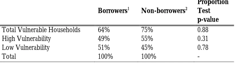
Based on the grouping scheme of households illustrated in the previous section, we found that 70 out of 110 households took micro-credit loans. About half of the borrowers are “high vulnerability” households, and more than half of the 40 non-borrowers are highly vulnerable. Non-borrowers have a larger proportion of households belonging to the “total vulnerable” and “high vulnerability” groups; however we found the proportion differences between borrowers and non-borrowers to be statistically insignificant after using the Proportion test. (Table 3) This indicates that the proportional differences between borrowers and non-borrowers may stem from differences in sample size, and is not due to differences in household characteristics.
5 excludes these variables from : gender of the household head, and income generating asset
Table 3: Summary Statistics of the Categorization of Households and Proportion test
Borrowers1 Non-borrowers2
Proportion Test p-value
Total Vulnerable Households 64% 75% 0.88
High Vulnerability 49% 55% 0.31
Low Vulnerability 51% 45% 0.78
Total 100% 100% -
1.
In total, 70 household are borrowers of micro-credit.
2. In total, 40 households are non-borrower of micro-credit.
Based on the regression using a dynamic measurement of poverty, we found that being a borrower of micro-credit does not increase a household’s vulnerability to poverty for the “total vulnerable” group. The coefficient estimation of the borrower dummy variable is positive, but statistically insignificant. Meanwhile, age, gender, years of schooling and main occupation of the household head are significant determinants of a household’s vulnerability to poverty. A household’s vulnerability to poverty is lower if the head is an elderly male. With increasing years of education of the head of the household, the household’s vulnerability to poverty decreases. The size of leased land and ownership of income generating assets are also positively related to reduction of a household’s vulnerability to poverty. We did not find land ownership to be a determinant of vulnerability to poverty since the majority of households in our sample own limited amounts of cultivable land and cannot reach a profitable production scale. Azam and Imai (2009) found that chronic poverty is widespread among households whose main income relies on agricultural production. Our findings support this claim; if the head of a household works in agriculture and related industries, the household will be more vulnerable to poverty than if their main income came from non-agricultural activities. The regression results for this group are presented in Table 2 of the Appendix.
We found that being a borrower of micro-credit significantly reduces a household’s poverty level, as measured by their current consumption. In fact, taking a micro-credit loan is the most deterministic factor in reducing poverty. In their survey of empirical studies on the effectiveness of micro-credit, Montgomery and Weiss (2005) found that micro-credit almost always has a positive poverty reduction effect on poor households if one measures poverty using current consumption. The static model regression results for the “total vulnerable” group are in the Table 3 of the Appendix.
We found that borrowing micro-credit will increase vulnerability to poverty for the “high vulnerability” group, and this relationship is statistically significant. This result is noteworthy, especially given that the static model shows that for this group of households, taking micro-credit loans should reduce their poverty levels significantly. For the “high vulnerability” group, we found that a female headed household will have lower vulnerability to poverty than a male-headed household. Other determinants of vulnerability are found to have a similar relationship as the findings for the “total vulnerable” group. The dynamic and static model regression results for this group of households are presented in the Table 4 and 5 of the Appendix.
The differences in household characteristics between the two focus groups may explain why micro-credit increases the vulnerability for one group while it has no effect on the other. Within the “total vulnerable” group, we found that a large proportion of households are transiently poor. These households are on their way to escape poverty. Although their current consumption levels are below the poverty line, their predictable consumption in the near future is going to be above it, and thus have lower vulnerability to poverty. On the contrary, within the highly vulnerable group, there are relatively larger proportions of households who are chronically poor. These households are likely to remain in poverty in the future, due to their low consumption levels now and in the near future. Subsequently, if these chronically poor households choose to take micro-credit loans, their priorities will be to increase spending on consumption to meet their basic needs. As a result, it is unlikely that they will invest in income generating production activities, especially given that the size of the credit is usually small. Hence, this group of households will be more vulnerable to poverty.
Within our sample of 70 borrower households, 44 percent of them reported that they borrowed to increase current consumption and only 33 percent indicated that the purpose of borrowing is to use the loan to generate additional income. Furthermore, only 16 percent of the borrower households were able to generate new self-employment through micro-credit. Researchers have shown that the success of NGO-led micro credit programs depends critically on monitoring how loans are allocated. Without monitoring, poor households do not always have the knowledge or skills to improve their wellbeing by making the right investment choices. However, we found that within our sample, 75 percent of borrowers had no guidance from the issuing agencies.
V. Conclusion
Although arguably a helpful and important mechanism in the fight against chronic poverty, micro-credit falls short from being a miraculous cure. In this study we found that having access to micro-credit leads to an increase in vulnerability to poverty, especially for the groups of households that consisted of the more chronically poor. Poverty is a complex issue, and it is crucial to measure it appropriately when evaluating the effectiveness of micro-credit. As we have demonstrated, static measurements of poverty based on current consumption expenditures can lead to deceptive results. These measurements do not incorporate a household’s future state of poverty, and therefore fail to fully evaluate how effective micro-credit programs are in reducing poverty. Our findings show that we do not have the evidence to convincingly argue that micro-credit contributes to reductions in poverty.
Bibliography
Amin, S., Rai, A. S., & Topa, G. (2001). Does Microcredit Reach the Poor and Vulnerable? Evidence from Northern Bangladesh. CID Working Paper NO.28, Center for International Development at Harvard University.
Azam, M. S., & Imai, K. S. (2009). Vulnerability and Poverty in Bangladesh. ASARC Working Papers, Australian National University, Australia South Asia Research Centre.
Chaudhuri, S., Jalan, J., & Suryahadi, A. (2002). Assessing Household Vulnerability to Poverty from Cross-Sectional Data: A Methodology and Estimates from Indonesia. Discussion Paper #0102-52, Columbia University, Department of Economics . Hulme, D., & Mosley, P. (1996). Finance Against Poverty (Vol. 1 and 2). London: Routledge. Kamanou, G., & Morduch, J. (2005). Measuring Vulnerability to Poverty. In S. Dercon (Ed.),
Microcredit Regulatory Authority. (2006, June). NGO-MFIs in Bangladesh. Retrieved April 9th, 2011, from Bangladesh Bank:
http://www.bangladesh-bank.org/pub/annual/mrru/ngomfisbd.html
Montgomery, H., & Weiss, J. (2005). Great Expectations: Microfinance and Poverty Reduction in Asia and Latin America. ADB Institute. ADB Institute.
Morduch, J. (1999). The Microfiance Promise. Journal of Economic Literature , XXXVII, 1569-1614.
Suryahadi, A., & Sumarto, S. (2003). Measuring Vulnerability to Poverty in Indoesia Before and After the Economic Crisis. Asian Economic Journal , 17 (1), 45-64.
Zaman, H. (1999). Accessing the Poverty and Vulnerability Impact of Micrto-Credit in Bangladesh: A case study of BRAC. The World Bank, The Chief Economist and Senior Vice-President (DECVP) .
Zeller, M., & Meyer, R. L. (Eds.). (2003). The Triangle of Microfiance: Financial Sustainability, Outreach and Impact . Johns Hopkins University Press . Appendix
Table 1. Summary Statistics for Explanatory Variables
Variables Mean Stander
Deviation
Household per capita expenditure 12120.6 4148.1
Age of the household-head 40.1 11.9
Household size 6.0 2.2
Education of the household-head (years of
schooling) 0.8 1.4
Dependency Ratio 0.8 0.1
Leased Land 2.6 7.4
Owned cultivable land 1.4 4.0
Variables Category Frequency Percentag
e
Dummy, Income Generating Asset Yes 54.0 49.1
NO 56.0 50.9
Dummy, Main occupation of the
household-head Agricultural 78.0 70.9
Non-Agricultural 32.0 29.1 Dummy, Gender of the household-head Male 96.0 87.3
Table 2. Regression Result for Determinants of Vulnerability, the Total Vulnerable Group
Number of obsservation=75 Wald chi2(13) = 616.53 Prob > chi2=0.00 R-squared=0.885 Root MSE=0.095
Vulnerability Coef. Std. Err. Z P>|z|
Dummy, Borrower 0.138 0.110 1.250 0.210
Age of Head of Household -0.100 0.007 -14.870 0.000
Age2 0.001 0.000 12.830 0.000
Gender of Head of Household 0.121 0.047 2.600 0.009
Household Size 0.060 0.032 1.850 0.065
Household Size2 0.003 0.002 1.100 0.271
Years of education of Head of Household -0.091 0.011 -8.610 0.000 Main Occupation of Head of Household -0.345 0.027 -12.630 0.000
Leased land 0.037 0.008 4.900 0.000
Leasedland2 -0.001 0.000 -5.420 0.000
Owned Cultivable land 0.022 0.019 1.200 0.229
Owned Cultivable land2 -0.001 0.001 -1.170 0.240
Dummy, Income Generating Assets 0.146 0.029 5.100 0.000
Constant 2.331 0.145 16.080 0.000
Table 3. Static Model, the Total Vulnerable Group Number of Observations=68
Wld Chi2(11) =94.42 Prob>chi2=0.00 Log likelihood=-48.56
Poverty Coef. Std. Err. z P>|z|
Dummy, Borrower -2.406 0.256 -9.410 0.000
Age of Head of Household 0.151 0.095 1.590 0.112
Age2 -0.002 0.001 -1.640 0.100
Household Size -0.621 0.629 -0.990 0.323
Household Size2 0.060 0.053 1.130 0.258
Years of education of Head of Household 0.147 0.125 1.180 0.240 Main Occupation of Head of Household 0.251 0.348 0.720 0.471
Leased land -0.158 0.079 -1.990 0.046
Leasedland2 0.006 0.004 1.550 0.121
Owned Cultivable land -0.411 0.153 -2.690 0.007
Owned Cultivable land2 0.023 0.014 1.680 0.094
Table 4. Regression Result for Determinants of Vulnerability, the High Vulnerability group
Number of observations =55 Wald chi2(13) =628.54 Prob > chi2 = 0.00 R-squared = 0.92 Root MSE = 0.04
Vulnerability Coef. Std. Err. z P>|z|
Dummy, Borrower 0.080 0.039 2.040 0.042
Age of Head of Household -0.106 0.006 -18.740 0.000
Age2 0.001 0.000 18.010 0.000
Gender of Head of Household -0.044 0.033 -1.340 0.180
Household Size 0.150 0.025 6.010 0.000
Household Size2 -0.003 0.002 -1.620 0.105
Years of education of Head of Household -0.099 0.007 -14.860 0.000 Main Occupation of Head of Household -0.347 0.021 -16.340 0.000
Leased land 0.031 0.005 6.820 0.000
Leasedland2 -0.001 0.000 -6.180 0.000
Owned Cultivable land 0.016 0.008 2.040 0.042
Owned Cultivable land2 -0.001 0.001 -1.400 0.162
Dummy, Income Generating Assets 0.104 0.019 5.570 0.000
Constant 2.409 0.117 20.510 0.000
Table 5. Static Model, the High Vulnerability group Number of observation= 55
Wald chi2(11) =37.79 Prob > chi2 =0.0001
Log likelihood = -37.793001
Poverty Coef. Std. Err. z P>|z|
Dummy, Borrower -2.335 0.522 -4.480 0.000 -3.358
Age of Head of Household 0.117 0.146 0.800 0.423 -0.169
Age2 -0.001 0.002 -0.650 0.513 -0.004
Household Size 0.020 1.088 0.020 0.985 -2.112
Household Size2 0.034 0.092 0.380 0.707 -0.145
Years of education of Head of Household 0.265 0.238 1.120 0.265 -0.201 Main Occupation of Head of Household 0.065 0.498 0.130 0.897 -0.912
Leased land -0.190 0.172 -1.110 0.269 -0.527
Leasedland2 0.007 0.010 0.740 0.459 -0.012
Owned Cultivable land -0.316 0.281 -1.120 0.261 -0.866 Owned Cultivable land2 0.007 0.026 0.250 0.799 -0.044