Forestry & Natural-Resource Sciences Last Correction: Mar. 8, 2013
SELF-THINNING LIMITS IN TWO AND THREE DIMENSIONS
Oscar Garc´
ıa
Professor, University of Northern British Columbia, Prince George, BC, Canada
Abstract.The principles behind self-thinning laws and stand density management diagrams are exam-ined. Relationships are analyzed based on trajectories of unthinned and thinned stands in a 3-dimensional state space. Limiting self-thinning lines and planes are demonstrated using a dynamic stand growth model for loblolly pine.
Keywords: Forest growth and yield; Reineke; 3/2 law; Relative spacing; Stand density manage-ment diagrams; Thinning; Loblolly pine
1
Introduction
Self-thinning “laws” or rules are a popular topic in forestry. They correspond to limiting straight lines when plotting trees per unit areavs.certain stand variables in logarithmic coordinates (Burkhart and Tom´e 2012, Sec-tion 8.2). Although these relaSec-tionships are based on em-pirical observation and have no satisfactory theoretical basis, conformance to their predictions has been pro-posed as a test of biological realism for growth mod-els (Leary 1997, Monserud et al. 2005, Weiskittel et al. 2011, Section 15.2.3). Even models claiming to be based on physiological processes may rely on them for mod-elling mortality (e. g. Landsberg and Waring 1997). The rules are also behind stand density management dia-grams (SDMDs Drew and Flewelling 1979, Jack and Long 1996).
We examine some of the principles involved, using the LobDyn growth model (Garc´ıa et al. 2011) for illustra-tion. The following section presents the most common self-thinning rules and shows to what extent the be-havior of LobDyn, which was developed independently of such assumptions, agrees with them. Section 3 dis-cusses SDMDs, their uses and limitations. Self-thinning rules and SDMDs are interpreted in Section 4 through projections of 3-dimensional trajectories. This view ex-plains how the various rules are related, and the capa-bilities of SDMDs for projecting growth of thinned and unthinned stands. Limiting 3-dimensional surfaces pre-viously noted by some authors are presented in Section 5. The article ends with a brief summary and conclu-sions.
2
Self-thinning laws
The best known self-thinning laws or rules are Reineke’s, and the 3/2 law. Reineke (1933) graphed the logarithm of the number of trees per unit area,logN, vs. the logarithm of the (quadratic) mean dbh logD, postulating a limiting line with a slope of approxi-mately−1.6. The3/2 self-thinning law predicts a limit logw+ 1.5 logN = constant, where w is mean tree biomass or volume (Drew and Flewelling 1977). A third self-thinning relationship uses stand height H in the form logH +klogN = constant, with k = 2 corre-sponding to the Hart-Becking or Wilson index (Beekhuis 1966, Garc´ıa 2009, Wilson 1951). The limiting lines are assumed to be approached when stands undergo “sub-stantial and sustained mortality”.
To illustrate such behavior,LobDyn was used to gen-erate unthinned predictions for ages 2, 4, . . . , 80 years, starting with initial densities of 125, 250, 500, 1000, 2000, and 4000 trees/ha at breast height. Site index was 18, and species composition was 100% pine. In addition, two thinning regimes were simulated, one starting with 1600 trees/ha at breast height and thinning half of the surviving trees at age 20 years, and the other starting with 2500 trees/ha and thinning half of the survivors at age 16.
Figure 1 shows the predicted trajectories in Reineke’s logD – logN plane (all graphs produced withGnuplot,
http://gnuplot.info/). The limiting slope is some-what steeper than −1.6. However, with the variability of real data and stands typically much younger than 80 years, the difference would be difficult to appreciate in practice. Moreover, considerable deviations from −1.6 have been reported in the literature (Burkhart and Tom´e
Copyright c2012 Publisher of theMathematical and Computational Forestry & Natural-Resource Sciences
100 1000 10000
1 10 100
Trees / ha
Mean dbh (cm)
Unthinned Thinned Slope -1.6
Figure 1: Reineke’s graph. Points on predicted trajectories correspond to 2-year age steps.
2012). In LobDyn the site index only affects the speed along the trajectories, the trajectories themselves do not change.
0.0001 0.001 0.01 0.1 1 10
100 1000 10000
Mean Tree Volume (m
3 )
Trees / ha
Unthinned Thinned Slope -3/2
Figure 2: 3/2 self-thinning law. Points on predicted trajec-tories correspond to 2-year age steps.
The predictions are shown on the usual logvvs.logN coordinates of the 3/2 law in Figure 2. The variablev is mean stem volume, calculated dividing the volume per hectare by the number of trees. Agreement seems good, especially considering that the older ages are not normally attained.
Trajectories of logN over the logarithm of top height are shown in Figure 3. There is a limiting line for stands undergoing substantial mortality. The limiting slope, however, is not the −2 implied by the Hart-Becking in-dex, but rather −(a2+ 1)/(a3−1) =−3.06, using the
parameters from Section 3.2 of Garc´ıa et al. (2011) (see
100 1000
1 10
Trees / ha
Top Height (m)
Unthinned Thinned
Figure 3: logN vs.logH. Points on predicted trajectories correspond to 2-year age steps.
0 1 2 3 4 5 6
0 5 10 15 20 25 30 35
Average Spacing (m)
Top Height (m)
Unthinned Thinned 14% rel.spacing
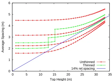
Figure 4: Average (square) spacing over top height, non-logarithmic scales. The slope of the line joining a point to the origin is the relative spacing.
Garc´ıa 2009, Section 4)1. Figure 4 indicates that there is no limiting relative spacing (Hart-Becking or Wilson index). This has been found in other species (Garc´ıa 2009). In fact, Reineke, the 3/2 law, and the Hart-Becking index are mutually incompatible (Section 4).
It may be noted tat the practical significance of these self-thinning models is rather limited, at least for man-aged or planted stands. Most of the interesting stand development occurs far from the limits.
1Actually, this is a mathematical limit as H → ∞, but in reality H has an asymptote of 39.40 m. The slopes cal-culated at this height, for various initial densities N0, are:
N0 125 250 500 1000 2000 4000
3
Stand density management diagrams
SDMDs try to extend the preceding ideas to stands that are not necessarily self-thinning. Following Reineke or the 3/2 law, stand development is shown in logarith-mic axes with number of trees in the abscissa, and mean dbh or mean volume in the ordinate. Sometimes other variables, such as basal area, are used instead of these (Burkhart and Tom´e 2012, Drew and Flewelling 1979, Jack and Long 1996).
10
100 1000
Quadratic Mean DBH (cm)
Trees / ha H = 3 m
H = 4 m H = 5 m H = 6 m
Unthinned Thinned Isolines Slope -1 / 1.6
Figure 5: Predicted LobDyn trajectories graphed as a Reineke-based stand density management diagram.
The same projections from Section 2 were used, except that they were calculated at equal 1 m top height steps instead of 2-year steps. To reduce clutter the graphs do not show ages older than 60 years. Figure 5 displays the predictions in the form of aD-based SDMD. Figure 6 is the analogous for mean tree volume. Points of equal height are joined by so-called isolines. Traditionally, SDMDs de-emphasize the trajectories themselves, rep-resenting them as dotted curves or omitting them alto-gether. Usually, contours are added representing volume or other output variables, that we have not drawn here. Apart from that, the graph for the unthinned stands is similar to a typical SDMD.
SDMDs implicitly assume that the process of remov-ing trees in a thinnremov-ing follows the isolines. There is no
0.001 0.01 0.1 1
100 1000
Mean Tree Volume (m
3 )
Trees / ha H = 3 m
H = 4 m H = 5 m H = 6 m
Unthinned Thinned Isolines Slope -3/2
Figure 6: PredictedLobDyn trajectories graphed as a 3/2-law-based stand density management diagram.
reason why this should be so, and in Figures 5 and 6 the tree size increase estimated by LobDyn for typical thinnings is lower than that implied by the SDMD. In addition, until full occupancy has been restored, growth immediately following a thinning is slower than in un-thinned stands of the same size and density. The error caused by this logical flaw may or may not be acceptable in the practical application of SDMDs, but it should be kept in mind. Garc´ıa (2003) shows similar results based on simulations with the TASS individual-based growth model (Mitchell 1975).
The logarithmic scale makes it difficult to obtain accu-rate estimates over much of the range of interest. With modern computer graphics there seems to be little justi-fication for the historical format, and something like ure 7 might be more useful (Garc´ıa 2003). Or even Fig-ures 8 or 9. Some of the mystique may be lost, though.
4
3-D trajectories and surfaces
0 100 200 300 400 500 600
1 2 3 4 5 6 7 8 9 10
Total Volume (m
3/ha)
Average Spacing (m)
Unthinned Thinned Isolines
Figure 7: A re-scaled SDMD.
0 10 20 30 40 50 60
0 5 10 15 20 25 30
Basal Area (m
2/ha)
Top Height (m) Unthinned
Thinned
Figure 8: Basal areavs. height.
0 100 200 300 400 500 600
0 5 10 15 20 25 30
Total Volume (m
3/ha)
Top Height (m) Unthinned
Thinned
Figure 9: Volumevs. height.
mine the evolution of those two variables. That is a good approximation for unthinned stands, but as discussed above, it can fail when stand development is disturbed. Examining behavior in three dimensions can help to un-derstand better the issues involved. As suggested by Abbott (1884, Section 16), things can seem mysterious when looked at from a low-dimensional space (Figure 10).
Figure 10: Sphere to Flatlander: “See now, I will rise; and the effect upon your eye will be that my Circle will become smaller and smaller till it dwindles to a point and finally vanishes.” (Abbott 1884).
0 5 10 15
20 25 30 0
500 1000
1500 2000
2500 3000
3500 4000
0 10 20 30 40 50 60
DBH (cm)
Unthinned Thinned
Height (m)
Trees / ha DBH (cm)
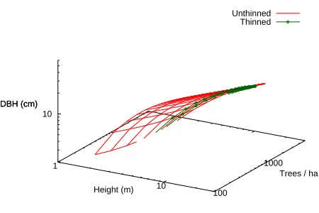
Figure 11: Unthinned trajectories form a 3-D surface. Thin-nings drop somewhat below the unthinned surface.
The LobDyn predictions from Section 3 are repre-sented in an H–N–D space in Figure 11, and with logarithmic coordinates in Figure 12. Any unthinned stand starting at an initial density N0 at breast height
(H = 1.3,D= 0) follows a continuous three-dimensional curve in this space. The set of curves for varying values ofN0form a surface. This observation is completely
gen-eral (at least for a given site quality), and is not specific toLobDyn. Therefore, two state variables are sufficient to describe the dynamics of unthinned stands.
1
10
100
1000 10
DBH (cm)
Unthinned Thinned
Height (m)
Trees / ha DBH (cm)
Figure 12: The surface in logarithmic coordinates.
Figures 2 and 6 are projections into another plane. Many different stand density indices might thus be defined. Clearly, any variables that can be expressed as products of powers of D, N and H could be used, for instance, basal area B∝D2N, or average spacingS∝N−0.5.
Similarly, trajectories, at least those for high densities, can approach a limiting line in the three-dimensional log space. Projections of this line into certain planes generate the various self-thinning lines. Conversely, a two-dimensional self-thinning line defines a perpendicu-lar plane, and two of these planes intersect to generate a three-dimensional limit line. In general, a projection of the 3-D line will not coincide with a third arbitrary 2-D self-thinning line.
Specifically, Reineke’s line is
logN+ 1.6 logD= constant, (1)
and the 3/2 law, assumingv∝D2H, can be written as
2 logD+ logH +3
2logN = constant. (2)
EliminatingD, the projection into logH– logNis found to be
logN+ 4 logH= constant,
which differs from the Hart-Becking-Wilson line
logN+ 2 logH = constant (3)
(Garc´ıa 1993, 2009). It is possible to obtain compati-ble self-thinning lines by changing somewhat the various coefficients, and/or the exponents of the approximation
v∝D2H.
Thinning causes stands to drop below the unthinned surface. Two variables are therefore not longer sufficient for describing the dynamics of managed stands. They might be acceptable as a rough approximation, however.
5
The self-thinning plane
Several authors have noted the existence of a 3-D sur-face, and/or of a limiting “self-thinning plane” in 3-D space (Briegleb 1952, Decourt 1974, Garc´ıa 1988, 1993, O’Hara and Oliver 1988)2. The explanation of Decourt
(1974) assumes stands with different thinning regimes, all starting from the same initial density. O’Hara and Oliver (1988) used age instead ofH, see also Oliver and Larson (1996, Figure 15.1).
By rotating Figure 12, it is found that after canopy closure the surface is close to a plane (Figure 13). This is also suggested by he nearly straight and parallel iso-lines in Figures 5 and 6, although those do not rule-out curvature in the H-direction. “Self-thinning plane” is perhaps not quite accurate, because the approximation is good also for stands not undergoing self-thinning.
An equation for the plane can be obtained by linear regression of one of the log-transformed variables over the other two (excluding young stands for which the approximation does not apply). Or a little more ele-gantly, by finding the direction that minimizes the sum of squared deviations. That direction is given by the co-variance matrix eigenvector with the smallest eigenvalue, or equivalently, by the less significant principal compo-nent (Garc´ıa 1993). Calculating in R (R Development Core Team 2009) using the predicted values withH >6 m,
> x <- log(LobDyn[LobDyn$H > 6, c(’N’, ’H’, ’D’)]) > (y <- eigen(cov(x)))
$values
[1] 1.1392336301 0.2322456491 0.0002257582
$vectors
[,1] [,2] [,3]
[1,] 0.9193056 -0.3069757 -0.2462585 [2,] -0.1541529 -0.8566269 0.4923690 [3,] -0.3620969 -0.4146761 -0.8348230
> summary(as.matrix(x) %*% y$vectors[,3]) V1
Min. :-2.818 1st Qu.:-2.809 Median :-2.800 Mean :-2.797 3rd Qu.:-2.788 Max. :-2.742
> c(y$vectors[,3], -2.797) / y$vectors[1, 3] [1] 1.000000 -1.999399 3.390028 11.357986
Scaled so as to have a unit coefficient for logN, the
1 10 100 1000 10
DBH (cm)
Unthinned Thinned
Height (m)
Trees / ha
DBH (cm) 1
10
100 1000 10
DBH (cm)
Unthinned Thinned
Height (m)
Trees / ha DBH (cm)
Figure 13: Plane approximation.
equation of the plane is
logN−2.00 logH+ 3.39 logD= 11.36. (4)
This is similar to the equation logN − 2.29 logH + 3.28 logD = constant reported for radiata pine per-manent sample plots by Garc´ıa (1993). A principal components fit to Table 2 of Briegleb (1952) gives logN−1.50 logH + 2.78 logD= constant.
Similarly, the values forN0 = 4000 and H >15 give
two eigenvectors with small eigenvalues, corresponding to two planes that intersect to define a three-dimensional self-thinning line. The projections on the standard planes are found to be
logN+ 1.91 logD= constant (5)
2 logD+ logH+ 1.48 logN = constant (6)
logN+ 2.35 logH = constant, (7)
corresponding to equations (1), (2), and (3).
6
Summary and conclusions
Predictions fromLobDynare found to conform reason-ably well to traditional self-thinning “laws”, even though these are not built into the model. Rather than fun-damental biological principles, the rules should be seen as empirical limits that may be acceptable approxima-tions under certain circumstances. In particular, taking an amount of (largely dead) xylem acumulated on the stems, represented by D or v, as a driver or explana-tory variable may be seen as questionable from a physi-ological point of view (Garc´ıa 2009, Garc´ıa et al. 2011). The three conventional laws are not mutually compat-ible, and can be interpreted as plane projections of a three-dimensional line in logarithmic coordinates.
Expected unthinned trajectories are necessarily re-stricted to a surface in three dimensions. This fact can
be useful for understanding the functioning and limita-tions of stand density management diagrams (SDMDs). Thinning causes deviations away from the surface, that are not properly handled by SDMDs. If low accuracy is sufficient, however, these deviations might be consid-ered as relatively small compared to the full range of growing conditions. Almost anything plotted on loga-rithmic coordinates seems to tend to a straight line. On the other hand, the logarithmic scale compression can obscure relevant stand behavior.
In common with previous observations in the litera-ture, LobDyn trajectories approach a three-dimensional “self-thinning plane”.
References
Abbott, E. A., 1884. Flatland: a romance
of many dimensions. Seeley and Co.
(http://archive.org/details/flatlandromanceo00abbou oft).
Beekhuis, J., 1966. Prediction of yield and increment in Pinus radiata stands in New Zealand. Technical Pa-per 49, Forest Research Institute, NZ Forest Service. (http://web.unbc.ca/ garcia/misc/beekhuis66.pdf).
Bi, H., 2001. The self-thinning surface. Forest Science 47(3):361–370.
Briegleb, P. A., 1952. An approach to density measure-ment in Douglas-fir. Journal of Forestry 50:529–536.
Burkhart, H. E., and M. Tom´e, 2012. Modeling Forest Trees and Stands. Springer.
Decourt, N., 1974. Remarque sur une
production. Annales des Sciences Foresti`eres 31:47– 55.
Drew, T. J., and J. W. Flewelling, 1977. Some recent Japanese theories of yield-density relationships and their application to Monterey pine plantations. Forest Science 23(4):517–534.
Drew, T. J., and J. W. Flewelling, 1979. Stand den-sity management: an alternative approach and its ap-plication to Douglas-fir plantations. Forest Science 25(3):518–532.
Garc´ıa, O., 1988. Experience with an advanced growth modelling methodology. In Forest Growth Modelling and Prediction, Ek, A. R., S. R. Shifley, and T. E. Burk, eds., pp. 668–675. USDA Forest Service, Gen-eral Technical Report NC-120.
Garc´ıa, O., 1993. Stand growth models: Theory
and practice. In Advancement in Forest
Inven-tory and Forest Management Sciences — Proceed-ings of the IUFRO Seoul Conference, pp. 22–45. Forestry Research Institute of the Republic of Korea. (http://web.unbc.ca/~garcia/publ/korea.pdf).
Garc´ıa, O., 2003. Dimensionality reduction in
growth models: An example. FBMIS 1:1–15.
(http://cms1.gre.ac.uk/conferences/iufro/fbmis/A/ 3 1 GarciaO 1.pdf).
Garc´ıa, O., 2009. A simple and effective forest
stand mortality model. International Journal
of Mathematical and Computational Forestry &
Natural-Resource Sciences (MCFNS) 1(1):1–9.
(http://mcfns.com/index.php/Journal/article/view/ MCFNS-1:1/44).
Garc´ıa, O., H. E. Burkhart, and R. L. Amateis, 2011. A biologically-consistent stand growth model for loblolly pine in the Piedmont physiographic region, USA. For-est Ecology and Management 262(11):2035–2041.
Jack, S. B., and J. N. Long, 1996. Linkages between silviculture and ecology: an analysis of density man-agement diagrams. Forest Ecology and Manman-agement 86:205–220.
Landsberg, J. J., and R. H. Waring, 1997. A generalized model of forest productivity using simplified concepts of radiation use efficiency, carbon balance and parti-tioning. Forest Ecology and Management 95:209–228.
Leary, R. A., 1997. Testing models of unthinned red pine plantation dynamics using a modified Bakuzis matrix of stand properties. Ecological Modelling 98(1):35–46.
Mitchell, K. J., 1975. Dynamics and simulated yield of Douglas-fir. Forest Science Monograph 17, Society of American Foresters.
Monserud, R. A., T. Ledermann, and H. Sterba, 2005. Are self-thinning constraints needed in a tree-specific mortality model? Forest Science 50(6):848–858.
O’Hara, K. L., and C. D. Oliver, 1988.
Three-dimensional representation of Douglas-fir volume growth: Comparison of growth and yield models with stand data. Forest Science 34(3):724–743.
Oliver, C. D., and B. C. Larson, 1996. Forest Stand Dy-namics. Update edition. John WIley & Sons, Toronto.
R Development Core Team, 2009. R: A Language and Environment for Statistical Computing. R Foundation for Statistical Computing, Vienna, Austria. ISBN 3-900051-07-0 (http://www.R-project.org).
Reineke, L. H., 1933. Perfecting a stand density index for even-aged forests. Journal of Agricultural Research 46:627 638.
Weiskittel, A. R., D. W. Hann, J. John A. Kershaw, and J. K. Vanclay, 2011. Forest Growth and Yield Modeling. Wiley-Blackwell.