A SIMPLE AND EFFECTIVE
FOREST STAND MORTALITY MODEL
Oscar Garc´
ıa
Professor, University of Northern British Columbia, Prince George, BC, Canada. Ph./FAX: 250.960.5004/5539
Abstract. A whole-stand survival model is presented, that is parsimonious and well-behaved when
extrapolated, making it particularly useful in data-poor situations. It is argued, on biological and system-theoretical grounds, that a suitable differential equation for the mortality rate should contain number of trees and top height on the right-hand side, avoiding age, mean diameter, or basal area. Following Eichhorn’s hypothesis, site quality can be neglected by modelling rates relative to height growth. The proposed model is dN/dH =−aNbHc , whereN is number of trees per unit area,H is top height, anda,
band care parameters to be estimated. The equation can be integrated to predict mortality between any two points in time. Satisfactory performance is demonstrated with a white spruce data set from British Columbia. It is shown that the model generalizes concepts of relative spacing, and mortality models for radiata pine and Douglas-fir used by Beekhuis in New Zealand in the 1960’s. Asymptotic behaviour is related to the 3/2, Reineke, and relative spacing self-thinning laws. Limitations of the self-thinning theories and relationships among their various forms are discussed.
Keywords:survival, growth and yield, relative spacing, self-thinning
1
Introduction
The prediction of tree mortality (or more optimisti-cally, survival) is widely recognized as difficult, due to its high variability (e.g., Vanclay 1994). The problem is exacerbated when the available data is limited, and/or does not cover a wide enough range of growing condi-tions. In that situation, it would be desirable to use a model with few parameters, and that behaves reasonably when extrapolated.
I propose such a robust, whole-stand level model for even-aged stands. As usual, catastrophic mortality is ex-cluded, modelling only regular, density-dependent mor-tality (Vanclay 1994). The model has been used as a component in a new stand growth model for natural and planted white spruce in the SBS biogeoclimatic zone of British Columbia; the spruce data is used to illustrate its performance (Figure 1).
The following section presents the reasoning behind the new model, and shows the results of fitting the spruce data. Historically, the model derives from one of Beekhuis (1966), and the connection with it and with concepts of relative spacing are presented next. Finally, relationships to self-thinning theories are discussed.
2
Model
2.1 Rate equations. The mortality rate, for a given site qualityq, can be predicted by some function of the current values of stand variables such as density, age, top height, basal area, mean dbh, volume per hectare, etc.:
dN
dt =−fq(N, A, H, B, D, V, . . .). (1)
Equivalently, models are sometimes expressed in terms of the relative mortality rate (−dN/dt)/N =
−d lnN/dt. Variables such as D and V may enter as part of density indices based on self-thinning laws.
2.2 Stem diameter. Tree diameter, basal area, or volume, reflect the amount of xylem accumulated on the stems. Especially in relatively undisturbed stands, these can be good predictors of future development because they tend to summarize past growth conditions. Biolog-ically, however, a causal connection between the mostly dead xylem and stand development is difficult to justify, and the correlations can be expected to weaken or break down when stand density is manipulated. I suggest that these variables should be avoided on the right-hand sides
Copyright c2009 Publisher of the International Journal ofMathematical and Computational Forestry & Natural-Resource Sciences
0 1000 2000 3000 4000 5000 6000
0 10 20 30 40 50 60 70 80 90
Trees per Hectare
Site-scaled Breast-height Age (years)
Figure 1: British Columbia white spruce stand density data. Re-measurements in each permanent sample plot are joined by lines. A scaling of breast-height age according to site quality makes the trends comparable across sites. All measurements older than 25 years are in natural stands; except for one high-density plot, all the stands younger than 25 years are planted.
of growth models for managed stands. One is left with
dN
dt =−fq(N, A, H). (2)
These models are common. Zhao et al. (2007) re-viewed 27 models that are all of the form
dN dt =−N
af(A, q), (3)
where a is a parameter, andf are various functions of age and site index. Conceptually, it may be useful to distinguish between age, as in A = 33 years-old, and time, as int = 2008. It is convenient, however, to sub-stitute dN/dt= dN/dA, using the fact that dA/dt= 1, i.e., age increases over time at a rate of one year per year. Equation (3) can then be easily integrated as a separable differential equation by writing
N−adN =−f(A, q) dA ,
and integrating on both sides. As a simple example, the model of Clutter and Jones (1980),
dN
dA =−aN
bAc (4)
gives
N1−b
1−b +a
A1+c
1 +c = constant. (5)
The stand density at any age can then be predicted given the density at any other age from
N2= [N11−b−a1−b 1 +c(A
1+c
2 −A1+1 c)]1/(1−b),
provided that there are no management or serious nat-ural disturbances between A1 andA2.
2.3 Age or height? Typically, when a forester looks for explanatory variables, the first one that comes to mind is age. But perhaps he/she is actually thinking of size. For a given site, age and height are closely related, and in practice it may not make much difference which one is used. Physiologically, it can be argued that size would dominate over any ageing effects, especially in
trees, where meristems are constantly renewed. It will Erratum: 7/14/09
be more convenient here to use top height instead of age, so that (2) reduces to
dN
dt =−fq(N, H).
It is also convenient to divide by the height growth equation dH/dt =hq(H), to obtain a relationship be-tweenN andH:
dN
2.4 Eichhorn’s hypothesis. Eichhorn (1904) found that graphing yield table predictions over height instead of age produced similar curves for all site qualities. Al-though not universally accurate, in many instances this so-called Eichhorn’s law is a good approximation (Ass-mann 1970). As a slight extension, the assumption that rates of growth and mortality relative to top height growth are independent of site quality has been success-fully used to simplify the development of growth models (e.g., Beekhuis 1966, Mitchell and Cameron 1985). This hypothesis implies that (6) is approximately indepen-dent of site quality:
dN
dH =−g(N, H). (7)
A model of this form was used by Evert (1981). As an example, Figure 2 shows mortality predictions of Zhao et al. (2007) for loblolly pine with several ini-tial densities and site qualities. Using their site index equation, the same predictions are plotted over domi-nant height in Figure 3. It seems clear that in this case a model like (7) would be satisfactory.
2.5 The model. In view of our objective of estimat-ing mortality with limited data, we want a parsimonious and well-behaved functiong for (7). The chosen model is
dN
dH =−aN
bHc, (8)
where a, b and care parameters to be estimated. Inte-grating gives (cf.equation (5))
N1−b
1−b +a
H1+c
1 +c = constant.
The right-hand side of (8) could be justified as a first-order Taylor expansion of logg in terms of logN and logH, logarithms being used because the original vari-ables are strictly positive. It is analogous to (4), the model of Clutter and Jones (1980), but withH in place of A, making more plausible the independence of site quality.
An alternative formulation and parametrization using average spacing instead ofN may be preferable (Section 3):
Sα−(βH)γ = constant. (9)
Here S = 100/√N is the average square spacing (in meters ifN is number per hectare).
The model limiting behavior is shown below to be compatible with generally accepted theories of self-thinning. The three free parameters provide ample flexi-bility in describing observed trends, but the ratio ofγ/α could also be fixed at reasonable values when dealing with sparse data.
2.6 Application to white spruce. Model (8)–(9) was applied to the data of Figure 1. The parameters were estimated by nonlinear least-squares for the loga-rithm of N (or of S) predicted over pairs of successive
observations. The regression was Erratum: 7/14/09
lnS2= ln[S1α−(βH1)γ+ (βH2)γ]/α , (10) where (H1, S1) and (H2, S2) are consecutive data points. It was felt that the nature of the data did not justify pro-cedures based on more elaborate stochastic modelling.
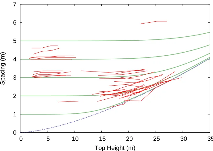
The estimated parameter values wereα= 3.979,β= 0.07213, γ = 6.009. Projections of logN and S are shown in Figures 4 and 5, respectively. The assumption of asymptotic relative spacing (Section 3) resulted in a significantly worse fit, with α=γ= 4.571,β= 0.1004.
3
Beekhuis and relative spacing
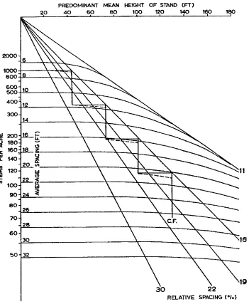
Beekhuis (1966) developed a graphical mortality model for radiata pine plantations in New Zealand that is related to the one in Section 2.5. It was based on rela-tive spacing, the ratio of average spacing to stand height. Relative spacing is sometimes used to specify thinning prescriptions, and is also known as the Hart-Becking or Wilson index (Vanclay 1994, Wilson 1951).
Beekhuis’ model is reproduced in Figure 6. He used triangular average spacing, which is 1.074 times the av-erage square spacing. The graph was constructed assum-ing no mortality until the (triangular) relative spacassum-ing reaches 30%, and the existence of an asymptotic relative spacing of 11%. In between, the spacing–height curve is an arc of ellipse (Garc´ıa 1981). The graph also shows a thinning regime maintaining a relative spacing above 16%. The same technique, with different threshold and limiting relative spacings, was later used in other models for radiata pine and Douglas-fir.
The exact model was rather cumbersome for com-puter implementation, and a close approximation was adopted. Noticing that the slope of theS–H curves de-pends only on the relative spacingR=S/H, increasing from 0 toβ asRdecreases to the limiting relative spac-ingβ, an approximation of the form
dS
dH =R(β/R)
α
was found suitable. Integrating,
Sα−Sα
0 = (βH)α−(βH0)α
(Garc´ıa 1981). With α = 5.5 and β = 0.11 (S be-ing triangular spacbe-ing), the approximation differs from Beekhuis’ curves by less than 3%. This is a special case of (9), withγ=α.
0 100 200 300 400 500 600 700 800 900
0 5 10 15 20 25
Trees / acre
Age (years) Site 60
Site 70 Site 80
Figure 2: Survival projections for loblolly pine plantations in the Piedmont/Upper Coastal Plain, site indices 60, 70, and 80 (Zhao et al. 2007).
0 100 200 300 400 500 600 700 800 900
0 10 20 30 40 50 60 70 80 90
Trees / acre
Dominant Height (feet) Site 60
Site 70 Site 80
100 1000 10000
0 5 10 15 20 25 30
Trees / ha
Top Height (m)
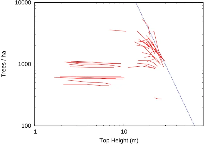
Figure 4: Stand density projections for white spruce from model (8)–(10). LogarithmicN-scale.
0 1 2 3 4 5 6 7
0 5 10 15 20 25 30 35
Spacing (m)
Top Height (m)
through the origin in the S–H plane (Figure 6), rather than to a more general curve as in Figure 5. Unpub-lished work on radiata pine had suggested that the line through the origin did not always look reasonable, and this also seems to be the case with the spruce data (Sec-tion 2.6). The added flexibility of a different γ seems useful, although further research on this topic might be interesting.
4
Self-thinning limits
As mentioned before, our model implies that the S overHtrajectories ultimately approach a limiting curve, which is S= (βH)γ/α. Or, taking logarithms and sub-stitutingN,
logN+ 2γ
αlogH = constant. (11)
This, or more specifically the limiting relative spacing case with γ/α = 1, is an example of self-thinning law
(Figure 7). The other two self-thinning laws commonly encountered in the literature are Reineke’s,
logN+ 1.6 logD= constant, (12)
and the 3/2 law
logw+3
2logN = constant, (13)
whereDis the quadratic mean dbh, andwis mean tree biomass or mean stem volume (e.g., Vanclay 1994).
Although perhaps such “laws” should not be taken too seriously, at least a model that complies with one of them can be trusted to behave reasonably when ex-trapolated. In view of the widespread interest on these topics, however, some additional observations might be relevant.
First, note that the self-thinning line is only an asymp-totic relationship, and does not determine mortality rates over much of the range of interest. In addition, Weller (1987) points out that the distortion caused by the logarithmic transformations, together with the fact that by using an average for diameter or volume the vari-ableN is implicated in both of the graph axes, result in an apparent relationship that is visually stronger than it would otherwise be. To some extent, this idea that self-thinning laws may be partly an optical illusion seems to be supported by a comparison of Figures 1, 4 and 7.
Assumingwapproximately proportional toD2H, (13)
can be expressed in terms of the same variables as (11) and (12):
2 logD+ logH +3
2logN = constant. (14)
An undisturbed forest stand follows some trajectory de-scribing a spatial curve in the three-dimensional space
logD – logH – logN. The self-thinning lines can then be seen as asymptotes for projections of this trajectory on various planes. They can be good approximations for sets of unmanaged stands that do not differ too much in their initial densities, as in the natural stands that have been the subject of most self-thinning research. How-ever, if the stand trajectories are separated due to dif-ferent initial densities or thinning treatments, the most that can be expected is a limiting plane in the three-dimensional space (Bi 2001, Garc´ıa 1993). Projections may still follow (11)–(14), but in general the constant on the right-hand side will vary across stands. Analysis of data from radiata pine plantations (unpublished) has shown reasonable agreement with the limiting slopes of the Reineke and 3/2 laws, but with levels that depend on initial conditions and treatments. Only projections par-allel to the self-thinning plane would produce a unique right-hand side; establishing if (11) is close to one of these would require further research.
Regardless of if the levels vary or not among stands, the slopes of the various self-thinning laws are not nec-essarily compatible (Garc´ıa 1993, Vanclay 1994). Elim-inatingD between (12) and (14) gives
logN+ 4 logH = constant.
This coincides with (11) if γ/α = 2, compared to the
γ/α= 1 of the limiting relative spacing hypothesis. The estimated γ/α = 1.510 from the spruce model can be accommodated by small changes in the nominal coeffi-cients of (12) and (13), and/or in the exponents of the approximationw∝D2H.
5
Conclusions
Limited or poor-quality data requires simple mod-els with guaranteed “logical” behavior. I suggest that dbh, basal area and age should be avoided as explana-tory variables in growth models. Changes relative to height growth are often approximately independent of site quality (Beekhuis 1966, Eichhorn 1904). The mor-tality model of Section 2.5 followed from these principles. The model generalizes and adds flexibility to models used by Beekhuis (1966) and others. Extrapolation pro-duces expected self-thinning patterns. Future research might suggest appropriateγ/α ratios for use when the available data is particularly poor.
Acknowledgments
100 1000 10000
1 10
Trees / ha
Top Height (m)
Figure 7: Self-thinning limiting line for the spruce model. Logarithmic axes.
at UNBC. Useful comments from two anonymous refer-ees are gratefully acknowledged.
References
Assmann, E., 1970. The principles of forest yield study. Pergamon Press, Oxford, England. 506 p.
Beekhuis, J., 1966. Prediction of yield and increment in
Pinus radiata stands in New Zealand. Technical Pa-per 49, Forest Research Institute, NZ Forest Service.
http://web.unbc.ca/~garcia/misc/beekhuis66.pdf.
Bi, H., 2001. The self-thinning surface. Forest Science 47(3):361–370.
Clutter, J., and E. Jones, 1980. Prediction of growth af-ter thinning old-field slash pine plantations. Research Paper SE-217, USDA Forest Service. 14 p.
Eichhorn, F., 1904. Beziehungen zwischen Bestandsh¨ohe und Bestandsmasse. Allg. Forst- u. Jagdztg. 80:45–49.
Evert, F., 1981. A model for regular mortality in unthinned white spruce plantations. The Forestry Chronicle 57(2):77–79.
Garc´ıa, O., 1981. An approximation for Beekhuis’ mortality model. Forest Mensuration Branch Report 57, New Zealand Forest Ser-vice, Forest Research Institute. Unpublished.
http://web.unbc.ca/~garcia/unpub/report57.pdf.
Garc´ıa, O., 1993. Stand growth models: Theory and practice. In Advancement in Forest Inven-tory and Forest Management Sciences — Proceed-ings of the IUFRO Seoul Conference, pp. 22–45. Forestry Research Institute of the Republic of Korea.
http://web.unbc.ca/~garcia/publ/korea.pdf.
Mitchell, K. J., and I. R. Cameron, 1985. Managed stand yield tables for coastal Douglas-fir: Initial density and precommercial thinning. Land Management Re-port 31, B. C. Ministry of Forests, Research Branch, Victoria, British Columbia.
Vanclay, J. K., 1994. Modelling forest growth and yield: Applications to mixed tropical forests. CABI International, Wallingford, UK. 312 p.
http://espace.library.uq.edu.au/eserv/UQ:8211 /ModellingForestG.pdf.
Weller, D. E., 1987. A reevaluation of the -3/2 power rule of plant self-thinning. Ecological Monographs 57:23– 43.
Wilson, F. G., 1951. Control of stocking in even-aged stands of conifers. Journal of Forestry 49:692–695.
Biographical Note
Oscar Garc´ıa is a Professor and Endowed Chair in Forest Growth and Yield at the University of North-ern British Columbia, Canada. He received a profes-sional forester degree (Ingeniero Forestal) and an M.Sc. in Mathematical Statistics & Operations Research from the University of Chile, and a Ph.D. in Forest Resources from the University of Georgia, USA. Between 1976 and 1992 he worked in New Zealand for the Forest