www.theoryofcomputing.org
How Hard Is It to
Approximate the Jones Polynomial?
Greg Kuperberg
∗Received August 5, 2009; Revised October 27, 2014; Published June 6, 2015
Dedicated to the memory of François Jaeger (1947-1997)
Abstract: Freedman, Kitaev, and Wang (2002), and later Aharonov, Jones, and Landau
(2009), established a quantum algorithm to “additively” approximate the Jones polynomial V(L,t)at any principal root of unityt. The strength of this additive approximation depends exponentially on the bridge number of the link presentation. Freedman, Larsen, and Wang (2002) established that the approximation is universal for quantum computation at a non-lattice, principal root of unity.
We show that any value-distinguishing approximation of the Jones polynomial at these non-lattice roots of unity is #P-hard. Given the power to decide whether|V(L,t)|<aor |V(L,t)|>bfor fixed constants 0<a<b, there is a polynomial-time algorithm to exactly count the solutions to arbitrary combinatorial equations. Our result is a mutual corollary of the universality of the Jones polynomial, and Aaronson’s theorem (2005) thatPostBQP=PP. Using similar methods, we find a range of valuesT(G,x,y)of the Tutte polynomial such that for anyc>1,T(G,x,y)is #P-hard to approximate within a factor ofceven for planar graphsG.
Along the way, we clarify and generalize both Aaronson’s theorem and the Solovay-Kitaev theorem.
ACM Classification:F.1.3, G.2.2
AMS Classification:68Q17, 68Q12, 57M27, 05C31
Key words and phrases:hardness, quantum computation, Jones polynomial, Tutte polynomial
1
Introduction
A well-known paper of Aharonov, Jones, and Landau [5] establishes a polynomial quantum algorithm to approximate the Jones polynomial at any principal root of unity; a more abstract form of this algorithm appeared previously in a paper of Freedman, Kitaev, and Wang [11].
Theorem 1.1(Freedman, Kitaev, Wang [11]; Aharonov, Jones, Landau [5]). Let t=exp(2πi/r)be a
principal root of unity, let L be a link presented by a plat diagram with bridge number g, and let V(L,t)
be its Jones polynomial. Then there is a polynomial-time quantum decision algorithm that answers yes with probability
P[yes] =
V(L,t) (t1/2+t−1/2)g−1
2 .
(See Burde and Zieschang [9, §2.D] orSection 3.4for the definition of a plat diagram and its bridge number.)
In the version of the result of Aharonov et al., the algorithm is jointly polynomial time in ther, the order of the root of unity; as well as in the bridge number and the crossing number. They also refine the algorithm to estimateV(L,t)as a complex number rather than just estimating its length. Aharonov et al. describe the error in this algorithm as additive, and note that it would be much harder to provide an algorithm with multiplicative error. Multiplicative approximation (in the sense of the complexity class APX[40]) would mean thatV(L,t)or|V(L,t)|can be approximated to within some constant factorc>1. Another way to distinguish between types of error is to say that the approximation inTheorem 1.1
isinput-dependent. Given different plat diagrams of the same linkL, the error grows exponentially in one of the parameters of the presentation, namely the bridge number. (This additive, input-dependent model of approximating the Jones polynomial was first considered in the converse problem of simulating a quantum computer with the Jones polynomial [7].) An algorithm to approximate the Jones polynomial is only directly useful for topology if the approximation isvalue-distinguishing; i. e., if there is an error bound which is independent of quantities other than the value of|V(L,t)|. Multiplicative approximation is one type of value-distinguishing approximation, but it is not the most general kind. For instance, a multiplicative approximation of log(1+|V(L,t)|)is much weaker than a multiplicative approximation of|V(L,t)|itself, but it is still a value-distinguishing approximation. In general, if an algorithm yield any value-distinguishing approximation of a real-valued function f(x), it means that for eachc∈R, there exist real numbersa<c<bsuch that f(x)<acan be distinguished from f(x)>b. (See also
Section 2.2.)
Freedman, Larsen, and Wang [13] established that the approximated quantity
V(L,t)/ t
1/2+t−1/2g−1
2
These results show that even if the approximation is input-dependent, it is computationally valuable for carefully chosen link diagrams.
On the discouraging side, Vertigan [36] showed that it is #P-hard to exactly compute the Jones polynomialV(L,t)except whentis a lattice root of unity. Jaeger, Vertigan, and Welsh [20] established a reduction from the Tutte polynomial of a planar graph to the Jones polynomial of an associated link. Vertigan then showed that the specific values of the Tutte polynomial used in this reduction are #P-hard. The main result of this article is that the “encouraging” universality result strengthens the “discourag-ing” hardness result: Any value-distinguishing approximation of a value of the Jones polynomial at a non-lattice root of unity is #P-hard. The argument is a mash-up of three standard theorems in quantum computation: The Solovay-Kitaev theorem [30], the FLW density theorem, and Aaronson’s theorem that PostBQP=PP[1]. (See also [7] for a different hardness result.)
Theorem 1.2. Let V(L,t)be the Jones polynomial of a link L described by a link diagram, and let t be a
principal, non-lattice root of unity. Let0<a<b be two positive real numbers, and assume as a promise that either|V(L,t)|<a or|V(L,t)|>b. Then it is#P-hard, in the sense of Cook-Turing reduction, to decide which inequality holds. Moreover, it is still#P-hard when L is a knot.
Theorem 1.2is proven in Section 3.5after developing several lemmas. The theorem is stated for the Jones polynomial and only for values where the associated braid group representations are unitary and dense. But the idea applies to many other link invariants and to many non-unitary values of the Jones polynomial. The idea also applies to various functions on graphs or other input data that aren’t link invariants. We have no formal statement of a general result, but the basic argument is that if a numerical function can model the execution of a quantum computer sufficiently accurately, then typically multiplicative or value-distinguishing approximation is universal forPostBQPand therefore #P-hard. Here is an example result of this type.
Theorem 1.3. Let c>1and let x and y be two real numbers such that q= (x−1)(y−1)>4and
x,y<0, and x and y each have anFPTEASapproximation. Then it is#P-hard to approximate the Tutte polynomial value T(G,x,y)for planar graphs G to within a factor of c.
Here, a real or complex number has anFPTEAS(fully polynomial-time exponential approximation scheme) if its digits can be computed inFP, for instance if it is an algebraic number (Section 2.2). One interesting ingredient is that we need the Solovay-Kitaev theorem for non-compact Lie groups,
Theorem 2.4. (Aharonov, Arad, Eban, and Landau [4] obtained this result for the Lie groups SL(d,R) and SL(d,C), which is actually enough forTheorem 1.3.)
We will complete proveTheorem 1.3inSection 4.5, again after developing some lemmas.
In related results, Aharonov, Arad, Eban, and Landau [4] obtainedBQP-universality results about additive approximation to the Tutte polynomial for planar graphs that are clearly related toTheorem 1.3. In particular, as with us, their approach involves a study of non-unitary linear gates. However, their derivation concerns multivariate Tutte polynomials, in which different edges of a graph are allowed different parameters. The value ofqmust be the same everywhere, but in their version the choice ofx (say) is taken from a finite list that satisfies technical conditions. Following Goldberg and Jerrum, we restrict to a single pair of values(x,y).
values (those withq=4 and−1<y<0) are #P-hard. Jaeger, Vertigan, and Welsh [20] also analyzed whenT(G,x,y)is #P-hard to compute exactly. They noted that the Jones polynomialV(L,t)of an alter-nating linkLis equivalent toT(G,x,y)for a planar graphGalong the curvexy=1. More recently [16], Goldberg and Jerrum also established that many values of the planar Tutte polynomial areNP-hard to approximate. Their new theorems apply to those values of(x,y)inTheorem 1.3withq>5 (and some other values that we do not analyze), but their constructions are very different. Moreover, we establish #P-hardness, while their planar constructions only establishNP-hardness. On the other hand, we use Goldberg and Jerrum’s gadget idea to change from one value of(x,y)to another for a fixed value ofq.
Remark 1.4. The first version of this article contained a significant mistake, which the reader may
grasp after readingSection 2.5. The author supposed that all of the implementations of quantum gates could have complexity poly(1/ε)(or FPTASapproximability) in the proof of bothTheorem 1.2and
Theorem 1.3, because this complexity is sufficient to express the complexity classBQP. We actually need complexity poly(−log(ε))(orFPTEAS) to express the complexity classPostBQP, because this class unavoidably needs exponentially small probabilities. Fortunately, the Solovay-Kitaev theorem (Theorem 2.4) satisfies this stringent approximation requirement. See alsoLemma 4.3andTheorem 2.10
for our corrected constructions.
Acknowledgments
The author would like to thank Scott Aaronson, Dorit Aharonov, Leslie Ann Goldberg, and Eric Rowell for helpful discussions. The author would also like to thank the referees for their meticulous remarks.
2
Complexity theory
2.1 Complexity classes
We assume that the reader is somewhat familiar with complexity classes such asP,NP,BQP, #P, and the notation thatAB means the classAwith oracleB. See the Complexity Zoo [40] and Nielsen and Chuang [30] for a review.
Whereas a problem in the class #Pcounts the number of witnesses accepted by a verifier in polynomial time, and a problem the classNPreports whether there is an accepted witness, a problem in the classPP reports whether a majority of the witnesses are accepted.
Proposition 2.1. A problem is#P-hard if and only if it isPP-hard with respect to Cook-Turing reduction,
i. e.,
PPP=P#P.
A problem which is #P-hard is also hard for the polynomial hierarchyPH, by the deeper theorem due to Toda [34] that
PHdef=
∞
[
n=1
NPNP. .
.NP
| {z }
n
⊆P#P.
The classNPwith a tower ofn−1NPs as an oracle is called thenth level of the polynomial hierarchy. One of the standard conjectures in complexity theory is the polynomial hierarchy does not collapse, i. e., thatnth level does not equal then+1st level for anyn. Thus by Toda’s theorem, if a problem is #P-hard, then it is viewed as qualitatively harder than if it is merelyNP-hard.
2.2 Approximation classes
The approximation classes listed in the Complexity Zoo [40] that express multiplicative approximation includeAPX,PTAS, andFPTAS. These classes are defined there for optimization problems, but they can equally well be defined for arbitrary functional problems. Let f:Σ∗→R+ be a function that takes
bit stringsxto positive real numbers. Then f(x) is inAPX if it can be approximated to within some bounded factor in polynomial time (with fixed-point output); it is inPTASif it can be approximated to within a factor 1+ε in polynomial time for anyε>0; and it is inFPTASif the computation is jointly polynomial time in the bit length|x|and 1/ε. (These classes all refer to deterministic computation; there are analogous randomized classes such asFPRAS.)
We will need a stricter version ofFPTAS. For many approximate numerical algorithms, although not usually for optimization problems, the computation time is jointly polynomial in|x|and−log(ε). We call such an approximation scheme anFPTEAS, orfully polynomial time, exponential approximation scheme. In particular every algebraic number has anFPTEAS, using standard numerical algorithms to find its digits.
Indeed, much more is true: The digits of algebraic numbers, and the values of many other elementary functions such as exponentials and logarithms, can be computed in quasilinear time in the RAM machine model [8]. Most numbers that arise in calculus derivations have quasilinear digit complexity; nearly all of them have polynomial digit complexity.
We do not know of a standard complexity class to express general value-distinguishing approximation, so we define such a class here,APV. Again let f:Σ∗→R+. Then f is inAPVif for every constanta>0,
there exists a constantb>aand a polynomial-time algorithm to decide whether f(x)>bor f(x)<a, given the promise that one of the two is true. Similarly, we could define a randomized versionARV. Also, bothAPVandARVhave a variation in which the constantais an input to one universal algorithm, instead of asking for an algorithm for each value ofa.
The following proposition says that if f(x)can be suitably rescaled, then general value-distinguishing approximation becomes equivalent to multiplicative approximation in the sense ofAPX.Proposition 2.2
and its proof are similar to that ofProposition 2.14, in particular similar to the rescaling of Aaronson [1, Thm 3.4]. We will need the contrapositive ofProposition 2.2in the proof ofTheorem 1.2.
Proposition 2.2. Suppose that f(x)takes positive real values and is inAPV, and suppose further that
c>1and k>1such that for every integer n, there is a reduction yn(x)such that f(x)<knf(yn(x))<c f(x),
and suppose that this reduction can be computed in joint polynomial time in n and in|x|. Then f(x)is in APX.
Proof. Let aand bbe some constants such that we can decide by a subroutine whether f(x)<a or f(x)>bin polynomial time. Then we can bound f(x)to within a factor ofcb/a. We know by hypothesis that f(x)>k−mand f(x)<kmfor somemwhich is polynomial in|x|. So the strategy is to ask whether f(yn(x))is less thanaor more thanbfor every|n| ≤m. The largestnfor which the subroutine reports that f(yn(x))<ayields a good estimate ofak−n. The estimate is within a factor ofcb/a, even though the subroutine could give a false yes answer when f(yn(x))>b.
2.3 Quantum computation
We cannot give a full review of quantum computation in this article. There are many equivalent models of quantum computation, and we would simply like to carefully describe the one that we will use. Let D:Σ∗→ {yes,no}be a decision problem, a functionD(x)on bit stringsxthat takes the values “yes” and
“no.” In the most standard definition ofBQP, we assume a uniform family of quantum circuitsCsuch thatxis supplied in input qubits along with ancillas, and one of the output qubits is the outputD(x)with good probability. We will use a variation of this definition in which the input is encoded in the circuit rather than in the input to its gates; and the inputs and outputs are all set to 0.
Proposition 2.3. D∈BQPif and only if there is a quantum circuit C=C(x)withpoly(|x|)unitary gates acting on n=poly(|x|)qubits, such that C itself can be generated in deterministic polynomial timeFP, and such that the probability
p(x) =|h0n|C|0ni|2 (2.1)
is at least2/3if D(x) =yesand at most1/3if D(x)isno.
Proposition 2.3is a well-known result even though it is not the most standard definition. The proof uses the “uncomputation” method.
Proof. We first assume a circuitC=C(n)of the more standard type in which|xiis the input along with |0iancillas, and one of the qubits is the output. Then we can make a new circuitC0whose input is all ancillas, and that first changes some of the ancillas to|xi. One of the outputs|yiofC0agrees withD(x)
with probability at least 2/3; the other outputs are unpredictable. We make a new circuitC00that applies C0, then copies|yito a fresh ancilla with a CNOT gate, and then applies(C0)−1.
2.4 Solovay-Kitaev
and can be calledBQP. We need some approximability condition here: If the matrix entries of gates in
Γhave intractable or uncomputable information, thenBQPΓalso carries intractable or uncomputable information [2, Thm. 5.1].
In this paper we will need the more delicate classPostBQP. As stated inTheorem 2.10, in order to know thatPostBQPΓis independent ofΓ, we need to assume that every gate inΓhas anFPTEAS, and not just anFPTAS. One special case which is widely used in quantum computation and which we need forTheorem 1.2is gates with algebraic entries; happily, all algebraic gates have anFPTEAS. (Indeed theFPTEASclass is far more general, as explained inSection 2.2.) We also need the Solovay-Kitaev theorem to have polylogarithmic overhead; happily it does.
Finally, forTheorem 1.3we will need the Solovay-Kitaev theorem for non-compact Lie groups. The theorem was originally proven in the caseG=SU(d). This case is explained in Nielsen and Chuang [30]; as far as we know the proof works without change whenGis any compact, semisimple Lie group. Aharonov, Arad, Eban, and Landau [4] derive a version of this theorem for the Lie groups SL(d,R)and SL(d,C), which are not compact but still semisimple. Their result is enough forTheorem 1.3; here we show that the traditional argument applies to a more general class of Lie groups.
Theorem 2.4(Solovay, Kitaev). Let G be a connected Lie group whose Lie algebragis perfect. Let
Γbe a finite set of elements (closed under taking inverses) that densely generates G, and let g∈G.
Suppose that there is anFPTEASfor g and every element ofΓ. Then there is a word made fromΓthat approximates g,
d(g1g2. . .gm,g)≤ε,
where the length m and the (deterministic) computation time to find the word are bothpoly(−log(ε)) (non-uniformly in the choice of G,Γ, and g).
Before turning to the proof ofTheorem 2.4, we discuss some basics of Lie theory. (See Varadara-jan [35].)
A Lie groupGis a real analytic manifold with a real analytic group law. (Or a smooth manifold or even just a topological manifold; it turns out that the group law induces a unique real analytic structure.) Its Lie algebrag=T1Gis by definition the tangent space at the identity. We assume that our Lie group Gis given with some tractable algorithm for computing the group law in real analytic coordinates. For example,Gcould be a real algebraic group, by definition a Lie group that can be realized (non-uniquely) by polynomial equations in some GL(n,R).
We can giveG a metric to discuss approximation to points in G. The most natural choice is a left-invariant Riemannian metric [31]. Every left-invariant Riemannian metric comes from a positive definite inner product on the Lie algebragofG. Two different inner products ongplainly yield different Riemannian metrics onG, but they are they are bi-Lipschitz equivalent. (Ifd1andd2are two metrics on a set, then they arebi-Lipschitz equivalentifd1(p,q) =Θ(d2(p,q)).) A left-invariant metric on GL(n,R)is not bi-Lipschitz equivalent with Euclidean distance between matrices, but it is equivalent on any bounded set. Thus, any of these choices of metric are equivalent for the purpose of statingTheorem 2.4.
analogous to a finite perfect group.) The most commonly used Lie algebras, such assu(d)andsl(n,R), have simple and therefore semisimiple Lie algebras (and are themselves called semisimple groups). Every semisimple Lie algebra is perfect, but there are perfect Lie algebras that are not semisimple. For example, ifV is a linear representation of a semisimple Lie groupGwithout any trivial summand, then the Lie algebra of the semidirect productGnV is perfect.
Every Lie groupGhas a (real analytic)exponential map exp :g→G defined in polar coordinates by the derivative equation
d
dtexp(tx) =xexp(tx)
fort∈R≥0andx∈g. In the special case of an algebraic group, it is the usual matrix exponential. We will use three standard results about the derivative map. To state the results, we assume some inner product on
g, and the induced left-invariant metric onG.
Proposition 2.5([35, Thm. 2.10.1]). The exponential mapexpis a bi-Lipschitz, diffeomorphic embedding
when restricted to a ball B=B(0,ε)of some radiusε ing.
Proposition 2.6([35, Thm. 2.10.1]). Suppose thatghas a basis b1, . . . ,bk, and define a function h:g→G by
h
∑
j tjbj
!
=
∏
j
exp(tjbj).
Then f is a bi-Lipschitz embedding when restricted to a ball B=B(0,ε)of some radiusε ing. Moreover, we can chooseεandδ so that f is uniformly bi-Lipschitz for any basis b01, . . . ,b0k withkb0
j−bjk<δ.
Proposition 2.6 is less standard than Proposition 2.5, but happily Varadarajan proves a mutual generalization in a single theorem. The last statement about uniform constants if the basis{bj} is perturbed is not in the statement of the theorem, but it follows readily from the proof. Remark: The formula inProposition 2.6is a generalization of Euler angles for the group SO(3).
Proposition 2.7([35, Thm. 2.12.4]). If[g,h]G=ghg−1h−1is the group commutator and[x,y]gis the Lie bracket, then
[exp(x),exp(y)]G=exp([x,y]g+O max(kxk,kyk)3)
.
Varadarajan provesProposition 2.7with a less uniform error estimate, but the same proof establishes the given formula.
Since the result is not required to be uniform ing, we do not need a global epsilon net of the Lie groupG, only a local one near the identity; a global epsilon net would add extra difficulties in the non-compact case. Another trick that simplifies the derivation is to save the choice ofrfor the end; it also serves as a fudge factor to enable the construction.
Proof ofTheorem 2.4. Let k be the dimension ofG. If gis a perfect Lie algebra, then it has a basis b1, . . . ,bk and elementsx1, . . . ,xkandy1, . . . ,yksuch that[xj,yj] =bj. We choose some positive definite inner product ongand take the induced left-invariant Riemannian metric onG.
ByProposition 2.5, the exponential map exp :g→Gis a bi-Lipschitz diffeomorphism within some radiusε1. Also, letε2andδ be the constants produced byProposition 2.6, a radius out to which the map f is a bi-Lipschitz diffeomorphism. Also, since the Lie bracket is bilinear, and by the approximation inProposition 2.7, we can choose a radiusε3 within which both the Lie bracket ong and the group commutator onGtake the ballB3=B(0,ε3)to itself. In other words, both brackets are maps
[·,·]g:B3×B3→B3 and [·,·]G: exp(B3)×exp(B3)→exp(B3) whenε3is small enough. Finally we choose
ε0=min(ε1,ε2,ε3)
to obtain all three properties simultaneously, and we letB0=B(0,ε0).
We take advantage of a subtlety ofProposition 2.6, that the maphonly depends on the lines spanned by{bj}. We can thus rescale the vectors{xj,yj,bj} so that they all lie inB0, without disturbing the constants used to defineB0.
We can interpret the group commutator[·,·]Gas a map fromB0×B0toB0via the equation
[x,y]G def
=log [exp(x),exp(y)]G
so that we can then say restateProposition 2.7as saying that
[x,y]G= [x,y]g+O max(kxk,kyk)3
. (2.2)
Without loss of generality,g∈exp(B0): BecauseΓdensely generatesG, we can find a word close to
gand multiplygby its inverse. Also, we letr<1 be a constant that will be chosen at the end of the proof. Again becauseΓdensely generatesG, we can assume for eachn≤3 that it contains the set{exp(bj,n)} for a basis{bj,n}inB0such that
kr−n
bj,n−bjk<δ (2.3)
for every j. Recall again thatδ is chosen to matchProposition 2.6.
In the remainder of the proof, we will use asymptotic notation such asx=O(r)to express errors in Lie elementsx∈g. What we mean is thatkxk<Cr, where each constantCdoes not depend onrorn, but can depend on everything else defined so far.
For each integern≥1, we want to define Lie algebra elementsbj,n,xj,n, andyj,n, all of them words inΓmade using the group law ofG, such that (2.3) holds for alln, and such that
also holds for alln. The definition is by an inductive algorithm that makesxj,nandyj,nfrombj,n+1, and makesbj,n fromxj,dn/2eandyj,bn/2c. So the numbering innis slightly out of order, but since we have
already producedbj,nforn≤3, the induction works.
For eachn≥1, we choose integerstj=O(r−1)so that the expressions
log
∏
jexp(tjbj,n+1)
!
(2.5)
are as close as possible tornxjandrnyj. We setxj,nandyj,nto be these approximations. We claim that the expressions in (2.5) form anO(rn+1))-net ofrnB0. We argue this in stages:
1. The sums∑jtjrn+1bjare a lattice and anO(rn+1)-net by rescaling.
2. The sums∑jtjbj,n+1are anO(rn+1)-net because (2.3) limits the distortion of the lattice.
3. The products∏jexp(tjbj,n+1)are anO(rn+1)-net because the maphinProposition 2.6is Lipschitz onB0.
4. The logarithms
log
∏
jexp(tjbj,n+1)
!
are anO(rn+1)-net because the exponential map exp is inverse Lipschitz onB0. Thus, we obtain the error estimates (2.4).
For eachn≥4, we let
bj,n= [xj,dn/2e,yj,bn/2c]G. If we combine (2.4) with (2.2), we obtain
bj,n=rn(bj+O(r) +O(r3bn/2c−n)) =rn(bj+O(r)). (2.6) We would like to reconcile (2.6) with (2.3). The relation (2.6) gives us
kr−nbj,n−bjk<Cr
and we are done provided thatCr<δ. So, at final this stage it is crucial thatCdoes not depend onnorr; we can choosersmall enough to make the induction work.
Finally we letg0=g∈exp(B0). We inductively let hn=
∏
j
exp(bj,n+1)tj
as in (2.5), and then we letgn+1=h−n1gn. We obtain the estimate klog(gn+1)k=O(rn+1).
Theorem 2.4is not uniform in the choice of the group elementgand we do not need this uniformity for our purposes. However, the proof shows that it is uniform on any bounded region inG. For completeness, we give a complementary result that in any semisimple algebraic group, any element can be efficiently approximated to within a bounded distance.
Theorem 2.8. Let G be a semisimple (real) algebraic group which is equipped with a left-invariant
Riemannian metric, and which is densely generated by a subsetΓ. Let r>0, let g∈G, and let`=d(g,1).
Then there is word made fromΓthat approximates g to within a bounded distance, d(g1g2. . .gm,g)<r
with m=O(`+1)uniformly in g. Moreover, such a word can be found in timepoly(`). EvidentlyTheorem 2.8can be combined withTheorem 2.4to obtain a total word length of
m=O(`+1) +poly(−log(ε)).
Note also that the lower boundm=Ω(`+1)follows from the triangle inequality
d(1,gh)≤d(1,g) +d(1,h)
and the fact that the finite setΓhas a maximum distance to 1. SoTheorem 2.8is optimal up to a constant factor.
We conjecture thatTheorem 2.8holds for all connected Lie groups. Note that most named Lie groups, such as GL(n,R),O(n,C), etc., are algebraic groups.
Proof. We assume thatGis given as a subgroup of some GL(n,R)defined by polynomial equations. We review some of the structure theory of semisimple real algebraic groups [31]:
1. Ghas a maximal compact subgroupK.
2. Every elementg∈Ghas a (canonical) Cartan decompositiong=exp(x)k, wherek∈Kandx∈k⊥⊆g. 3. The quotient manifoldG/Khas aG-invariant Riemannian metric; it is then called asymmetric space
of noncompact type.
4. In the quotientG/K, the unique geodesic connectinggK=exp(x)Kto the identity coset is given by exp(tx)Kwith 0≤t≤1.
5. Up to a change of basis,G=GT, i. e.,Gis stable under the transpose map.K=G∩O(n)is a maximal compact subgroup if and only ifG=GT.
Note also that everyG-invariant metric onG/K comes from a left-invariant metric onGwhich also happens to be right-K-invariant. We assume such a metric onG. As a consequence, given any two group elementsg,h∈G, we have both that
d(gK,hK)≤dG(g,h)
and that equality can be achieved by passing to a different representativeg0∈gK orh0∈hK. (We need not change both.)
The idea of our proof is to first find a word with all of the desired properties in the symmetric space G/Krather than in the groupG. The advantage of working inG/Kis that we know how to calculate geodesics and distances, using polar decompositions. Geometrically, the idea is not complicated: We can build a word by taking steps approximately in the direction of the geodesic from 1KtogK.
SinceΓdensely generatesG, and since closed and bounded regions inGare compact, we can assume
without loss of generality thatΓcontains anr/2-net of points inside the closed ballB=B(1,r)of radius rat the identity. GivengK∈G/K, letγbe the unique geodesic that connects 1KtogK; we can compute it from the polar decomposition ofg. LethK be the point at whichγexitsBK. Then we know or we can assume that
d(1K,hK) =d(1,h) =r and d(hK,gK) =d(h,g) =`−r. We can chooseg1∈Γsuch thatd(g1,h)<r/2. By the triangle inequality,
d(g1,g) =d(1,g−11g)< `− r 2.
Thus, we can letg0=g−11gand proceed by induction.
We obtain a wordwsuch thatd(w−1g,K)<r/2. We are given thatKis compact; it follows that there is a finite set of wordsvinΓthat forms anr/2-net ofK. So for one of these words,
d(wv,g) =d(v,w−1g)< r 2+
r 2 =r as desired.
2.5 Postselection
Aaronson [1] defined the classPostBQPas polynomial-time quantum computation with free retries, or postselection. In other words, the computation can output|yesi,|noi, or|retryi. (In Aaronson’s formal definition, the outputs are measured ash00|,h01|, andh1∗ |, respectively; of course the output can equally well be a qutrit whose values are renamed semantically.) If the absolute probabilities are
P[yes] =a and P[no] =b then the conditional or postselected probabilities are
P[yes|yes or no] = a
An algorithm inPostBQPis required to output “yes” or “no” with conditional (rather than absolute) probability of at least 2/3. It is trivially equivalent to say that for somec>1, eithera>cborb>ca; all values ofcare equivalent becauseccan be amplified by repeated trials. There is an analogous class PostBPPfor classical randomized computations; it was also defined previously asBPPpath. Aaronson established thatPostBQP=PP. It is not hard to show thatPostBQPis a subset ofPP, just asBQP,NP, and a number of other important classes are known to be. (The inclusionSBQP⊆A0PPis proved in the same way inProposition 2.13.) The more surprising fact is thatPostBQPis all ofPP.
By contrast,PostBPPis unlikely to be all ofPP. The relevant complexity results are as follows:
1. PostBPPcontainsP||NP(Pwith parallelNPqueries) [17].
2. P||NPequalsPNP[log](Pwith logarithmically manyNPqueries) [19,10].
3. PostBPPderandomizes toP||NP. I. e., they are equal if sufficiently good pseudo-random number generators exist [33].
4. Without any derandomization assumption [17],
PostBPP⊆BPPNP⊆NPNPNP.
Thus,PostBPPis known to be in the third level ofPH. If we accept derandomization, then it is in the second level.
Another interpretation ofPostBQPorPostBPPis given by the following proposition:
Proposition 2.9. Let c>1. Then a decision function D is inPostBPP if and only if there are two
randomized, polynomial time algorithms run by Alice and Bob that report “yes” with probabilities a and b, and such that D(x) =yeswhen a>cb and D(x) =nowhen b>ca. The same holds forPostBQPand quantum algorithms.
Proof. Suppose that we are given aPostBQPalgorithm in the original definition. Then Alice and Bob can both run this algorithm, with the following conversion:
yes7→Alice yes, Bob no,
no7→Alice no, Bob yes, retry7→Alice no, Bob no.
It is easy to check that this satisfies the requirements of the proposition. Conversely, suppose that Alice and Bob have separate algorithms. Then we can combine them into one postselecting algorithm in Aaronson’s sense by flipping a coin to decide which of Alice or Bob runs; only one of them runs in a given trial. We can convert according to the following table:
Alice yes7→yes, Alice no7→retry,
Bob yes7→no, Bob no7→retry.
We also need to clarify the definition ofPostBQPwith regard to different gate sets. Aaronson defines PostBQPusing Hadamard and Toffoli gates, on the argument that all choices of gates are equivalent by Solovay-Kitaev. But this is somewhat overstated; we give a more precise equivalence as follows:
Theorem 2.10. LetΓbe a universal gate set acting on qudits, letPostBQPΓbePostBQPdefined with
the gate setΓ, and suppose that:
1. The matrix entries in each gate have anFPTEAS.
2. If z6=0is expressible as an integer polynomial in the gate entries with bit complexitypoly(n)with exponents written in unary, then
|z|>exp(−poly(n)).
ThenPostBQP=PostBQPΓ. If only condition 1 holds, thenPostBQP⊆PostBQPΓ.
Before provingTheorem 2.10, here are three remarks. First, the classBQPonly requires a weaker version of condition 1, namely that each gate inΓhas anFPTAS, in order to enable the Solovay-Kitaev
theorem. We needFPTEASbecause PostBQPrelies on exponentially small probabilities. Without exponentially good approximation, Solovay-Kitaev would still give us a circuit reduction, but the reduction would be relative toP/poly rather than relative to P. Second, we conjecture that if only condition 1 holds, thenPostBQPandPostBQPΓare not always equal. Third, we do not know whether postselected quantum computation is gate-independent with a time bound of ˜O(nα) for some fixed
exponentα, because the Solovay-Kitaev theorem could change the exponent.
Proof. Condition 1 andTheorem 2.4together imply thatPostBQP⊆PostBQPΓ. The traditional gate set consisting of Hadamard and Toffoli gates can be approximated using gates inΓ; how good of an
approximation is sufficient? It is easy to check that the Hadamard and Toffoli gates satisfy condition 2, so the strength of approximation that we need is exp(−poly(|x|)). This is precisely how muchTheorem 2.4
gives us with polynomial overhead, if each gate inΓhas anFPTEAS.
The same argument works in reverse, but we must add condition 2 explicitly, since it is not guaranteed in general.
We will not strictly need the following proposition, but it helps for understandingTheorem 2.10. It shows that any gate set with algebraic matrix entries automatically satisfies condition 2.
Theorem 2.11. Let t1, . . . ,tkbe a finite list of algebraic numbers inC, and let p be an integer polynomial in k variables with bit complexitypoly(n)with exponents written in unary. Then
|p(t1, . . . ,tk)|>exp(−poly(n)) (non-uniformly in the choice of{tj}), assuming that the value is non-zero.
fixed polynomials can be composed with the polynomial pin the proposition. Thus, without loss of generality, we can takek=1 andt=t1.
Next we consider the case thatt=a/b∈Qis rational. In this it is enough for pto have degree poly(n), because we immediately get
|p(t)|>bdegp.
In the general case, letdbe the degree of the fieldK, and letz=p(t). Thenz=z1has a list of Galois conjugatesz1,z2, . . . ,zd. Moreover, if we choose some basis of the ring of integers ofK, thenthas rational coordinatess1, . . . ,sd, and we can write
d
∏
j=1
zj=q(s1, . . . ,sd)
for a polynomialqwith degq=d(degp). Thus by the rational case we obtain
d
∏
j=1 zj
>exp(−poly(n)).
At the same time, because of the degree bound onpand because each coefficient of pis bounded by exp(poly(n)), we obtain
|zj|<exp(−poly(n)). By dividing through, we obtain
|z|=|z1|>exp(−poly(n)).
It is important to compare PostBQPand PostBPP to three other complexity classes: A0PP, or one-sided almost widePP, defined by Vyalyi [37];SBP, or small-bounded probabilisticP[6]; and a quantum class that we will callSBQP. All three classes depend on a real-valued function f(x)inFP (expressed in fixed-point arithmetic, say), wherexis the input to the decision problem, and a constant c>1. The classesSBPandSBQPare defined in the same way as the Alice-Bob definition ofPostBPP andPostBQP, except with a different model for Bob. As inProposition 2.9, Alice executes a randomized algorithm in the case ofSBPand a quantum algorithm in the case ofSBQPand has success probabilitya. Meanwhile Bob’s valueb= f(x)is computed directly inFP, as a real number in fixed-point arithmetic. In bothSBPandSBQP, the answer is “yes” whena>cband “no” whenb>ca.
Finally,A0PPis a non-quantum class that is closely related toPPand is defined similarly toSBP. LikeSBP, a decision functionD∈A0PPhas a functionb= f(x)which lies inFP, and a randomized algorithm whose success probability isa. WhenD∈A0PP, we require that
D(x) =yes =⇒ a>cb+1
2 and D(x) =no =⇒ 1
2≤a<b+ 1 2,
which again is likeSBPbut has an extra 1/2 term.
Lemma 2.12. Without loss of generality, the function f(x)in the definition ofA0PP,SBP,SBQPcan be
Proof. The constantc is irrelevant by the usual technique of amplification by repeated trials. This is immediate in the case ofSBPandSBQP. It is not very difficult in the case ofA0PP, and was established by Vyalyi [37].
To argue that f(x) can be set to 2−p(|x|)(in the cases of SBP and SBQP), first choose p so that f(x)>2−p(|x|). Then Alice can compute f(x)and reduce her success probability by a factor of 2p(|x|)f(x).
The argument in the case ofA0PPis essentially the same and was also explained by Vyalyi [37].
Proposition 2.13. SBQP=A0PP.
Proof. The proof is almost the same as Aaronson’s proof thatPostBQP=PP[1, Thm. 3.4]. We can also defineA0PPas a counting class in which, for each certificateyof lengthn, the computation produces a value f(y) =±1, and these values are summed to produceA(x). For a decision problemD∈A0PP, we require that
D(x) =yes =⇒ A(x)>2nCb and D(x) =no =⇒ 0≤A(x)<2nb.
First, letL∈SBQPbe computed by a quantum circuit that consists of Hadamard and Toffoli gates. It is convenient to change the counting model ofA0PPslightly to let the values be±1 or 0. Then we obtain anA0PPalgorithm by multilinear expansion of the effect of these gates on density matrices. The matrix entries of a Toffoli gate, in its effect on a density matrix, are 0 and 1; the corresponding matrix entries of a Hadamard gate are±1/2. The final probability is given by a partial trace of the output density matrix, and is non-negative and exactly matches the criteria forA0PP.
Now letL∈A0PPand letabe Alice’s success probability in theA0PPalgorithm. We can again slightly re-express the counting model ofA0PPso that f(y)∈ {0,1}and its sumA=A(x)is given by A=2na.
Then, in theSBQPalgorithm, we can quantum-compute the unitary map
Uf|yi=|y,f(y)i
where the value f(y) is written to an ancilla qubit. We provide the input|+ +· · ·+itoUf, and then postselect on whether the leftnqubits of the result are all|+i. If they are, then the ancilla qubit has the state
|ψi∝(1−a)|0i+a|1i.
If this qubit is measured in the±basis, then the probability of|−iis
a0= (2a−1)
2
1+ (2a−1)2.
If we assume thatb>1/4 and letc=2 in theA0PPalgorithm, then 0<a<1
2+b =⇒ a
0< 4b2
1+4b2 <4b
2 and
a>1
2+2b =⇒ a
0
> 16b 2
1+16b2 >8b 2.
Many of the complexity classes discussed here employ the semantic condition that the probabilities of particular outcomes are above one threshold or below another threshold. We can also consider promise versions of these classes in which these conditions hold for some inputs and not others. When they are considered in promise form,SBP- andSBQP-hardness are the same asPostBPP- andPostBQP -hardness. The non-trivial part of this equality (given thatSBP⊆PostBPPandSBQP⊆PostBQP) is the following inclusions:
Proposition 2.14. PromisePostBPP⊆PPromiseSBP and PromisePostBQP⊆PPromiseSBQP.
Proof. Suppose thatD∈PromisePostBQPis a decision function and that it is implemented by a quantum circuit. We recall the assumption that
max(a,b)>2−n wheren=poly(|x|)andxis the input.
The construction is then similar to a rescaling argument in Aaronson’s proof thatPostBQP=PP (explained in [1, Thm. 3.4] in the second half of the main proof). We assume that eithera>8bor that b>8a. Then for each 0≤k≤n, usePromiseSBQPto compare bothaandbto 2−k. Ifa>8b, then for everyk,PromiseSBQPwill either reliably report thata>2−kor that 2−k>b, and there will exist akfor which it will do both. Meanwhile ifb>8a, it will report thatb>2−k or that 2−k>a, and both for at least onek. These two outcomes are mutually exclusive.
The argument thatPromisePostBPP⊆PPromiseSBPis the same, but simpler since the lower bound on max(a,b)is immediate.
Finally, as noted by Aaronson, linear computation is another interesting interpretation ofPostBQP. (This is linear computation in the sense of non-unitary quantum computation, notZ/2-linear circuits or numerical linear algebra!) Post-conditioning allows us to replace unitary gates by subunitary gates, and to rescale subunitary gates arbitrarily. But every linear operator that acts on vector states|ψiis proportional to a subunitary operator. Thus,PostBQPcan also be defined by the class of polynomial-sized circuits with linear gates, without the unitary restriction.
At first glance, the measurement probability (2.1) used for PostBQPstill use the Hilbert space structure, even if the gates do not. But this is not entirely true either. If circuits are evaluated in a form such ash0n|C|0ni, and if the gates need not be unitary, then there is no need to equate the vector|0iwith the dual vectorh0|using a Hermitian form. We can instead defineh0|andh1|to be the dual basis to|0i and|1i. The drawback to this computational model is that it does not have a reasonable notion of a mixed state, nor partial trace that makes mixed states from pure states. We may defineh0|using both|0iand|1i (using the relationsh0|0i=1 andh0|1i=0), but we cannot in general definehψ|or|ψihψ|from|ψi.
3
The Jones polynomial
In this section we review the definition of the Jones polynomial and some theorems about it that lead to a proof ofTheorem 1.2. We will define the Jones polynomial using the Kauffman bracket formalism, which in our opinion is one of the simplest and nicest definitions. For background see Kauffman [24]; also previous work by the author [27, §2] has a review of properties of the Kauffman bracket renamed as the “A1spider.”
3.1 The Kauffman bracket
Lett1/4∈C×be a non-zero complex number. (The reason for this notation is that all of the essential mathematics of the Jones polynomial depends onlyt, even though it is convenient to choose a fourth roott1/4to define it.) Then the Kauffman bracket is defined as a function on links projections, orlink diagrams, by the following recursive relations:
E
K=−t 1/4
E
K−t
−1/4
E
K, and (3.1)
D E
K=−t
1/2−t−1/2.
Relations of this type are calledskein relations. (Kauffman writes (3.1) with a bracketh·ifor all terms, but a “ket” is more consistent with standard quantum notation; seeSection 3.2.) What the relations mean is that if three link diagramsL1,L2, andL3are identical except that they differ in one place as indicated, then their Kauffman bracket values satisfy the given linear relation:
hL1iK=−t1/4hL2iK−t−1/4hL3iK.
The second equation says that ifL1andL2are two link diagrams that are the same except thatL1has an extra circle, then
hL1iK=−(t1/2+t−1/2)hL2iK.
The base of the recursion is given by saying that the Kauffman bracket of the empty link diagram is 1. With this normalization, the Jones polynomial is given by
V(L,t) = hLiK
−(t1/2+t−1/2)t3w/4
wherewis the writhe of the diagramL, i. e., the number of positive crossings minus the number of negative crossings. It is a remarkable fact, although it is not difficult to check, that the Kauffman bracket is invariant under the second and third Reidemeister moves [9, §1.C], and that the Jones polynomial is invariant under all three Reidemeister moves and is therefore a link invariant.
3.2 Skein spaces
is transverse to the link. By definition, the Kauffman ket of a tangle is a vector in a correspondingskein space; actually the skein space itself is defined from the tangles. More precisely, given a 3-dimensional ball with 2nmarked points, letF(2n)be the formal vector space of linear combinations of all tangles that end at the marked points. Then the skein spaceW(2n) =F(2n)/∼is by definition the quotient of the vector spaceF(2n)by the relations (3.1). Any element ofW(2n), i. e., any linear combination of tangles modulo the skein relations, is called askein. In this construction, then, the Kauffman bracket|Ti of a tangleT is “itself,” i. e., the skein that it represents. IfW(2n)is a skein space of tangles with 2n endpoints, then the Kauffman relations imply that
dimW(2n) =Cn= 1
n+1
2n n
, (3.2)
thenth Catalan number, because the planar matchings of the 2nendpoints are a basis of the skein space. When the parametertis a root of unity, it is more important to look at a certain reduced skein space X(2n). First, we take an explicit model ofW(2n)as the skein space of tangles in the right half-plane with end points at the integers 1,2, . . . ,2non the vertical number line. Then there is another skein space W0(2n)consisting of tangles in the left half plane and with the same boundary. (W0(2n)is of course equivalent toW(2n), but in more than one way: by reflection, by rotation by 180 degrees, etc.) Then there is a bilinear pairing
h·,·iK:W(2n)×W0(2n)→C
given by gluing together one tangle on each side and evaluating the Kauffman bracket. For example:
W0(2n)3 ∈W(2n) .
Finally,
X(2n)def=W(2n)/(kerh·,·iK).
It is known thath·,·iK is degenerate onW(2n) if and only ift is a root of unity of orderr >1 and n≥r−1. Moreover, if|t|=1, then there is a conjugate-linear isomorphism betweenW(2n)andW0(2n)
given by reflecting the tangle across the horizontal line. (The reflection reverses crossings, so we need |t|=1 in order to have t∗=t−1 and thus have conjugate linearity.) Thus, if|t|=1, thenh·,·iK is a non-degenerate Hermitian form on the quotient spaceX(2n). It is further known thath·,·iKis positive definite ift=exp(2πi/r)is a principal root of unity. Thus, iftis a principal root of unity,X(2n)is a finite-dimensional Hilbert space, so it and the Jones polynomial become relevant to quantum computation. (SeeSection 3.3for references and further explanation.)
given by attaching the braid to a tangle or skein to make a new tangle or skein:
.
This is theJones braid representationonX(2n)[13]. In key casesX(2n)is a Hilbert space and the braid representation is unitary (Section 3.3).
A variation of this theme is that ifσ ∈Bnis a braid onnstrands, we can simply expand it as a skein inW(2n), withnendpoints on the left and on the right. (Or inX(2n), but for the momentW(2n)is more relevant.) We can also concatenate two elements ofW(2n)in the same way that braids are multiplied. I. e., having segregated the 2nendpoints intoneach on the left and right, we can define a bilinear product map
m:W(2n)×W(2n)−→W(2n)
wherem(s,t)is given by attaching the right endpoints ofs∈W(2n)to the left endpoints oft∈W(2n). This makesW(2n)into an associative algebra called the Temperley-Lieb algebra [5]. The Jones braid representation generalizes to a representation
ρ:W(4n)×X(2n)−→X(2n)
of the Temperley-Lieb algebraW(4n), given by attaching s∈W(4n) tot∈X(2n)along half of the endpoints of the former and all of the endpoints of the latter.
3.3 Other models of skein spaces
There are many ways to define the skein spaceW(2n)and the reduced skein spaceX(2n), and the braid group action on them. One of the most important models is that, whentis not a root of unity,W(2n)is the invariant subspace Inv(V⊗2n)of the representationV⊗2nof the quantum groupU√t(sl(2)), whereV is the standard 2-dimensional irreducible representation [23]. This model is well-known to be the equivalent to the Kauffman skein space that we use here [14]. Moreover, it is well-known that ast approaches a principal root of unity, the pairingh·,·iK onW(2n)undergoes a degeneration, that the reduced skein spaceX(2n)is a Hilbert space, and that the associated braid representation is unitary [26,38]. In fact, all of these facts are part of a larger theory for all quantum groupsU√t(g)for any simple Lie algebrag. Unfortunately, it is not practical to give a summarize the theory of quantum groups here.
ModelW(2n)with planar matchings in the upper half plane. These are equivalent to balanced strings of parentheses, by matching the parentheses:
( ) ( ( ) ( ) ) .
Then, a balanced string of parentheses of length 2nis equivalent to a path from 0 to 0 in the non-negative integersZ≥0, given by stepping to the right at each left parenthesis and to the left at each right parenthesis.
It is known that the planar matchings corresponding to the paths that lie in the discrete interval {0,1, . . . ,r−2}are a basis ofX(2n), whentis anrth root of unity withr>1. Call these theadmissible matchings. They are not an orthogonal basis, but their Gram-Schmidt orthogonalization in a natural partial ordering is the path basis used in [5]. (In other words, the admissible matchings are those whose parentheses do not nest beyond a depth ofr−2.) The partial ordering can be expressed as a relation on paths, thatpqif the pathpnever crosses to the right ofq.
In order to argue these facts, one employs a special skein with 2nendpoints called aJones-Wenzl projector, which is given by the following recurrence relation
n
= n
−1
+[n−1] [n]
n−1 n−2
and the rule that the projector of order 1 is a plain strand. Here a strand labeled withnmeansnstrands, and[n]is aquantum integerdefined by the formula
[n] =t
n/2−t−n/2 t1/2−t−1/2.
The Jones-Wenzl projector exists for allnwhentis not a root of unity ort=1, and it exists whenn<r whentis a root of unity of orderr>1. Also, the projector of orderr−1 vanishes inX(2r−2). When working with reduced skein spacesX(2k), we can assume, as a new skein relation, that the projector of orderr−1 vanishes. This new skein relation allows us to express a planar matching whose path reaches r−1 in terms of earlier planar matchings. Thus, we can conclude that the admissible matchings are a spanning set ofX(2n), and we can ignore the inadmissible matchings.
Then, we can modify a planar matching by inserting a vertical projector between every pair of endpoints:
( ) ( ( ) ( ) ) .
The path vectors, as vectors inW(2n)andW0(2n), have a Gram matrix using the bilinear form on these two spaces. It is not hard to check, using various properties of Jones-Wenzl projectors, that this Gram matrix is diagonal and that the diagonal entries are non-zero. Thus, the path vectors are a basis ofX(2n). Whentis a principal root of unity, the diagonal entries are also positive real numbers, which implies thatX(2n)is a Hilbert space. Finally, the triangular change of basis from admissible matchings to path vectors shows that the latter are the Gram-Schmidt orthogonalization of the former.
3.4 Quantum computation with braids
The idea, first explained by Freedman, Larsen, and Wang [12] is that whentis a principal root of unity, the Hilbert spaceX(2n)can be interpreted as a quantum memory, and a braidσ∈B2ncan be interpreted as a quantum circuit. The question then is whether such a model is universal for quantum computation. The well-known answer is yes whentis a non-lattice, principal root of unity, and the main technical tool is the following theorem.
Theorem 3.1(Freedman, Larsen, Wang [13]). Let t=exp(2πi/r)with r=5or r≥7. Then Jones braid
representation of B2nis dense inPSU(X(2n))for n≥2, or for n≥3in the case r=10.
Corollary 3.2. Let t=exp(2πi/r)with r=5or r≥7. Let
p(x)>2−poly(|x|)
be the probability that some polynomial-time quantum algorithm accepts an input x. Then the input x can be encoded as a link L=L(x)with bridge number g, so that
p(x)≈ |hLiK| 2
|t1/2+t−1/2|2g., (3.3) where “≈” is in theFPTEASsense.
AlthoughCorollary 3.2is essentially due to Freedman, Larsen, and Wang, we describe one way to prove it, since it is relevant to our result.
Proof ofCorollary 3.2. First,X(4)is always two-dimensional and it can be interpreted as a qubit. We can define its computational basis simply by applying the Gram-Schmidt procedure to the basis of planar matchings:
|0i= 1
t1/2+t−1/2
K
, (3.4)
|1i=√ 1 t+1+t−1
K
+ 1
t1/2+t−1/2
K
Second, by Theorem 3.1 andTheorem 2.4, a quantum circuit C onn qubits can be encoded to exponential tolerance as a braidσ∈B4non 4nstrands. Third, the amplitudeh0n|C|0niis proportional to the Kauffman bracket of a linkL, which is the braidσcapped with 2nU-turns at both ends:
h0n|C|0ni ≈ 1
(t1/2+t−1/2)2n
σ
K
. (3.5)
A diagram of a linkLin this form, a braid capped with U-turns, is called aplat diagram; the number of U-turns at each end,g=2nin this case, is itsbridge number. Finally, by Equation (2.1), we can express the acceptance probability as|h0n|C|0ni|2whereChasn=poly(|x|)qubits and poly(|x|)gates and can be generated in deterministic polynomial time fromx. Combining Equations (3.5) and (2.1), we obtain (3.3), as desired.
Remark 3.3. In the proof ofCorollary 3.2, it is easy to worry about leakage of amplitude into the unused
part of the Hilbert spaceX(4n). But using the plat diagram method,Theorem 3.1andTheorem 2.4applied to the unitary group PSU(X(8))∼=PSU(14)controls this leakage along with the intended amplitudes. In some other encodings of quantum computation into the Jones polynomial, one might want a joint denseness version ofTheorem 3.1. It isn’t needed here, although it is needed in order to proveTheorem 3.1
itself by induction.
3.5 Proof ofTheorem 1.2
Proof. Corollary 3.2describes a way to approximately (FPTEAS) encode a circuit calculationh0n|C|0ni as a plat braid with bridge number 2g. This type of circuit calculation isBQP-complete byProposition 2.3. Each gate of the circuitC(say a Toffoli or a Hadamard gate, if these standard generators are used) can be approximated by a braid byTheorem 3.1(Freedman-Larsen-Wang) andTheorem 2.4(Solovay-Kitaev). Thus the left side of (3.3) isBQP-complete in additive approximation. But the denominator is exponential ing. This is not by itself a hardness result, but it is a strong indication thatTheorem 1.1does not usually provide information about the Jones polynomial, and that a hardness result should be available.
The first hardness result to obtain is that multiplicative approximation to the Jones polynomial norm|V(L,t)|is #P-hard. Almost by definition (more precisely, byProposition 2.3), multiplicative approximation to the left side isSBQP-hard, which byProposition 2.14is the same asPostBQP-hard. The denominator on the right side is easily computable, so we obtain that multiplicative approximation to the numerator is alsoPostBQP-hard. This numerator is the Kauffman bracket value|hLiK|2, which equals |V(L,t)|2, which implies hardness of|V(L,t)|. Finally, Aaronson’s theorem tells us thatPostBQP=PP, andPP-hard implies #P-hard byProposition 2.1.
To complete the proof, we need to refine the construction in two ways. We need to convert multiplica-tive approximation to more general value-distinguishing approximation; and we need to change the linkL to a knot.
and Equation (3.3), it isSBQP-complete and therefore #P-hard to determine whether
|hLiK|2 |t1/2+t−1/2|2g
(
>c2−p(|x|)
<2−p(|x|) .
We want to make a modified linkL0to make it hard to determine whether|hL0iK|2is more thanaor less thanb. Recall thatg=poly(|x|), and note that
|t1/2+t−1/2|>1. If
|t1/2+t−1/2|2g 2p(|x|)
when|x|is large, then we can addm=poly(|x|)copies of the unknot toLso that |t1/2+t−1/2|2g+2m2−p(|x|)
is bounded. On the other hand, if
|t1/2+t−1/2|2g2p(|x|)
then we can use denseness to first create a linkL0(say a 2-bridge link corresponding to a 1-qubit circuit) such that|hL0iK|is a small constant. Then we can addmcopies ofL0toLso that
|hL0iK|2m|t1/2+t−1/2|2g2−p(|x|)
is bounded. The constantcin the definition ofSBQPcan be chosen to overwhelm the bound in either case as well as the specific values ofaandb.
Finally, we want to further modifyL0into a linkL00that has only one component, i. e., is a knot. The trick for this is that since the braid group is dense, the pure braid group is also dense. Thus we can switch two strands, and then approximately cancel its effect with a pure braid that does not permute any strands. The permutation induced by the braid is thus decoupled from the approximate value ofhL00i
K, soL00can be chosen so that it has only one component.
4
The Tutte polynomial
4.1 Tutte and Potts
In order to define the Tutte polynomial, we will first define another graph invariant with equivalent information known as the Potts model. The Potts model of a graphGdepends on a positive integerq, the number of colors; and on a variabley. The weight of a coloring of the vertices ofGwithqcolors is defined asyk ifkof the edges ofGconnect two vertices of the same color. Then the Potts partition functionZ(G,y,q)is defined as the total weight of all vertex colorings. The Potts partition function yields the Tutte polynomialT(G,x,y)by the formula
where
q= (x−1)(y−1), (4.1)
andGhasvvertices andccomponents.
An important variation of the Potts model (or the Tutte polynomial) is the multivariate version, where the weightycan be different for each edge ofG, to make a weighted graphG(~y). Then the Potts partition function is defined in the usual way as a multiplicative sum. Namely, the partition functionZ(G(~y),q)is defined as the total weight of all coloringscwithncolors; the weight ofcis defined as the product of the weightsyefor edgesewhose vertices have the same color. Or, as a formula, ifCis the set of colorings andE is the set of edges ofG, then
Z(G(~y),q) =
∑
c∈C (j,k
∏
)∈E c(j)=c(k)y(j,k).
Having generalized the parameteryto a weight assigned to each edge, we still want to make use of the parameterxdefined fromyandqby the relation (4.1). To this end, if we assign a weightyto an edge, we will also assign it thedual weight xusing (4.1). The dual weightxis simply meant as another notation for the weighty. Since the dual weightxis not the same number as the weighty, we will denote it in the diagrams with parentheses.
The ordinary or multivariate Potts model can also be defined by a contraction-deletion formula, together with the fact that its value for an isolated vertex isq:
y
... ... = ... ... + (y−1) ... ... , and (4.2)
=q.
(Tutte’s original definition of the Tutte polynomial uses an equivalent contraction-deletion formula.) This second definition is important for two reasons.
First, it shows that the Potts partition functionZ(G,y,q)orZ(G(~y),q)is a polynomial in all of its parameters; it isn’t only defined whenq is a positive integer. Note that we can only give the Tutte polynomial or the Potts model a complexity if each parameter such as q or y has a computational complexity. To this end, we assume that every parameter is a real number with anFPTEAS. For no essential reason, we do not consider complex values.
Second, the contraction-deletion formula allows us to generalize the Potts model to a skein theory with skein spaces, in the same sense asSection 3.2. More precisely, for eachnwe letF(n)Pbe the vector space of formal linear combinations of weighted planar graphs withnmarked boundary points on the outside face. In fact, we would like to allow some of the marked boundary points to be identical, so formally we consider a graphG(~y)together with a function from labels to vertices,
f :{1, . . . ,n} →V(G(~y))
double edges to denote that the vertices are equal. Thus (4.2) can be written as follows, also using the ket notation to signify that we are creating a skein theory:
y E P= E
P+ ( y−1)
E
P, and (4.3)
E
P=q
E
P.
We then define the skein space to be the quotientW(n)P=F(n)P/∼, where the equivalence is given by the relation (4.2).
To review, we have used (4.2) to define skein spacesW(n)Pforplanargraphs. It is easy to show that one basis ofW(n)Pis given by noncrossing partitions ofnpoints arranged in a circle, corresponding to graphs with no edges (other than double edges):
P .
It is well known that the number of noncrossing partitions is thenth Catalan number, so that
dimW(n)P=Cn= 1 n+1
2n n
which is the same as the dimension of the Kauffman skein spaceW(2n)Kas given in (3.2). In fact, the two skein theories are equivalent, and we will make use of this coincidence to proveTheorem 1.3.
Remark 4.1. What matters the most for a result such asTheorem 1.3is that the Potts model hassome
skein theory. Although the terminology “skein theory” is not traditional in graph theory, graph theorists have long used the idea of a skein theory, namely local recurrence relations such as the contraction-deletion formula. In particular, if we letWe(n)Pbe the skein space of all graphs withnboundary vertices, not just planar graphs, then it is a standard graph theory fact that one basis for it is the set of partitions of npoints. The dimension of this skein space is thenth Bell number (by definition, the number of partitions of a set withnelements) rather than thenth Catalan number in the planar case.
4.2 Circuits and braids
In this section, we will define Potts quantum circuits by analogy with the Jones braid representation and its use in the proof ofCorollary 3.2. In particular, we will encode the standard quantum circuit evaluation h0n|C|0niin Potts circuit by analogy with (3.5). Just as we did inSection 3.2, we defineW(n)
more general possible choice; but we will define more specific quantum gate operatorsP(y), the parallel gate, andS(x), the series gate. A gateP(y)is an edge with weighty, whose two vertices are both input vertices and output vertices. A gateS(x)is an edge with dual weightxthat connects an input vertex to an output vertex. If there arenvertices, then there aren−1 positions forP(y)andnpositions for the gate S(x); we number themP(y)j andS(x)jstarting with j=1. For example, ifn=4, then:
P(y)1= y
and S(x)2=
(x)
.
As an example of the full circuit construction, ifn=4, we can make a graphGcomposed of 8 gates so that
Z(G(~y);q) =hψ|P(19)1P(17)2P(13)3S(11)1S(7)2S(5)4P(3)1P(2)2|ψi. In this example, the graphG(~y)is:
(11)
(7)
(5)
3
2
13 19
17 G(~y) = .
To conclude this section, we show that for certain values of the parametersxandy, the gatesP(y)and S(x)aren’t just analogous to the Jones braid representation; up to scalar factors, they are the Jones braid representation.
Theorem 4.2. Let q and t1/4be parameters such that
q=t+2+t−1.
Then for each n, there is a vector space isomorphism between the planar Potts skein space W(n)Pand the Kauffman skein space W(2n)K such that the operators P(−t)and S(−t)are proportional to half-twist generators of the Jones braid representation.
Note thatq>4 inTheorem 1.3, the corresponding value oftis real and positive inTheorem 4.2, and we can also taket1/4to be real and positive. Thus, in our use ofTheorem 4.2, we can do all calculations over the fieldR.
should be given a checkerboard coloring:
.
Then we can make a weighted graphG(~y)by replacing the gray regions by vertices, and the crossings by edges. There are two types of crossings, checkerboard-positive and checkerboard-negative, and they can be replaced by edges with weighty=−t±1(and therefore dual weightx=−t∓1):
7−→ −t 7−→ −t
−1
checkerboard positive checkerboard negative
It turns out that
hLiK=tu/4(−t1/2−t−1/2)−vZ(G(~y),q)
whereuis the number of checkerboard-positive crossings minus the number of checkerboard-negative crossings, andvis the number of black regions ofL.
Proof ofTheorem 4.2. There is an evident bijection between non-crossing partitions ofn points and planar matchings of 2npoints. Each part of the partition is represented by a polygon with someksides, and we can replace it bykarcs:
←→
We will use the same symbolmto denote either the partition or its corresponding matching. The vectors |miP are a basis ofW(n)P, while the vectors|miK are a basis ofW(2n)K. We identify them using the formula
|miP= (−t1/2−t−1/2)c(m)|miK
wherec(m)is the number of components ofmas a partition, or the number of black regions ofmread as a planar matching.
With this choice of isomorphism, we claim that ifRjis the jth left half-twist operator onW(n)K in the Jones braid representation, then
The first of these relations is established as follows. We do the calculation in terms of kets; the reader can check that it works the same way with operators. We obtain:
S(−t) =
(−t) E
P=
−t−1 E P = E
P−(1+t
−1)
E
P
=−(t1/2+t−1/2)
E
K−(1+t
−1)
E
K
= (t1/4+t−3/4)
E
K
using (4.3) and (3.1). (The extra factor of−t1/2−t−1/2in the first term arises from the change of basis from Potts skeins to Kauffman skeins.) The calculation forP(−t)is similar.
Since the braid generators are proportional to the parallel and series operators, the latter generate the same projective representation.
4.3 Parallel-series compositions
The statement ofTheorem 1.3only allows graphs with the same weightyfor every edge. If we want to use the gatesP(y)andS(x)universal quantum computation, this is not even enough for the Solovay-Kitaev theorem, if we don’t have the inverses of these two gates. In this section we use a technique used by Goldberg and Jerrum in which edges are replaced by subgraph gadgets, to approximately allow any real weightyfor any edge [15]. This will give let use the Solovay-Kitaev theorem by the relations
P(y)−1=P(y−1) and S(x)−1∝S(x−1)
which follow from (4.4) below. It will also make it easier to prove the dense generation criterion that is also needed for the Solovay-Kitaev theorem.
The technique is as follows: If a graphG(~y)has two parallel edges with weighty1andy2, then they are equivalent to a single edge with weighty1y2. Meanwhile, ifG(~y)has two edges in series with dual weightx1andx2, they are equivalent (up to changing the Potts valueZby a constant factor) to one edge with weightx1x2. In other words,
P(y1y2) =P(y1)P(y2) and S(x1x2)∝S(x1)S(x2). (4.4) These transformations are calledshift operations; they are also calledcompositionsandimplemented weights. Note that series and parallel compositions preserve the value ofq, and they preserve planarity.
Lemma 4.3. Consider graphs with the Potts model with q colors and with a single weight y which is
anFPTEASnumber. Suppose that q>4and that x,y<0. Then all weights y06=1that areFPTEAS numbers, can beFPTEASapproximated by parallel and series compositions.
−1 1
−1 0 1
x y
q=5
q=5
q=8
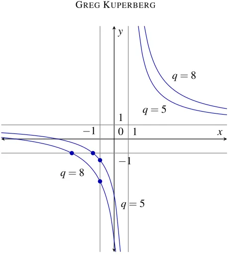
q=8
Figure 1: The Tutte plane with level curves ofq.
Proof. Figure 1shows a diagram of curves in thex-yplane (the Tutte plane) with constant values ofq. Given thatq>4 andx,y<0, we must have either thatx<−1 ory<−1 or both. Parallel composition has the same effect onyas series composition has onx, and vice versa; so we can assume without loss of generality thatx<−1. As a first step, we can create the dual weightxnwith a series composition withn edges. This creates a sequence of weightsynthat satisfies the estimate
log(yn) =qx−n(1+o(1))
asn→∞. Now suppose thaty0>1 is some other weight. We claim that we can efficiently approximate
y0as a product of weightsy2n. Equivalently, we claim that we can efficiently approximate log(y0)as a sum of terms log(y2n):
log(y0) =log(y2n1) +log(y2n2) +· · ·.
This can be viewed as a bin packing problem, because both log(y0)and each term log(y2n)are positive. The claim is established by using a greedy bin-packing algorithm. I. e., choose each term log(y2nk)to be as large as possible, but so that the partial sum does not exceed log(y0). Since the terms log(y2n)decrease exponentially (and no faster), and since the graph complexity of each term is linear inn, the result is a parallel-series composition which is anFPTEASfor the weighty0.
value other thany0=0. Since we also want the remaining weighty0=0, we can at this point achieve its dual weightx0=1−qwith a series composition with the dual weightsx0=−1 andx0=q−1.
4.4 Densely generatingPSL(W(n)P)
In this section, we will prove that ifq>4, then there areFPTEASnumbersx,y1, andy2, such that the gatesS(x),P(y1), andP(y2)and their inverses densely generate the group PSL(W(n)P)for anyn≥2.
Lemma 4.3says that we can obtain any such gates inFPTEASapproximation using subgraph gadgets. Our argument borrows from the author’s previous work [28] and makes crucial use of the Zariski topology on the group PSL(W(n)P).
TheZariski topologyon an algebraic group (or any algebraic variety) is by definition the topology in which the closed sets are solutions to polynomial equations. The Zariski topology onRnor on PSL(n,R) is much coarser than the standard topology, which in this context is called theanalytic topology. It is easier for a subgroup or a subset to be Zariski dense, and it is easier to prove Zariski denseness in this algebraically adapted topology. In particular:
Theorem 4.4 ([28, Cor. 1.2]). Let n>1 be an integer and let t >1 be real. Then the Jones braid
representation of B2nacting on W(2n)K=X(2n)Kwith parameter t is Zariski dense inPSL(X(2n)). On the other hand, in some circumstances we can get the best of both worlds:
Proposition 4.5([28, §3]). A subgroupΓof a connected, simple Lie group G is analytically dense if and
only if it is both analytically indiscrete and Zariski dense.
(Proposition 4.5is a baby version of a more famous result known as the Zassenhaus neighborhood theorem [39,22].)
To finish the construction, letq=t+2+t−1, letx=y1=−tandy2=t
√
2. (The the only requirement
is thaty2should be an irrational power oftwith anFPTEASexponent.) Then the gatesP(y1)andP(y2)
generate an indiscrete group by (4.4); their products
P(−t)aP(t
√
2)b
=P((−1)ata+
√
2b
)
for alla,b∈Z are a dense subset of allP(y). ByTheorem 4.2, the gates S(x) andP(y1)acting on W(n)P=W(2n)K generate the Jones braid representation ofB2n. ByTheorem 4.4, this group action is Zariski dense. With the addition of the gateP(y2), it is also indiscrete and therefore analytically dense by
Proposition 4.5.
Remark 4.6. A self-contained proof of Theorem 1.3 would be simpler if we applied some of the
techniques involved inTheorem 4.4directly to the group generated by gates of the formP(y)andS(x). However, these techniques involve yet another set of mathematical tools that we prefer to relegate to [28].
4.5 Proof ofTheorem 1.3
Proof. FollowingCorollary 3.2and its proof, let