Departamento de Ciências de Computação São Carlos – SP – Brazil
1[email protected],2[email protected]
Abstract. Process scheduling problems present a large solution space, which exponentially increases according to the number of computers and processes. In this context, exact approaches are, therefore, infeasible. This limitation motivated several works to consider meta-heuristics to optimize the search for good solutions. In that sense, this work proposes a new approach based on the Tabu Search to improve process scheduling by considering application knowledge and the logical partitioning of distributed en-vironments. Such knowledge comprises historical application events (captured during execution) which allow a better parametrization of the optimizer and, consequently, generates better results. Simulation results confirm the contributions of this new approach, which outperforms other techniques when dealing with large and heterogeneous environments, such as Grids.
Keywords:Process scheduling, Meta-heuristics, Tabu Search, Grid computing, Cluster computing.
(Received November 30, 2009 / Accepted September 15, 2010)
1 Introduction
Application-specific knowledge (for example: process-ing time, memory usage and communication) has been applied to improve process scheduling decisions [14, 22, 9, 20]. Such knowledge is obtained from the de-scription of the computational requirements provided by users, traces of all applications in production envi-ronments, or the specific monitoring of single applica-tions. The traces of all applications and specific mon-itoring have been confirmed to be efficient information sources [19]. Several techniques employ such knowl-edge to predict parallel application operations as a way to improve scheduling decisions [14, 22, 9, 20, 18, 4, 19].
Feitelson and Rudolph [9] conducted experiments making repeated application executions and observing their resources occupation. They observed that re-source consumption presents low variation when exe-cuting the same application and, therefore, concluded
that resource consumption can be estimated from his-torical information what avoids the explicit user coop-eration in parametrizing scheduling policies.
Harchol-Balter and Downey [14] studied how pro-cess lifetime (also called execution time or response time) can be used to improve scheduling decisions. They evaluated execution traces in a workstation-based environment and modeled probability distribution func-tions to characterize sequential application lifetimes. Based on those models, a load balancing algorithm was proposed, which employs such model to decide on pro-cess migrations. Mello et al. [5] extended that work by evaluating the processor consumption, what has im-proved the previous approach.
Pineau et al. [17] studied and presented limita-tions of deterministic scheduling algorithms on hetero-geneous environments. They concluded that scheduling optimization approaches highly depend on certain pa-rameters of such environments.
scheduling, however, with the advent of the Grid com-puting, new techniques have been proposed to ad-dress scheduling decisions by considering heterogene-ity and large scale environments. Yarkhan and Don-garra [24] compare a Simulated Annealing (SA) ap-proach to greedy search on a grid computing scenario. They concluded that SA improves scheduling results, due to it helps to avoid local minima. One of the draw-backs of that work is that the authors only consider one parallel application, this is, nothing else is evaluated under the same circumstances. Besides that, the study consider no historical information of applications.
On the other hand, Abrahamet al.[1] predicted pro-cess execution times and proposed nature-inspired heu-ristics, such as SA and Genetic Algorithms, to schedule applications on grids. Authors only consider Bag-of-Tasks1 applications, consequently, they do not model communication nor its impact on networks and schedu-ling.
Besides there are many grid-oriented approaches, most of them only address Bag-of-Tasks applications and, consequently, do not approach inter-process com-munication. Motivated by this limitation and by the pre-vious good results considering application knowledge [14, 22, 9, 20, 18, 4, 19], this work proposes a new approach to optimize process scheduling in heteroge-neous and large scale distributed environments based on the Tabu Search. This approach employs application knowledge (resource occupation), environment capaci-ties (processing, memory, hard disk and network) and current workloads as a way to reduce the total applica-tion execuapplica-tion time.
This approach considers a new network logical par-titioning technique, which groups the whole computing environment according to network latencies. This log-ical approach is conducted by a Tabu Search approach, which does not depend on physical partitioning nor en-vironment configurations. Processes are distributed on those computer groups (or logical partitions), what re-duces communication costs. Besides that, the cost in-volved in optimizing scheduling decisions has moti-vated the proposal of a new fitness function with time complexity ofO .
This paper is organized as follows: the process sche-duling problem is presented in Section 2; Section 3 de-scribes related optimization approaches; Section 4 pre-sents the Tabu Search and how it is employed in this work; Simulation results and comparisons to other tech-niques are presented in Section 5; Result analysis and contributions are described under Section 6.
1Bag-of-Tasks – this refers to independent tasks with no commu-nication among each other.
2 The Problem
In this paper, the scheduling problem consists in the dis-tribution of processes over a set of interconnected com-puters in order to reduce the application response time (also called execution time). The response time is the sum of the time consumed in processing, memory and network operations.
According to the formalization by Garey and John-son [11], we characterize the distributed scheduling problem optimization as follows. Let A be the set of parallel applications A {a0, a1, . . . , ak−1} and
size . the function which defines the number of pro-cesses that compose an application. Thus, each one of thekapplications is composed of a different number of processes, for example, size a0 ,size a1 etc. Consider, then, that the setPcontains all processes of allkparallel applications. In this way, the number of elements inP is equal to|P| �k−1
i=0 size ai .
Each processpj ∈P, wherej , , . . . ,|P| − ,
contains particular features, here named behavior, of resource utilization: CPU, memory, input and output. Consequently, every process requires different amounts of resources provided by the setV of computers of the distributed environment (where|V|defines the number of computers). Besides that, each computervw ∈ V,
wherew , , . . . ,|V| − , has different capacities in terms of CPU, main memory access latency, secondary memory read-and-write throughput, and network inter-face cards under certain features (bandwidth, latency and overhead to pack and unpack messages).
Computers in V are connected through different communication networks. All this environment can be modeled by a non-directed graphG V, E , where each vertex represents a computer vw ∈ V and the
communication channels in between vertices are edges {vw, vm} ∈ E. Those channels have associated
prop-erties such as bandwidth and latency.
The optimization problem consequently consists in scheduling the setP of processes over the graph ver-tices inG, attempting to minimize the overall execution time of applications inA. This time is characterized by the sum of all operation costs involved in process-ing, accessing memory, reading and writing on the hard disk, sending and receiving messages over/from the net-work.
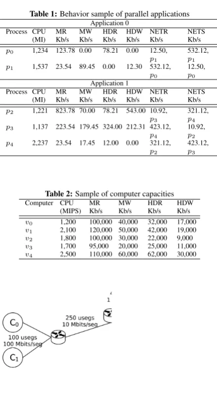
sec-ond from/to the hard disk – secsec-ondary memory; NETR and NETS are, respectively, the number of Kbytes re-ceived/sent per second from/over the network – in this situation, we also present the sender, for NETR, and the target process, for NETS).
Table 1:Behavior sample of parallel applications
Application 0 Process CPU
(MI) MRKb/s MWKb/s HDRKb/s HDWKb/s NETRKb/s NETSKb/s p0 1,234 123.78 0.00 78.21 0.00 12.50,
p1
532.12, p1
p1 1,537 23.54 89.45 0.00 12.30 532.12,
p0
12.50, p0
Application 1 Process CPU
(MI) MRKb/s MWKb/s HDRKb/s HDWKb/s NETRKb/s NETSKb/s p2 1,221 823.78 70.00 78.21 543.00 10.92,
p3
321.12, p4
p3 1,137 223.54 179.45 324.00 212.31 423.12,
p4
10.92, p2
p4 2,237 23.54 17.45 12.00 0.00 321.12,
p2
423.12, p3
Table 2:Sample of computer capacities
Computer CPU
(MIPS) MRKb/s MWKb/s HDRKb/s HDWKb/s v0 1,200 100,000 40,000 32,000 17,000
v1 2,100 120,000 50,000 42,000 19,000
v2 1,800 100,000 30,000 22,000 9,000
v3 1,700 95,000 20,000 25,000 11,000
v4 2,500 110,000 60,000 62,000 30,000
Figure 1:Example of network interconnection
Let the environment be composed of the five com-puters described in Table 2 (where MIPS represents the processing capacity in million of instructions per sec-ond; MR and MW are, respectively, the main mem-ory read-and-write throughput, in Kbytes per second; HDR and HDW are, respectively, the hard disk read-and-write throughput, in Kbytes per second – secondary memory). Such computers, inV, are interconnected according to Figure 1, which also presents the average network bandwidth and latency. Besides that, consider the scheduling operator defined by∝.
The distributed scheduling problem consists in defining on which computervw each process pj will
be placed on, considering the resource capacities and workloads. An example of solution for this instance is given byp0 ∝ v0, p1 ∝ v1,p2 ∝ v2,p3 ∝ v3 and
p4 ∝ v4. In this way, for each problem instance, we must schedule|P|processes on an environment com-posed of|V|computers, consequently, the universe of possible solutions is equal to|V||P|. For the previously presented instance, the problem has a solution universe equals to 5 , . Real problem instances can consider, for instance, , computers and applica-tions, containing processes each. In this situation, the solution space would be equal to , 64·512
, 32,768.
In this context, we may observe that the problem so-lution space is exponential and, therefore, we must pro-pose alternative approaches capable of providing good solutions in acceptable computational time. There is no polynomial-time algorithm to optimally solve this prob-lem (this is, to find the best solution at all), what allows to characterize it as intractable [11]. Given this fact, we may adopt algorithms that explore part of the solution space and find, by using guess and checking, a good candidate in non-deterministic polynomial time [11].
After characterizing the problem as intractable, it is important to understand how hard it is. In order to understand it, consider the equivalent NP-complete problem approached by Lageweg and Lenstra [16], and presented by Garey and Johnson [11]. This problem defines the process scheduling over m processors as follows:
Instance: Let the set of tasksT, a numberm∈Z+of processors, for each taskt∈Ta lengthl t ∈Z+and a weightw t ∈Z+, and a positive integerK.
Question: Is there a scheduling σ over m proces-sors for T, where the sum, for every t ∈ T, of
σ t l t ·w t is not higher thanK?
Such cost has motivated the adoption of meta-heuristics which are capable of finding approximate so-lutions in polynomial time.
3 Optimization Techniques
As previously presented, meta-heuristics have been considered for optimization purposes, due to their abil-ity to find good solutions in polynomial time. This sec-tion presents commonly considered meta-heuristics.
3.1 Genetic Algorithm
Genetic Algorithm [13] is an heuristic inspired in an-imal and plant evolution. It simulates the natural se-lection and genetic (characteristics) recombination as a way to explore diversity and, therefore, find solutions. Given a certain problem, solutions (codified as chro-mosomes) are described in terms of their characteristics (genes). Those chromosomes assume the role of indi-viduals in a population, where each one covers part of the solution space. Candidate solutions are evaluated using a fitness function which measures the optimiza-tion quality, considering specific problem constraints.
The algorithm periodically considers two genetic adaptations (operators), which change the chromosome characteristics and, consequently, better explores the search space. The considered operators are the mutation and crossover. Mutation randomly selects chromosome genes and changes their values. Crossover recombines chromosomes by considering the random exchange of genes, simulating the mating between living beings. Af-ter such adaptations, the modified chromosomes com-pose new candidate solutions to be evaluated. Popula-tions of candidates are assessed until converging to an acceptable quality or according to other constraints (e.g. time).
3.2 Hopfield Artificial Neural Network
The Hopfield artificial neural network [15] was intro-duced as an associative memory between input and out-put data. This network associates inout-puts and outout-puts using a Lyapunov energy-based function. This function is applied in dynamical systems theory in order to eval-uate stable states. The goal of such systems is to prove that modifications in the system state reduce the energy function results.
The use of an energy function has motivated the adoption of the Hopfield network to solve optimization problems. In that sense, the problem solution attempts to obtain the global minimum of the energy function, which represents the best solution for a certain instance. The connection weights of Hopfield network neurons
represent the energy function surface, which is explored to find minima regions.
The output function considered for Hopfield net-works [10] is defined in Equation 1, whereγis the con-stant gain parameter anduiis the network input for the
neuroni.
vi gi γui tanh γui (1)
In order to approach an optimization problem us-ing the Hopfield network, an energy function has to be defined and applied on the matrix that represents the system solution. This function defines constraints to acceptable solutions. The Hopfield artificial neural net-work applies the energy function on a possible solution, evaluates it and decreases the input values of neurons. Afterwards, it proposes a new solution to be analyzed. This cycle is executed until finding a solution that satis-fies all constraints.
3.3 Asynchronous Boltzmann Machine
The Asynchronous Boltzmann Machine is a general-ization of the Hopfield Neural Network which adds a stochastic element. While Hopfield considers thresh-olds to decide whether a neuron is activated, the Boltz-mann machine employs a probability function, de-scribed by neuron connection weights and threshold pa-rameters, as shown in Equations 2 and 3.
Ei
�
j
siwij−θi (2)
p i
e−ΔEi/T (3) The parameterT represents the temperature of the system. This concept is based on the increase and de-crease of temperature in real systems. We observe that high values ofT increase the probability of neuron ac-tivations, what allows fast convergence, however, it is likely to reach a local minima. Lower values are bet-ter when looking for a global minimum, although they consume more processing time.
The application of this technique is similar to Hop-field. The solution and the optimization function are similarly described. The temperature is gradually de-creased down to a limit when an output is issued. This technique presents a smaller bias toward local minima when compared to Hopfield networks.
3.4 Tabu Search
for good solutions. It applies the concept of movement and the Tabu list. In order to illustrate it, consider an op-timization problem where there is a finite setSwhich contains all possible (feasible or infeasible) solutions. Lets ∈ S be a solution andM s, parmovement be a
function overswith a set of parametersparmovement.
M . is called a movement ifM s, parmovement s�
wheres� ∈ S. This is, if it is possible to move from a solutionsto another ones�.
The set of parameters parmovement restricts the
movementM from a solution s to a limited number nof new solutions. Therefore,M . defines a subset inSwith sizenwhich is also called the neighborhood ofs, defined as n s. We may observe that solutions reached after a movement may or may not be feasible. The feasibility and quality of solutions are evaluated by a fitness function. Some works add constraints in the movement functionM . , consequently, only feasible solutions are accepted, what reduces the complexity of fitness functions.
The main idea of the Tabu Search is to navigate from a certain solutionsto somes� ∈n s , where, ideally,
s� presents a better quality. An usual implementation is to choose the best solution from n s, or a subset n� s ⊂ n s . It is important that the movement al-lows any solution to be reached from any other within a finite number of movements, otherwise the meta-heuristic does not cover all possible areas in the search space and potentially optimal solutions may never be visited.
In Tabu Search, there is a list of constraints indi-cating prohibited movements and parameters. Certain movements, or their parameters, are inserted in this list for a number of iterations, meanwhile, they are forbid-den and, consequently, avoided by the search algorithm. Once the movement function is defined and the Tabu criteria determined, the algorithm starts by choosing a random candidate solution and executing the function M . over it, usingmparameters inparmovement.
Im-plementations usually consider somem < k, wherekis the number of possible parameters to define the move-ment. The application ofM . over a candidate solu-tions, using each one of the mparameters, defines a subset of neighbor solutionsn s . The fittest solution found in neighborhood and its parameters are tabued for a certain number of iterations (i.e. they will not be used for a while). These steps are repeated until a stop criterion is reached, and the best solution visited is cho-sen. When tabuing a solution, the algorithm attempts to find other better candidates, this is, it better explores the search space.
3.5 Simulated Annealing
Simulated Annealing (SA) is an approach based on the metallurgic process of annealing, which consists of the successive heating and cooling of metals [2, 10]. Ac-cording to that process, the energy of atoms is contin-uously increased and decreased, leading to an equilib-rium state. SA simulates this process, looking for candi-date solutions in a state of high energy, or temperature, which is gradually reduced.
Similarly to the Tabu Search (Section 3.4) the con-cept of movement and neighborhood are considered. Once the best solution of the neighborhood,s�, is found, the algorithm probabilistically moves towards it using a probability function in the formP s, s�, T . Pis com-monly some function that has a bias in the direction of the best solution, eithersors�. The algorithm allows more random movements when the system energy (pa-rameterT) is high, but increases the bias towards good solutions when the energy is low, trying to escape from local minima. While these iterations are repeated, the temperature T is continuously decreased, until reach-ing a lower limit and findreach-ing a good solution.
3.6 Ant Colony Optimization
Ant Colony Optimization (ACO) is an optimization technique inspired in the behavior of ants in colonies [8]. When searching for food, ants wander randomly while laying down pheromone. Once the food is found, the ant returns home, reinforcing a pheromone path. Ants are attracted by pheromone and tend to priori-tize paths with such substance. The more intense the amount of pheromone in a path, the more likely other ants will follow it. After some time, the food paths will tend to be more intensively used and, therefore, have more pheromone. As several food paths may be found, the shortest one will be covered faster and, con-sequently, it will have more pheromone over it. After some time, there is a high probability to consider only the shortest path. ACO, similarly, attempts to find opti-mal paths while visiting neighbor solutions. The tech-nique considers virtual ants and pheromone to simulate the whole process.
4 Proposed Scheduling Approach
this work considers the Tabu Search technique, parame-trized with application knowledge, to find good schedu-ling solutions.
In order to employ knowledge, we developed online monitors to intercept application operations and store them on an experience database. In that sense, we con-sidered the knowledge acquisition model proposed by Sengeret al. [19], which supports the estimation of the expected behavior of new applications. This model looks for similar applications in execution traces, using a machine learning algorithm inspired in the Instance-Based Learning paradigm [3]. Execution traces of par-allel applications are considered as experience database and parallel applications are submitted to the system, as query points. The database information is, therefore, used by the learning algorithm to estimate the behav-ior of parallel applications (the behavbehav-ior includes esti-matives of the CPU, main and secondary memory, and network usages).
After employing the knowledge acquisition model, we consider the following application behavior com-ponents to parametrize our optimization approach: the processing consumption in million of instructions (MI), the total expected memory usage, and the network load, in terms of the number of messages per second and size (bytes). Then, such behavior components are used in our two Tabu-based optimization stages: 1) Firstly, the distributed environment is logically divided into smaller partitions, according to a first Tabu-based optimization approach. This approach considers the average inter-computer communication costs. This step reduces the full search space to local spaces, what makes the sec-ond stage of our approach run faster (consequently, it is more useful in real-world circumstances); 2) Sec-ondly, the incoming applications are distributed on one of the logical environment partitions (this logical par-tition does not require any configuration nor physical segmentation). In that sense, when an application ar-rives at the system, the logical partition with the low-est processing load is selected, and it executes another Tabu-based optimization approach to locally schedule application processes. Both stages are detailed next.
4.1 First Stage: A Tabu-Based Approach for Dis-tributed Environment Partitioning
Considering an environment composed ofV comput-ers, we intend to schedule applications on a subsetV� of it (whereV�⊂V), attempting to reduce communica-tion costs, and therefore the execucommunica-tion time, for all pro-cesses. In order to prevent high synchronization delays, we proposed a first stage of environment partitioning using a Tabu-based optimization approach. By
parti-tioning, this approach reduces the search space, this is, the number of candidate solutions for the second stage (Tabu-based approach for process scheduling), reduc-ing the time consumed to find good solutions.
In this stage, candidate solutions are represented by a set of computers. The movement function considers the swapping of a single computer from a logical par-tition to another. The fitness is computed by summing the communication costs in between every pair of com-puters in the same logical partition. The lower is the communication cost among computers in the same par-tition, the higher the solution quality is. The Tabu list is implemented by forbidding the last used movement for a number of iterations.
Our algorithm builds the initial solution dividing the whole environment into several logical partitions, con-taining at most z computers each (for evaluation pur-poses, our experiments consideredz ). The al-gorithm buildsnrandom parameters for the movement function, which are executed for the current solution. The resulting solutions are sorted and the best one is considered. As long as the correspondent movement is not in the Tabu list, the solution is selected, otherwise the next is chosen. These steps are repeated until the associated movement is not in the Tabu list, or every solution is examined. Thus, the selected solution be-comes the current one. The algorithm is iteratively re-peated until the best solution found is not modified for kiterations.
The size ofz is set by the administrator. Depend-ing on its value, this first Tabu-based stage divides the environment into smaller or larger logical partitions to received applications. A lowzreduces the search space for the second stage, however small partitions may have low computing capacity to fulfill the needs of certain applications. For example,z would create as many logical partitions as the number of computers in the en-vironment, then complete applications (including their processes) would be scheduled on the idler logical net-work, what, in this situation, is a single node. Oth-erwise, a very highz would join far away (far mean-ing high latency and low bandwidth) computers in the same logical partition, then, two communicating pro-cesses allocated on different and far computers would present high communication delays and, consequently, the performance would decrease.
4.2 Second Stage: Tabu Search for Process Distri-bution
receive new launched applications. Consequently, ap-plication processes are scheduled over nodes in that logical partition. This intra-partition scheduling is also based on a Tabu Search approach as presented next.
4.2.1 Description of the Solution
In this second stage we also consider the Tabu Search approach, in that sense we described candidate solu-tions using a matrix of computers (rows) versus pro-cesses (columns) – we may observe that one may choose to represent solutions using other data structures such as vectors, trees, etc. In our case, we use a sparse matrix which contains ’s and ’s, where a in column i and rowj represents processpi scheduled on
com-putervj ∈ V. The value depicts that the underlying
process is not located at the respective computer. In this context, we consider a feasible or valid solution when every process is scheduled on only one computer.
As an example consider an environment with com-puters. An application, containing processes, has to be distributed over this logical partition. A matrix is created containing a possible solution such as the one presented in Table 3. In this solution, each process is assigned to only one computer.
Table 3:Matrix of computers (rows) versus processes (columns) p0 p1 p2 p3
v0 0 0 1 0
v1 1 0 0 0
v2 0 0 0 0
v3 0 0 0 0
v4 0 1 0 0
v5 0 0 0 0
v6 0 0 0 1
4.2.2 Movement
In this second stage, the movement considers the swap of a processpi to another computer. This swap is
pa-rametrized by a number n, which defines how many changes are executed to the processpi over the sparse
matrix. In that sense, the movement function is repre-sented asM pi, n .
As an example, consider the solution described in Table 3. Let a movement be executed over it, where M p2, n , consequently, the process number or
p2, currently assigned tov0, will be changed in the ma-trix. An example of result is shown in Table 4. Nowp2 will be allocated on computerv4. This movement was
chosen since it never leaves the feasibly region of so-lutions and it can also reach any solution from this last (given an enough number of movements).
Table 4:Computers and Processes, Movement ofp2withn= 1
p0 p1 p2 p3
v0 0 0 0 0
v1 1 0 0 0
v2 0 0 0 0
v3 0 0 0 0
v4 0 1 1 0
v5 0 0 0 0
v6 0 0 0 1
4.2.3 Tabu List
In this second stage, we defined a Tabu List over the pa-rameters of the movement functionM pi, n , wherepi
is the process that will be transferred to another com-puter, and n is the number of swaps. This Tabu list works as follows: after executing a movement overpi,
givenn, that action (or movement itself) is added into the Tabu list and, consequently, forbidden for a number of algorithm iterations.
4.2.4 Fitness Function
As described in Section 3.4, the Tabu Search algorithm requires a fitness function, which evaluates the quality of a solution. The fitness is the target function to be minimized. As proposed, the parameters of this func-tion are based on the applicafunc-tion-specific knowledge, which includes the total processing cost, memory and network usage. We also consider knowledge about the environment, such as the current workload of comput-ers as well as their capacities and network overheads.
The purpose of our function is to estimate the total computer workload when considering a new candidate solution. This estimative is made by computing the total time consumed when processing instructions, the pro-cessing slowdown caused by memory usage (main and virtual memory usage), and the inter-process communi-cation cost.
execution, which also calculated the slowdown caused by memory usage (when a process consumes memory, processing time is penalized. Mello and Senger [6] con-cluded that the more the main and virtual memories are occupied, the higher is the slowdown in process execu-tion), as presented in Algorithm 1, whereT vj is the
memory slowdown function of computervj, proposed
by Mello and Senger [6], defined in Equation 4 (where vmjis the main memory size,vsj the virtual memory
size andxis the total memory currently used in compu-tervj– all of them in megabytes).
The parameters forT vj were defined according to
an average of experiments executed on heteroge-neous computers which (conducted in our laboratory) [6]. Among the evaluated computers, we had: AMD 2600+, AMD 64 bits and Intel Pentium 4 and Intel Core 2 Duo processors.
Therefore, function T vj generates a slowdown
factor to be multiplied by the processing time con-sumed. This factor models delays when processes are accessing main and virtual memories. The slowdown is a function of the memory being currently used (x, in Megabytes, in Equation 4). If only the main memory is being used and no swap is done, the slowdown grows linearly according to the amount of megabytes in mem-ory. When swap starts to be used, the slowdown causes an exponential influence in the process execution.
T(vj) =
8 > > > > > <
> > > > > :
1 when using less than 0.089
0.0069Megabytes
0.0068×x−0.089 when using more than
0.089
0.0069Megabytes and less thanvmjMegabytes
1.1273×exp((vmj+vsj)×0.0045) otherwise (4) The Algorithm 1 adds up all the slowdown caused my memory usage and the expected processing time. This fitness function was, then considered to make op-timizations. However, we observed that its time com-plexity was too high and simulations took long to exe-cute. Then, we started studying other approaches and end up proposing a polynomial equivalent version of this first. Such approach is presented as follows.
LetEi be the expected execution time for a single
processpi. LetDi andIi be respectively the decimal
and integer part ofEi, thereforeEi Di Ii. Let|Q|
be total the number of processes currently in the pro-cessor queueQ. Assume that the queue is kept ordered by the expected processing time (i.e. the process with the lowest expected time is executed first and so on).
Now consider a queue or circular list where pro-cesses were previously scheduled. Assume that ev-ery process can reside in the CPU for at most sec-ond, which is usually referred as CPU quantum (or
Algorithm 1Process Time and Memory Simulation
1: DefinesimulationT ime= 0.0
2: DefinetotalT ime= 0.0
3: DefinetotalM emory= 0.0
4: Define the expected memory usage for a computer (i.e. the sum of the expected memory usage for all processes)
ascomputerM emory
5: Define the vector (or queue) which contains running pro-cesses asrunningP rocess[]
6: whilerunningP rocessis not emptydo 7: forevery processpinrunningP rocessdo
8: totalM emory+= T(computerM emory)
9: ifp.expectedT ime< 1then
10: simulationT ime+=p.expectedT ime
11: totalT ime+=simulationT ime
12: removepfromrunningP rocess
13: computerM emory-=p.memory
14: else
15: simulationT ime+=1
16: p.expectedT ime-=1
17: end if 18: end for 19: end while
20: return [totalT ime,totalM emory]
time slice) [23]. Consider a set ofnprocesses in such queue. Now, let a processpineedIi.Diseconds to
fin-ish, whereIiis the integer andDithe decimal part,
re-spectively. This queue is sorted according toIj.Dj ∀j,
thus, a process at an indexj will finish before j . However, we consider a Round-Robin local scheduling policy (by local we mean the CPU policy and not the distributed environment policy), which will schedule p0, p1, . . . , pj−1, in such order, beforepj. In that sense,
there is some probability thatpj−1finishes before us-ing all the CPU quantum and the scheduler releases the CPU and gives it to the next process, this ispj.
Let Ei be an estimative of the expected execution
time for the processpiin such queue where other
pro-cesses were also added, whereiis the queue index. We observe that the total execution time of each process is always greater than or equal to the time of the previ-ous one (since the queue is kept sorted according to the expected execution times). Since the maximum time a processpi can reside in the CPU is , its integer
ex-pected timeIidetermines how many times it will enter
and leave the queue, and the decimal part determines the remaining time to finish execution. When all pre-vious processes have finished executing and since there are|Q| −i− remaining processes afterpi(which have
larger or equal processing time), the total time thatpi
cir-cle in the queue – this happens due to we consider the Round-Robin policy as the local CPU scheduler).
Now consider that every process has already exe-cutedIi−1times (this is, the total integer part ofpi−1), then processpi returns to the processor onlyIi−Ii−1 times. So, the remaining time of processpi, after all
previous processespj ∀j < i have finished, is given
by Ii −Ii−1 × |Q| −i , plus Di. Hence the
to-tal execution time for any process, considering only the processing time of its instructions is given by the total time currently executed increased by its own remaining time, according to Equation 5.
Ei Ei−1 Di Ii−Ii−1 × |Q| −i (5)
Therefore, the total expected processing time for a computer is given by Equation 6, assumingE−1 .
n
�
i=0
Ei−1 Di Ii−Ii−1 × |Q| −i (6)
Equivalently, the memory terms may be obtained as follows. Letmjbe the total memory of each processpj
andMibe the sum of all memory allocated at the
com-puter, in the moment that processpifinishes executing.
The total impact of the memory in a computer is the sum of all the occupied memory. Hence, every time a process is at the processor, its overall time is impacted by the slowdown factor (computed according the main and virtual memory usage), as shown by Mello and Sen-ger [6]. Consequently, the factor represents the slow-down impact being applied until the moment the pro-cesspileaves the queue, thusMi Mi−1−mi−1. To allow a proper mathematical model, letM−1 M0
M whereM is the total sum of memory beforehand, andm−1 . Assume that the impact of the mem-ory on a process when it remains less than one second (t < ) at the processor is equivalent to the impact caused by the remaining one second. Analog to the pro-cessing time, we can defineTias shown in Equation 7,
whereT vj Mi is the slowdown impact caused by
the memory currently used in computervj, after
finish-ing all processespj∀j < i. The total memory is given
by Equation 8.
Ti T vj Mi × Ii−Ii−1 × |Q| −i (7)
n
�
i=0
T vj Mi × Ii−Ii−1 × |Q| −i (8)
The two previously presented equations can be map-ped to an incrementally polynomial time complexity al-gorithm (as presented in Alal-gorithm 2).
Algorithm 2Process Time and Memory Simulation
1: DefinetotalT ime= 0.0
2: DefinetotalM emory= 0.0
3: Define the expected memory usage for a computer (i.e. the sum of the expected memory usage for all processes)
ascomputerM emory
4: Define the vector (or queue) which contains running pro-cesses asrunningP rocess[]
5: DefinelastInteger= 0
6: forevery processpinrunningP rocessdo 7: Definep.expectedT imeinteger part asI
8: Definep.expectedT imedecimal part asD
9: Definepindex on the array asi
10: totalM emory += T(computerM emory) * ((I
-lastInteger) * (runningP rocess.size-i) +1)
11: totalT ime += D + (I - lastInteger) *
(runningP rocess.size-i)
12: lastInteger=I
13: end for
14: return [totalT ime,totalM emory]
Further improvements were made to create a fitness function of time complexityO . Using Equation 6, an attempt was made in order to find the difference be-tween the expected processing time before and after in-serting a new process. Equation 5 represents the total execution time associated to a certain process in the sys-tem. Let a processpk, with processing timeIk Dk,
be inserted in the system at the queue indexj. LetEk
represent the estimated execution time of the inserted processpk, which impacts in the execution time of all
processes already in the queue. Therefore,Ekis defined
in Equation 9. After inserting a process at the queue in-dex j, the execution time of every process pi, which
was previously referred asEi, is now calledEi. This
new nomenclature makes evident that the expected exe-cution time has changed for every process. In Equation 10, the time associated to the processpkis presented.
Ek Ej−1 Dk Ik−Ij−1 × |Q| −j wherek j (9)
Equation 9 computes the expected execution time of processpk(Ek) by considering the estimated execution
Now that a new process has been inserted in the queue, the process pj, which was previously in index
j, moves to the positionj and its expected time now depends onEk. Equation 10 illustrates this (notice
that we still refer to this process aspj, even though its
index has changed).
Ej Ek Dj Ij−Ik ×
|Q| − j (10)
We now define the remaininghatEi, for alli < k
andi > k, wherekis the index where processpk was
inserted (k j). For processespi ∀ i < j, Equation
5 can be used to determine the expected times straight-forwardly. For processespi ∀ i > jthe multiplicative
factor n −i changes to n − i (re-member that we are comparing the processes expected times in the initial setup with the ones after the inser-tion, therefore i is an index from the initial position, and becomesi ∀i > jin the final setup). This is demonstrated in Equation 11.
Ei
¯ ˆ
Ei−1+Di
+(Ii−Ii−1)×((n+ 1)−i) i < j
¯ ˆ
Ei−1+Di
+(Ii−Ii−1)×((n+ 1)−(i+ 1)) i > j
(11)
By maintaining the initial indices i, it is possible to calculate the difference of the expected times for each processpi before and after the insertion of
pro-cesspk. Using Equations 9, 10 and 11, we calculate
Ei−Ei ∀ pi, whereEi is the estimated time for the
processpibefore the insertion ofpk. The result is
pre-sented in Equation 12.
Ei−Ei
(Ii−Ii−1) + ((Ii−1−Ii−2) +. . .+ (I0−I
−1) i < j
¯ ˆ
Ei+Di+Pj−
1
a=0(Ia−Ia−1) +Dk+Ik−Ij−1 i≥j
(12)
These differences can be written in the form of sums, as presented in Equations 13 and 14.
j−1
�
i=0
Ei j−1
�
a=0 a
�
b=0
Ib−Ib−1 (13)
Pn−1
i=j
¯ ˆ Ei=
(|Q| −j)×(Pj−1
a=0(Ia−Ia−1) +Dk+Ik−Ij−1)
(14)
Such equations represent the time to be added to the total execution time of each processpi, initially in the
queue, after the insertion of processpk at the position
j. If these sums are added toEk(the expected time for
pk), the total difference between the current expected
time and the time after the insertion is found (obviously the time ofpk must be considered integrally in the
dif-ference, sincepkwas not in the queue beforehand). So,
the total difference is defined in Equation 15, whereIi
andDiare the integer and decimal times expected for
eachpi in the original queue (i.e. all the sums iterate
over the initial queue, not the one afterpk is inserted,
thusiranges from to|Q| − ), and|Q|is the number of processes initially at the queue.
Ek
|Q|−1
�
i=0
Ei |Q|
j−1
�
i=0
Ii−Ii−1 − j−1
�
i=0
Di Ik |Q| −j
|Q| −j Ij−1 Dk Ik (15)
All the sums considered by the equations only de-pend on the current values. This behavior allows these sums to be incrementally computed every time the al-gorithm is executed. Then, in order to evaluate new so-lutions, we consider the current computer status, thus, taking advantage of previous computations and, there-fore, making the algorithm faster.
The calculation of the memory considers the same procedure. Let Ti be the associated memory
calcula-tion, which represents the total memory impact for pro-cesspiafter the insertion of processpk, andMibe the
new total memory associated to every process after the insertion. Again the new processpk is inserted at the
positionj. The correspondentTiis defined in Equation
16. Wheni < j,Mi Mi mk, sinceM0 �nmi.
Fori≥j,Mi MisinceMi Mi−1−mi−1.
T mi
T(Mi+mk)×(Ii−Ii−1)(|Q| −i+ 1) i < j
T(Mi)×(Ii−Ii−1)(|Q| −i+ 1) i > j
T(Mi)×(Ii−Ik)(|Q| −i+ 1) i=j (16)
It can be observed that for values between . and the total main memory, the function T . allows thatT a b T a T b . if both, aand b, are in this range. This fitness function assumes that every value for memory inside a functionT . is in this range in the following calculations.
T mi−T mi
T(Mi)(1 + (Ii−Ii−1))+
(T(mk) + 0.089)
(1 + (Ii−Ii−1)(|Q| −i+ 1)) i < j
T(Mi)(Ik−Ij−1)(|Q| −i) i=j
0 i > j
(17)
The sum of the differences andT mk are defined in
Equation 18.
n
�
i=0
T mi−T mi j−1
�
i=0
T Mi Ii−Ii−1
T Mj Ik−Ij−
T mk . j Ik |Q| −j j−1
�
i=0
Ii (18)
Since the sums are incrementally updated at every algorithm cycle, it allows aO complexity for the cal-culation.
4.2.5 Tabu Search Algorithm
The algorithm starts by creating a fully random solu-tion, since any solution will work, and setting it as the current solution. Iteratively, a certain numbermof ran-dom parameters for the movement are generated. For each one of the generated parameters, a movement is executed over the current solution. The resulting solu-tions are sorted out and the one with the best fitness is chosen (lowest execution time). If the movement that leads to it is in the Tabu list, the next solution is cho-sen, and so on, until a solution, which is not tabued, is found, or every solution is examined. The chosen solu-tion is set as the current solusolu-tion, and the correspondent movement is inserted in the Tabu list for a certain num-ber of iterations. At the end of the iteration, the current solution is compared to the best one found and replaces it when better.
The algorithm stops when a certain number of iter-ationskis elapsed and no improvements were made to the current solution.
5 Simulations
In order to validate our approach, several simulations were conducted using SchedSim, a multicomputer en-vironment simulator written by Melloet al. [6]. This simulator allows the execution and comparison of dif-ferent scheduling policies.
SchedSim was written in Java language, and has an interface,SchSlowMig, which allows the implemen-tation of scheduling algorithms. Once implemented, the simulator will request computers to each incoming process, hence allowing the scheduling policy to take place.
SchedSim use probability distribution functions to simulate the application arrival as well as its behavior. It is parametrized using the number of computers in the network and their characteristics, the number of appli-cations, processes per application and the network com-munication costs. It executes by generating applications according to probability distribution functions and issu-ing requests to the scheduler to distribute them. The simulation calculates all the time spent in CPU, mem-ory, hard disk and network operations, returning the av-erage application response time (or execution time) and the standard deviation. It also computes the time spent by the scheduling policy.
5.1 Parametrization
Simulations were conducted using the following envi-ronments: -node cluster and a -node grid, consid-ering application sizes (number of processes) of and processes. The number of applications ranged from to . The simulations considered inter-message intervals of around second (messages were gener-ated according to an exponential probability distribu-tion funcdistribu-tion with average of , million of tions per second – this considers the number of instruc-tions between consecutive message events). These mes-sages are sent and received through the network (by the processes of the application), characterizing inter-process communication.
Applications dynamically arrive at the environments after they start executing. The application allocation cannot be static, since multiple runs are necessary to acquire application specific parameters.
The capacity of every computing resource was gen-erated by using Normal probability distribution func-tions with the following averages:
1. Processing capacity – , MIPS (million of in-structions per second);
2. Main memory capacity – , MBytes;
3. Virtual memory – , MBytes;
area networks with one to five computers each (what tends to be closer to an opportunistic grid).
The cluster nodes were connected through a Gigabit Ethernet infrastructure with RTT (Round-Trip Time) of . second, obtained from a benchmark by Mello and Senger [6]. On the other hand, experiments were carried out to characterize the latency in between the grid nodes. Local, metropolitan and worldwide net-works were analyzed and, according to results, we de-fined an exponential probability distribution function (with average . second) to model the network latency behavior.
The Tabu-based logical network partitioning algo-rithm was implemented to group the environment nodes into smaller networks with at most computers. The parameterm, this is the total number of random move-ments per iteration, was set to . The number of total iterations to the stop criterionkwas set to . Afterk iterations, if no better solution is found, the algorithm stops. Simulations were executed in the SchedSim sim-ulator [6] comparing our Tabu Search approach to other scheduling policies.
5.2 Comparison to other Scheduling Policies The proposed Tabu Search approach was compared, by using simulations, to the following policies: Random [21], Route [7] and RouteGA [4]. They were evaluated under the same conditions. It is important to make clear that only the approach proposed here makes the logical partitioning. This partitioning does not physically mod-ify the environment (but just reduces the search space for feasible optimization solutions).
The Random algorithm randomly chooses a compu-ter to allocate every process. The Route technique, pro-posed by Mello and Senger [7], creates neighborhoods by choosing computers with low communication cost. When an application is launched on a certain compu-ter, it is distributed over its neighbors, considering the processing load and application runtime. The neighbor may redistribute processes according to the migration model proposed by Mello and Senger [5]. RouteGA is an extension of Route, which considers the meta-heuristic of Genetic Algorithms to select the best neigh-borhood to distribute processes.
5.3 Results
Results, in terms of the average execution time of ap-plications and confidence intervals of (in seconds), are presented in Tables 5, 6, 7 and 8. The numbers rep-resent the average response time and confidence inter-vals for every policy.
We observe that this instance of the Tabu Search, in most of the cases, presents better results than other techniques. The considerably better results in grids are consequence of the network logical partitioning, per-formed before the process scheduling. This partition-ing restricts the search space and improves the overall meta-heuristic performance (it plays the important role of defining a hierarchy for scheduling). In cluster envi-ronments, the results were only slightly better than the best available technique, which is RouteGA.
We also observe that the confidence interval was considerably wide for the grid computing environment. This happens to due there are few computers in every local area network (up to ) and the communication costs in between computers are high. This simulates the opportunistic-type of grid computing architecture. Besides that, applications have more processes than the number of computers per local area network, what tends to require computers in different networks and, there-fore, increases the execution time dispersion. On the other hand, by executing the network logical partition-ing, our Tabu Search approach considerably improves such confidence interval due to the allocation of pro-cesses in nearby regions (according the inter-computer communication costs). Such allocation, reduces the dis-persion of the execution time, ensuring higher perfor-mance to applications. Consequently, by using hierar-chical scheduling, we obtain application performance improvements.
Table 5:Results for Cluster with32computers and applications up
to32processes
# Apps Random Route RouteGA Tabu
10 3.2493± 2.4423± 1.9295± 2.1011± 0.1582 0.2502 0.0423 0.0319 20 20.195± 15.394± 8.2093± 7.5915±
0.2948 47.857 0.4221 0.1306 30 19.975± 15.042± 9.4902± 7.7338±
0.4704 40.685 1.0870 0.2707 40 13.565± 12.729± 9.5049± 7.7394±
0.1997 11.872 0.2350 0.0929 50 41.046± 20.865± 14.856± 12.064±
0.8057 18.095 1.1616 0.3185 60 45.616± 37.250± 22.024± 21.576±
2.2791 33.261 0.9666 0.9009 70 55.718± 42.751± 27.567± 24.397±
1.5792 42.725 0.7663 0.7997 80 53.241± 46.781± 29.107± 25.953±
1.7958 57.306 1.5444 2.5727 90 120.04± 113.19± 60.053± 58.722±
3.5824 44.081 4.5557 2.9846 100 172.61± 160.44± 85.808± 81.985±
4.9879 48.078 4.8041 4.1718
Table 6:Results for Cluster with32computers and applications up
to128processes
# Apps Random Route RouteGA Tabu
10 4.5429± 3.8921± 3.4337± 3.7729± 0.4759 0.2230 0.1812 0.2286 20 13.575± 12.463± 10.806± 10.069±
5.6920 2.9334 0.7079 0.9039 30 14.706± 13.025± 11.331± 10.119±
7.8257 7.7339 1.5323 0.8143 40 15.157± 15.009± 14.575± 11.516±
3.2099 7.6891 1.2135 0.6116 50 15.660± 14.345± 15.953± 12.337±
1.7992 0.4912 0.7219 0.3532 60 78.386± 69.323± 40.034± 42.242±
385.25 87.872 9.4197 10.772 70 81.029± 70.640± 50.024± 44.536±
351.45 40.463 4.6634 6.7419 80 83.091± 75.105± 51.633± 46.073±
238.78 91.058 11.584 16.828 90 328.59± 311.69± 172.09± 167.17±
568.13 138.08 31.060 33.258 100 544.14± 533.22± 292.48± 279.83±
2085.7 269.40 55.243 33.044
Table 7:Results for Grid with512computers and applications up to 32processes
# Apps Random Route RouteGA Tabu
10 95.906± 104.04± 19.668± 7.5879± 13208. 9734.7 111.25 5.1062 20 263.12± 332.69± 39.809± 20.128±
42801. 38046. 913.85 62.788 30 337.78± 299.05± 41.720± 21.288±
54501. 24436. 740.04 124.46 40 239.23± 236.32± 27.513± 15.434±
29344. 21958. 480.62 41.274 50 323.04± 291.93± 27.968± 19.308±
26934. 20039. 259.21 44.102 60 434.90± 636.46± 83.579± 53.369±
24922. 153632 961.32 299.19 70 617.47± 598.82± 178.80± 62.614±
399973 383541 59228. 546.76 80 988.35± 966.52± 488.94± 48.155±
167369 170541 125555 121.96 90 619.89± 551.21± 155.03± 69.901±
63420. 82274. 5075.9 435.07 100 558.69± 475.73± 148.71± 70.304±
134920 62375. 1082.6 76.408
and Round-Robin in most of the situations.
6 Conclusions
Motivated by the exponential complexity and meta-heuristics results, this paper proposes a new process scheduling approach using the Tabu Search. Results confirmed that the proposed approach presents better results than other techniques, considering different en-vironments. The approach also reasonably keeps low costs to compute the scheduling optimization, due to its efficientO fitness function, and the logical network partitioning performed beforehand.
In clusters with computers, the approach slightly outperforms other techniques. It does keep low costs, mostly because of the low complexity fitness function.
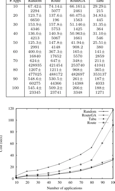
Table 8:Results for Grid with512computers and applications up to 128processes
# Apps Random Route RouteGA Tabu
10 67.42± 74.14± 66.161± 29.29±
2294 5077 2461 215
20 123.7± 137.6± 60.475± 34.83±
6650 196 1563 445
30 153.9± 157.8± 51.146± 31.35±
4346 5753 1425 364
40 136.0± 140.9± 50.963± 31.10±
4213 5067 1661 546
50 125.3± 147.8± 41.94± 25.51± 2991 4148 908.2 380 60 400.0± 367.3± 165± 141±
16840 17652 5570 2859
70 624± 647± 348± 211±
428935 421454 253740 41041
80 1207± 1211± 968± 365±
477025 488172 482697 353137 90 548.6± 530.5± 261± 187±
60275 44366 14388 4033 100 545.4± 509.2± 266± 188±
23345 23741 3348 1271
0 20 40 60 80 100 120
10 20 30 40 50 60 70 80 90 100
Cost (secs)
Number of applications Random RouteGA Tabu Route
Figure 2: Costs for the32-node Cluster with applications up to32
processes
0 200 400 600 800 1000 1200
10 20 30 40 50 60 70 80 90 100
Cost (secs)
Number of applications Random RouteGA Tabu Route
Figure 3:Costs for the32-node Cluster with applications up to128
processes
0 100 200 300 400 500 600 700
10 20 30 40 50 60 70 80 90 100
Cost (secs)
Number of applications Random RouteGA Tabu Route
Figure 4: Costs for the512-node Grid with applications up to32
processes
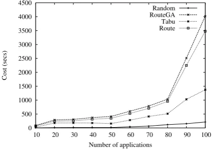
0 500 1000 1500 2000 2500 3000 3500 4000 4500
10 20 30 40 50 60 70 80 90 100
Cost (secs)
Number of applications Random RouteGA Tabu Route
Figure 5: Costs for the512-node Grid with applications up to128
processes
costs, due primarily to the logical partitioning of the network in the first stage of the algorithm. Those results show a general superior performance of Tabu Search in the considered environments.
The low costs observed in the simulations are a con-sequence of the flexibility of the stop criteria combined to a low strictness in the movement, and the low com-plexity fitness function adopted. The partitioning of the network environment also considerably reduces the search space (as observed in the section 2), therefore allowing the usage of the divide-and-conquer approach which is faster.
The tolerant stop criterion allows the algorithm to stop quickly, choosing a solution without an exact search. The reduced strictness diminishes the num-ber of evaluated candidate solutions what decreases the time consumed by the algorithm, at the expense of wast-ing potentially good solutions.
Results presented in Table 8 confirm that, for grids,
the Tabu Search presents better results, due to the en-vironment partitioning. Other techniques have been un-able to explore the search space so efficiently, as they do not employ such method. The exponentially larger un-partitioned search spaces are much harder to explore us-ing meta-heuristics, exponentially increasus-ing the costs to achieve high quality results. Furthermore, the logical partitioning also considerably reduced the confidence interval of execution time for grid environments, ensur-ing higher performance to applications. This confirms that by using hierarchical scheduling, we obtain appli-cation performance improvements.
References
[1] A. Abraham, R. B. and Nath, B. Nature’s heuristics for scheduling jobs on computational grids. In 8th IEEE International Conference on Advanced Computing and Communications (AD-COM 2000), India, 2000.
[2] Aarts, E. and Korst, J. Simulated annealing and Boltzmann machines: a stochastic approach to combinatorial optimization and neural comput-ing. John Wiley & Sons, Inc., New York, NY, USA, 1989.
[3] Aha, D. W., Kibler, D. F., and Albert, M. K. Instance-based learning algorithms. Machine Learning, 6:37–66, 1991.
[4] de Mello, R. F., Filho, J. A. A., Senger, L. J., and Yang, L. T. RouteGA: A Grid Load Balancing Algorithm with Genetic Support. In21st Interna-tional Conference on Advanced Networking and Applications, pages 885–892, Aug. 2007.
[5] de Mello, R. F. and Senger, L. J. A new migration model based on the evaluation of processes load and lifetime on heterogeneous computing environ-ments. InInternational Symposium on Computer Architecture and High Performance Computing -SBAC-PAD, page 6, 2004.
[6] de Mello, R. F. and Senger, L. J. Model for sim-ulation of heterogeneous high-performance com-puting environments. In7th International Confer-ence on High Performance Computing in Compu-tational Sciences – VECPAR 2006, page 11, 2006.
[8] Dorigo, M. and Stützle, T. Ant Colony Optimiza-tion. MIT Press, 2004.
[9] Feitelson and Nitzberg. Job characteristics of a production parallel scientific workload on the NASA ames iPSC/860. In Feitelson, D. G. and Rudolph, L., editors,Job Scheduling Strategies for Parallel Processing – IPPS’95 Workshop, volume 949, pages 337–360. Springer, 1995.
[10] Freeman, J. A. and Skapura, D. M. Neural net-works: algorithms, applications, and program-ming techniques. Addison Wesley Longman Pub-lishing Co., Inc., Redwood City, CA, USA, 1991.
[11] Garey, M. R. and Johnson, D. S. Computers and Intractability : A Guide to the Theory of NP-Completeness. Series of Books in the Mathemati-cal Sciences. W. H. Freeman, January 1979.
[12] Glover, F. and Laguna., M.Tabu Search. Kluwer, Norwell, MA, 1997.
[13] Goldberg, D. E. Genetic Algorithms in Search, Optimization and Machine Learning. Kluwer Academic Publishers, Boston, MA., 1989.
[14] Harchol-Balter, M. and Downey, A. B. Exploit-ing Process Lifetimes Distributions for Dynamic Load Balancing.ACM Transactions on Computer Systems, 15(3):253–285, August 1997.
[15] Hopfield, J. J. Neural networks and physical sys-tems with emergent collective computational abil-ities. Neurocomputing: foundations of research, pages 457–464, 1988.
[16] Lageweg, B. J. and Lenstra, J. K. Private commu-nication, 1977.
[17] Pineau, J.-F., Robert, Y., and Vivien, F. The im-pact of heterogeneity on master-slave scheduling. Parallel Comput., 34(3):158–176, 2008.
[18] Senger, L. J., de Mello, R. F., Santana, M. J., and Santana, R. H. C. An on-line approach for classi-fying and extracting application behavior on linux. InHigh Performance Computing: Paradigm and Infrastructure (to appear). John Wiley & Sons, 2005.
[19] Senger, L. J., Mello, R. F., Santana, M. J., and Santana, R. H. C. Aprendizado baseado em in-stâncias aplicado à predição de características de execução de aplicações paralelas. Revista de In-formática Teórica e Aplicada, 14:44–68, 2007.
[20] Senger, L. J., Mello, R. F., Santana, M. J., San-tana, R. H. C., and Yang, L. T. Improving schedu-ling decisions by using knowledge about parallel applications resource usage. InHigh Performance Computing and Communications: First Interna-tional Conference (HPCC), LNCS 3726, volume 3726, Sorrento, Itália, September 2005.
[21] Shivaratri, N. G., Krueger, P., and Singhal, M. Load distributing for locally distributed systems. IEEE Computer, 25(12):33–44, 1992.
[22] Silva, F. A. B. D. and Scherson, I. D. Improving Parallel Job Scheduling Using Runtime Measure-ments. In Feitelson, D. G. and Rudolph, L., ed-itors, Job Scheduling Strategies for Parallel Pro-cessing, pages 18–38. Springer, 2000. Lect. Notes Comput. Sci. vol. 1911.
[23] Tanenbaum, A. S. Modern Operating Systems. Prentice Hall, New Jersey, 1992.