www.theoryofcomputing.org
S
PECIAL ISSUE: APPROX-RANDOM 2015
Improved
NP
-Inapproximability for
2-Variable Linear Equations
Johan Håstad
∗Sangxia Huang
†Rajsekar Manokaran
‡Ryan O’Donnell
§John Wright
¶Received December 25, 2015; Revised October 25, 2016; Published December 24, 2017
Abstract: An instance of the 2-Lin(2) problem is a system of equations of the form “xi+xj=b (mod 2).” Given such a system in which it is possible to satisfy all but anε
fraction of the equations, we show it isNP-hard to satisfy all but aCε fraction of equations, for anyC<11/8=1.375 (and any 0<ε ≤1/8). The previous best result, standing for
over 15 years, had 5/4 in place of 11/8. Our result provides the best knownNP-hardness even for the Unique-Games problem, and it also holds for the special case of Max-Cut. The
A preliminary version of this paper appeared in the Proceedings of the 18th International Workshop on Approximation Algorithms for Combinatorial Optimization Problems (APPROX 2015) [16].
∗Supported by ERC Advanced Investigator Grant 226203 and the Swedish Research Council.
†Work done when the author was a doctoral student at KTH, Sweden. Supported by ERC Advanced Investigator Grant
226203, the Swedish Research Council, and ERC Starting Grant 335288.
‡Work done when the author was a post-doctoral researcher at KTH, Sweden. Work supported by ERC Advanced Investigator
Grant 226203.
§Department of Computer Science, Carnegie Mellon University. Supported by NSF grants CCF-0747250 and CCF-1116594
and a grant from the MSR–CMU Center for Computational Thinking.
¶Work done when the author was a graduate student at CMU. Work supported by NSF grants 0747250 and
CCF-1116594 and a grant from the MSR–CMU Center for Computational Thinking.
ACM Classification:F.1.3, F.2.2, G.1.6
AMS Classification:68Q17, 68W25
precise factor 11/8 is unlikely to be best possible; we also give a conjecture concerning analysis of Boolean functions which, if true, would yield a larger hardness factor of 3/2.
Our proof is by a modified gadget reduction from a pairwise-independent predicate. We also show an inherent limitation to this type of gadget reduction. In particular, any such reduction can never establish a hardness factorCgreater than 2.54. Previously, no such limitations on gadget reductions was known.
1
Introduction
The well-known constraint satisfaction problem (CSP) 2-Lin(q)is defined as follows: Given n vari-ablesx1, . . . ,xn, as well as a system of equations (constraints) of the form “xi−xj =b (modq)” for constantsb∈Zq, the task is to assign values fromZqto the variables so that there are as few unsatisfied constraints as possible. It is known [18, 20] that, from an approximability standpoint, this problem is equivalent to the notorious Unique-Games problem [17]. The special case of q=2 is particularly interesting and can be equivalently stated as follows: Given a “supply graph”Gand a “demand graph”H
over the same setV of vertices, partitionV into two parts so as to minimize the total number of cut supply edges and uncut demand edges. The further special case when the supply graphGis empty (i. e., every equation is of the formxi−xj=1 (mod 2)) is equivalent to the Max-Cut problem.
Let us say that an algorithm guarantees an(ε,ε0)-approximationif, given any instance in which the best solution violates at most anε-fraction of the constraints, the algorithm finds a solution violating at
most anε0-fraction of the constraints. If an algorithm guarantees(ε,Cε)-approximation for everyε then
we also say that it is afactor-C approximation. To illustrate the notation we recall two simple facts. On the one hand, for each fixedq, there is a trivial greedy algorithm which(0,0)-approximates 2-Lin(q). On the other hand,(ε,ε)-approximation isNP-hard for every 0<ε <1/q; in particular, factor-1 approximation
isNP-hard.
We remark here that we are prioritizing the so-called “Min-Deletion” version of the 2-Lin(2)problem. We feel it is the more natural parameterization. For example, in the more traditional “Max-2-Lin(2)” formulation, the discrepancy between known algorithms andNP-hardness involves two quirky factors, 0.878 and 0.912. However, this disguises what we feel is the really interesting question—the same key open question that arises for the highly analogous Sparsest-Cut problem: Is there an efficient
(ε,O(ε))-approximation, or even one that improves on the known(ε,O(√logn)ε)- and(ε,O(√ε)) -approximations?
The relative importance of the “Min-Deletion” version is even more pronounced for the 2-Lin(q)
1.1 History of the problem
No efficient(ε,O(ε))-approximation algorithm for 2-Lin(2)is known. The best known efficient
ap-proximation guarantee with no dependence on n dates back to the seminal work of Goemans and Williamson [13].
Theorem 1.1(Goemans, Williamson). There is a polynomial-time(ε,(2/π)√ε+o(ε))-approximation algorithm for2-Lin(2).
On the other hand, the best known approximation factor depending onn was given by Agarwal, Charikar, Makarychev, and Makarychev [1], building on the work of Arora, Rao, and Vazirani [4].
Theorem 1.2(Agarwal et al.). There is a polynomial-time factor-O(√logn)approximation for2-Lin(2).
GeneralizingTheorem 1.1 to 2-Lin(q), Charikar, Makarychev, and Makarychev [8] obtained the following result.
Theorem 1.3(Charikar, Makarychev, Makarychev). There is a polynomial-time(ε,Cq√ε)-approximation
for2-Lin(q)(and indeed forUnique-Games), for a certain Cq=Θ(√logq).
The question of whether or not this theorem can be improved is known to be essentially equivalent to the influential Unique Games Conjecture of Khot [17].
Theorem 1.4. The Unique Games Conjecture implies ([18,20]) that improving on Theorems1.1,1.3is NP-hard. On the other hand ([22]), if there exists q=q(ε)such that(ε,ω(√ε))-approximating2-Lin(q) isNP-hard then the Unique Games Conjecture holds.
The recent work of Arora, Barak, and Steurer [3] has also emphasized the importance of subexponen-tial-time algorithms in this context.
Theorem 1.5(Arora, Barak, Steurer). For anyβ≥log log(n)/log(n)there exists a2O(qnβ)-time algorithm for(ε,O(β−3/2)√ε)-approximating2-Lin(q). For example, there is a constant K<∞and an O(2n0.001)
-time algorithm for(ε,K√ε)-approximating2-Lin(q)for any q=no(1).
Finally, we remark that there is anexactalgorithm for 2-Lin(2)running in time roughly 1.73ndue to Williams [25].
The knownNP-hardness results for 2-Lin(q)are rather far from the bounds achieved by the known polynomial-time algorithms. It follows easily from the PCP Theorem that for anyq, there existsC>1 such that factor-C approximation of 2-Lin(q) is NP-hard. However, getting an explicit value forC
Theorem 1.6(Håstad). Fix any C<5/4. Then it isNP-hard to(ε,Cε)-approximate2-Lin(2)(for any0< ε≤ε0=1/4). In fact ([19]), there is a reduction with quasilinear blowup; hence(ε,Cε)-approximation on size-N instances requires2N1−o(1) time assuming the Exponential-Time Hypothesis (ETH).
Since 1997 there had been no improvement on this hardness factor of 5/4, even for the (presumably much harder) 2-Lin(q)problem. We remark that Håstad [15] showed the same hardness result even for Max-Cut (albeit with a slightly smallerε0) and that O’Donnell and Wright [21] showed the same result
for 2-Lin(q)(even with a slightly largerε0, namelyε0→1/2 asq→∞).
1.2 Our results and techniques
In this work we give the first known improvement to the factor-5/4NP-hardness for 2-Lin(2)from [15]:
Theorem 1.7. Fix any C<11/8. Then it isNP-hard to(ε,Cε)-approximate2-Lin(2)(for any0<ε≤ ε0=1/8). Furthermore, the reduction takes3-Satinstances of size n to2-Lin(2)instances of size O(n8); hence(ε,Cε)-approximating2-Lin(2)instances of size N requires2Ω(N1/8)time assuming the ETH.
This theorem is proven inSection 3, wherein we also note that the same theorem holds in the special case of Max-Cut (albeit with some smaller, inexplicit value ofε0).
Our result is a gadget reduction from the “7-ary Hadamard predicate” CSP, for which Chan [7] recently established an optimalNP-inapproximability result. In a sense ourTheorem 1.7is a direct generalization of Håstad’sTheorem 1.6, which involved an optimal gadget reduction from the “3-ary Hadamard predicate” CSP, namely 3-Lin(2). That said, we should emphasize some obstacles that prevented this result from being obtained 15 years ago.
First, we employ Chan’s recent approximation-resistance result for the 7-ary Hadamard predicate. In fact, what is crucial is not its approximation-resistance, but rather the stronger fact that it is auseless
predicate, as defined in the recent work [5]. That is, given a nearly-satisfiable instance of the CSP, it isNP-hard to assign values to the variables so that the distribution on constraint 7-tuples is noticeably different from the uniform distribution.
Second, although in principle our reduction fits into the “automated gadget” framework of Trevisan et al. [24], in practice it is completely impossible to find the necessary gadget automatically, since it would involve solving a linear program with 2256variables. Instead we had to construct and analyze our gadget by hand. On the other hand, by also constructing an appropriate LP dual solution, we are able to show the following inSection 4.
Theorem 1.8(Informally stated). Our gadget achieving factor-11/8NP-hardness for2-Lin(2)isoptimal
among gadget reductions from Chan’s7-ary Hadamard predicate hardness.
(SeeTheorem 4.1for a formal statement of this result.) In spite ofTheorem 1.8, it seems extremely unlikely that factor-11/8NP-hardness for 2-Lin(2)is the end of the line. Indeed, we viewTheorem 1.7as more of a “proof of concept” illustrating that the longstanding factor-5/4 barrier can be broken; we hope to see further improvements in the future. In particular, inSection 5we present a candidateNP-hardness reduction from high-arity useless CSPs that we believe may yieldNP-hardness of approximating 2-Lin(2)
regarding analysis of Boolean functions that we were unable to resolve; thus we leave it as an open problem.
Finally, inSection 6we show an inherent limitation of the method of gadget reductions from pairwise-independent predicates. We prove that such reductions can never establish anNP-hardness factor better than 1/(1−e−1/2)≈2.54 for(ε,Cε)-approximation of 2-Lin(2). We believe that this highlights a serious bottleneck in obtaining an inapproximability result matching the performance of algorithms for this problem as most optimalNP-inapproximability results involve pairwise-independent predicates.
2
Preliminaries
Definition 2.1. Givenx,y∈ {−1,1}n, theHamming distancebetweenxandy, denotedd
H(x,y), is the number of coordinatesiwherexi andyidiffer. Similarly, if f,g:V → {−1,1}are two functions over a variable setV, then the Hamming distancedH(f,g)between them is the number of inputsxwhere f(x) andg(x)disagree.
Definition 2.2. Apredicateonnvariables is a functionφ:{−1,1}n→ {0,1}. We say thatx∈ {−1,1}n satisfiesφ ifφ(x) =1 and otherwise that itviolatesφ.
Definition 2.3. Given a predicateφ:{−1,1}n→ {0,1},Sat(φ)is the set of satisfying assignments. Definition 2.4. A set S ⊆ {−1,1}n is a balanced pairwise-independent subgroup if it satisfies the following properties:
1. Sforms a group under bitwise multiplication.
2. Ifxis selected fromSuniformly at random, then Pr[xi=1] =Pr[xi=−1] =1/2 for anyi∈[n], and for anyi6= j,xiandxj are independent.
A predicateφ:{−1,1}n→ {0,1}contains a balanced pairwise-independent subgroupif there exists a
setS⊆Sat(φ)which is a balanced pairwise-independent subgroup.
Definition 2.5. For a subsetS⊆[n], the parity functionχS:{−1,1}n→ {−1,1}is defined as
χS(x):=
∏
i∈Sxi.
Definition 2.6. TheHadkpredicate has 2k−1 input variables, one for each nonempty subsetS⊆[k]. The input string{xS}/06=S⊆[k]satisfiesHadk if for eachS,xS=χS x{1},···,x{k}
.
Fact 2.7. TheHadkpredicate contains a balanced pairwise-independent subgroup. (In fact, the whole
setSat(Hadk)is a balanced pairwise-independent subgroup.)
Given a predicateφ:{−1,1}n→ {0,1}, an instanceIof the Max-φCSP is a variable setV and a
distribution ofφ-constraints on these variables. To sample a constraint from this distribution, we write
C∼I, whereC= ((x1,b1),(x2,b2), . . . ,(xn,bn)). Here the xi are inV and thebi are in{−1,1}. An assignmentA:V → {−1,1}satisfies the constraintCif
Definition 2.8. ThevalueofAonIis justval(A;I):=PrC∼I[AsatisfiesC], and the value of the instance
Iisval(I):=maxassignmentsAval(A;I). We defineuval(A;I):=1−val(A;I)and similarlyuval(I).
Definition 2.9. Let(=):{−1,1}2→ {0,1}be the equality predicate, i. e., for allx
1,x2∈ {−1,1}, define (=)(x1,x2) =1 iffx1=x2. We will refer to the Max-(=)CSP as theMax-2-Lin(2)CSP. Any constraint
C= ((x1,b1),(x2,b2)) in a Max-2-Lin(2) instance tests “x1=x2” if b1·b2=1, and otherwise tests
“x16=x2.”
Typically, a hardness of approximation result will show that given an instanceIof the Max-φproblem,
it isNP-hard to tell whetherval(I)≥corval(I)≤s, for some numbersc>s. A stronger notion of hardness isuselessness, first defined in [5], in which in the second case, not only isval(I)small, but any assignment to the variablesAappears “uniformly random” to the constraints. To make this formal, we will require a couple of definitions.
Definition 2.10. Given two probability distributionsD1andD2on some setS, the total variation distance dTV between them is defined to be
dTV(D1,D2):=
∑
e∈S 1
2|D1(e)−D2(e)|.
Definition 2.11. Given a Max-φ instanceIand an assignmentA, denote byD(A,I)the distribution on {−1,1}ngenerated by first sampling((x
1,b1), . . . ,(xn,bn))∼Iand then outputting(b1·A(x1), . . . ,bn·
A(xn)).
The work of Chan [7] showed uselessness for a wide range of predicates, including theHadkpredicate.
Theorem 2.12(Chan). Letφ:{−1,1}n→ {0,1}contain a balanced pairwise-independent subgroup. For everyε>0, given an instanceIof Max-φ, it isNP-hard to distinguish between the following two cases:
• (Completeness) val(I)≥1−ε.
• (Soundness) For every assignment A, dTV(D(A,I),Un)≤ε, whereUnis the uniform distribution
on{−1,1}n. 2.1 Gadgets
The work of Trevisan et al. [24] gives a generic methodology for constructing gadget reductions between two predicates. In this section, we review this with an eye towards our eventualHadk-to-2-Lin(2)gadgets.
Supposeφ :{−1,1}n → {0,1} is a predicate one would like to reduce to another predicateψ : {−1,1}m→ {0,1}. SetK:=|Sat(
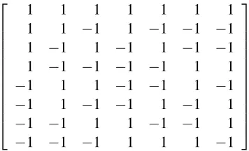
φ)|. We begin by arranging the elements ofSat(φ)as the rows of aK×nmatrix, which we will call theφ-matrix. An example of this is done for theHad3predicate in
Figure 1. The columns of this matrix are elements of {−1,1}K. Naming this setV :=
{−1,1}K, we will think ofV as the set of possible variables to be used in a gadget reduction fromφtoψ. One of the
1 1 1 1 1 1 1
1 1 −1 1 −1 −1 −1 1 −1 1 −1 1 −1 −1 1 −1 −1 −1 −1 1 1
−1 1 1 −1 −1 1 −1
−1 1 −1 −1 1 −1 1
−1 −1 1 1 −1 −1 1
−1 −1 −1 1 1 1 −1
Figure 1: TheHad3-matrix. The rows are the satisfying assignments ofHad3.
Of these variables, thenvariables found as the columns of theφ-matrix are special; they correspond
tonof the variables in the originalφinstance and are therefore calledgeneric primaryvariables. We will call themv1,v2, . . . ,vn, where they are ordered by their position in the φ-matrix. The remaining
variables are called genericauxiliaryvariables. For example, perFigure 1,(1,1,1,1,−1,−1,−1,−1)
and(1,−1,−1,1,−1,1,1,−1) are generic primary variables in any gadget reducing fromφ, but the variable(−1,−1,1,−1,1,−1,1,−1)is always a generic auxiliary variable.
On top of the variablesV there will be a distribution ofψ constraints. As a result, a gadgetGis just an
instance of the Max-ψ CSP using the variable setV. As above, we will associateGwith the distribution ofψ constraints and writeC∼Gto sample a constraint from this distribution.
Given an assignmentA:V → {0,1}, the goal is forGto be able to detect whether the valuesAassigns to the generic primary variables satisfy theφ predicate. For shorthand, we will say thatA satisfiesφwhen
φ(A(v1),A(v2), . . . ,A(vn)) =1.
On the other hand,A fails to satisfy φ when this expression evaluates to 0. Of all assignments, we
are perhaps most concerned with thedictator assignments. Thei-th dictator assignment, writtendi:
{−1,1}K → {−1,1}, is defined so thatd
i(x) =xi for allx∈ {−1,1}K. The following fact shows why the dictator assignments are so important:
Fact 2.13. Each dictator assignment disatisfiesφ.
Proof. The string((v1)i,(v2)i, . . . ,(vn)i)is thei-th row of theφ-matrix, which, by definition, satisfiesφ.
Before introducing the version we use in our reduction, we first give the standard definition of a gadget. Typically, one constructs a gadget so that the dictator assignments pass with high probability, whereas every assignment which fails to satisfyφ passes with low probability. This is formalized in the
following definition, which is essentially from [24].
Definition 2.14 (Old definition). A (c,s)-generic gadget reducing Max-φ to Max-ψ is a gadget G satisfying the following conditions.
• (Soundness) For any assignmentAwhich fails to satisfyφ,uval(A;G)≥s.
We useuvalas our focus is on the deletion version of 2-Lin(2). We include the wordgenericin this definition to distinguish it from the specific type of gadget we will use to reduceHadkto 2-Lin(2). See Section 2.3for details.
This style of gadget reduction is appropriate for the case when one is reducing from a predicate for which one knows an inapproximability result and nothing else. However, in our case we are reducing from predicates containing a balanced pairwise-independent subgroup, and Chan [7] has shownuselessness
for this class of predicates (seeTheorem 2.12). As a result, we can relax the (Soundness) condition in Definition 2.14; when reducing from this class of predicates, it is sufficient to show that this (Soundness) condition holds fordistributionsof assignments whichappear random on the generic primary variables. In the following paragraph we expand on what this means.
Denote by Aa distribution over assignmentsA. The value of A is just the average value of an assignment drawn fromA, i. e.,val(A;G):=EA∼Aval(A;G), and similarly foruval(A;G). We say thatA israndom on the generic primary variablesif the tuple
(A(v1),A(v2), . . . ,A(vn))
is, over a randomA∼A, distributed as a uniformly random element of{−1,1}n.
Definition 2.15. Denote byRgen(φ)the set of distributions which arerandom on the generic primary variables.
Our key definition is the following, which requires that our gadget only does well against distributions inRgen(φ).
Definition 2.16(New definition). A (c,s)-generic gadget reducing Max-φ to Max-ψ is a gadget G
satisfying the following properties:
• (Completeness) For every dictator assignmentdi,uval(di;G)≤c.
• (Soundness) For anyA∈Rgen(φ),uval(A;G)≥s.
The following proposition is standard, and we sketch its proof for completeness.
Proposition 2.17. Suppose there exists a(c,s)-generic gadget reducing Max-φ to Max-ψ, where Max-φ is any predicate containing a balanced pairwise-independent subgroup. Then for allε>0, given an instanceI0of Max-ψ, it isNP-hard to distinguish between the following two cases:
• (Completeness) uval(I0)≤c+ε. • (Soundness) uval(I0)≥s−ε.
Proof sketch. LetIbe an instance of the Max-φproblem produced viaTheorem 2.12. To dispense with
some annoying technicalities, we will assume that every constraintC= ((x1,b1), . . . ,(xn,bn)) in the support ofIsatisfiesbi=1 for alli=1, . . . ,n—if for somexiwe havebi=−1, then we switch the sign of its corresponding primary variable in everyψ-constraint that containsxiin the gadget forC.
Construct an instanceI0 of Max-ψ as follows: for each constraintC= ((x1,1), . . . ,(xn,1))in the
support ofI, add in a copy ofG—call itGC—whose total weight is scaled down so that it equals the weight ofC. Further, identify the primary variablesv1, . . . ,vnofGCwith the variablesx1, . . . ,xn.
Completeness. In this case, the instanceIis in the completeness case ofTheorem 2.12, so there exists an assignmentAto the variables ofIwhich violates at most anε-fraction of the constraints. We extend
this to an assignment for all the variables ofI0and show that it violates no more than a(c+ε)-fraction of
the constraints. The extension is as follows: for any constraintC= ((x1,1), . . . ,(xn,1))whichAsatisfies,
there is some dictator assignment to the variables ofGCwhich agrees withAon the primary variables
v1, . . . ,vn. SetAto also agree with this dictator assignment on the auxiliary variables inGC. Regardless
of howAis extended in the remaining gadgetsGC, it now labels a(1−ε)-fraction of theGgadgets inI0
with a dictator assignment, meaning thatuval(A;I0)≤(1−ε)·c+ε·1≤c+ε.
Soundness. LetAbe an assignment to the variables inI0. We lower-bound theuval(A;I0)by roughly
s assuming that I belongs to the soundness case of Theorem 2.12. Consider the distribution A of assignments to the gadgetG generated as follows: sample C∼I and output the restriction of Ato the variables ofGC. By the soundness case ofTheorem 2.12, the distribution(A(x1), . . . ,A(xn))isε -close to uniform in total variation distance, and thusAisε-close in total variation distance to some
distributionA0∈Rgen(φ). As a result, by the definition of a(c,s)-generic gadget, we haveuval(A;G)≥
uval(A0;G)−ε≥s−ε. But thenuval(A;G) =uval(A;I0), which is therefore bounded below bys−ε.
ByTheorem 2.12, it isNP-hard to distinguish between the two cases above for instanceI. It follows that distinguishing betweenuval(I0)≤c+εanduval(I0)≥s−ε isNP-hard.
2.2 Reducing into2-Lin(2)
In this section, we consider gadgets which reduce into the 2-Lin(2)predicate. We show several convenient simplifying assumptions that can be made in this case.
Definition 2.18. An assignmentA:{−1,1}K→ {−1,1}isfoldedifA(x) =−A(−x)for allx∈ {−1,1}K. Here−xis the bitwise negation ofx. In addition, a distributionAis folded if every assignment in its support is folded.
The following proposition shows that when designing a gadget which reduces into 2-Lin(2), it suffices to ensure that its (Soundness) condition holds for folded distributions. The proof is standard.
Proposition 2.19. For some predicateφ, supposeGis a gadget reducing Max-φ to Max-2-Lin(2) which satisfies the following two conditions:
• (Completeness) For every dictator assignment di,uval(di;G)≤c.
• (Soundness) For anyfoldedA∈Rgen(φ),uval(A;G)≥s.
Then there exists a(c,s)-generic gadget reducing Max-φto Max-2-Lin(2).
Remark 2.20. Here we are focusing onuvalinstead ofvalat the beginning ofSection 2, so thecands
here corresponds to 1−cand 1−sthere.
Proof. For each pair of antipodal pointsxand−xin{−1,1}K, pick one (say,x) arbitrarily, and set
This is the canonical variable associated toxand−x. The one constraint is that if eitherxor−xis one of the generic primary variables, then it should be chosen as the canonical variable associated toxand
−x. Defineis-canon(x)to be 1 ifcanon(x) =xand(−1)otherwise. Now, letG0 be the gadget whose constraints are sampled as follows:
1. Sample a constraintA(x1)·A(x2) =bfromG.
2. Fori∈ {1,2}, setbi=is-canon(xi).
3. Output the constraintA(canon(x1))·A(canon(x2)) =b·b1·b2.
We claim thatG0is a(c,s)-gadget reducing Max-φ to Max-2-Lin(2). Then the probability that an
assign-mentAfails onG0is the same as the probability that the assignmentA0(x):=is-canon(x)·A(canon(x))
fails onG. For any dictator functiondi,di(x) =is-canon(x)·di(canon(x))for allx. Therefore,difailsG0 with probabilityc. Next, it is easy to see that for any assignmentA,A0is folded and, due to our restriction oncanon(·),A0agrees withAon the generic primary variables. Thus, given a distributionA∈Rgen(φ),
Afails onG0with the same probability that some folded distribution inRgen(φ)fails onG, which is at
leasts.
Proposition 2.21. For fixed values of c and s, let Gbe a gadget satisfying the (Completeness) and (Soundness) conditions in the statement ofProposition 2.19. Then there exists another gadget satisfying
these conditions which only uses equality constraints.
Proof. LetG0 be the gadget which replaces each constraint inGof the formx6=ywith the constraint
x=−y. IfAis a folded assignment,
A(x)6=A(y) ⇐⇒ A(x) =A(−y).
Thus, for every folded assignmentA,val(A;G) =val(A,G0). As the (Completeness) and (Soundness) conditions inProposition 2.19only concern distributions over folded assignments, G0 satisfies these conditions.
This means that sampling fromGcan be written as(x,y)∼G, meaning that we have sampled the constraint “x=y.”
2.3 TheHadk-to-2-Lin(2)gadget
Now we focus on our main setting, which is constructing aHadk-to-2-Lin(2) gadget. ViaSection 2.2, we only need to consider how well the gadget does against folded assignments.
TheHadkpredicate has 2k−1 variables. In addition, it hasK:=2k satisfying assignments, one for each setting of the variablesx{1} throughx{k}. It will often be convenient to take an alternative (but equivalent) viewpoint of the variable setV :={−1,1}Kas the set ofk-variable Boolean functions, i. e.,
V =nf f:{−1,1}k
Remark 2.22. The variables 1K and(−1)K inV correspond to the constant functions. In what follows, when consideringgenericHadk-to-2-Lin(2)gadgets, it will be useful to view them as constants 1 and−1 in the 2-Lin(2)equations, instead of (auxiliary) variables. We argue that this is a valid simplification. Our result concerningHadk-to-2-Lin(2)gadgets consists of two parts: constructing aHadk-to-2-Lin(2) gadget in order to showNP-hardness result for Max-2-Lin(2), and prove that the gadget we constructed is optimal.
• For the first part, if we do aHadk-to-2-Lin(2)reduction using these gadgets, the 2-Lin(2)instances we get may have constraints that involve constants, such as(=)(x1,−1). A standard transformation
to turn them into ones that do not use constants is to introduce a global variablez, and replace 1 withz, −1 with−z. By changing the signs of all variables if necessary, we can always find an optimal assignment that giveszvalue 1. Thus the transformation maintains the values of the instances, and does not change the computational complexity of the problem.
• For the second part, observe that we always get gadgets at least as good by replacing the variable 1K with constant 1 and(−1)K with constant−1. The constants coincide with the dictator assignments for 1Kand(−1)K, so the completeness value does not change, and the soundness does not decrease after this simplification.
TheHadk matrix is a 2k×(2k−1)matrix whose rows are indexed by strings in{−1,1}kand whose columns are indexed by nonempty subsetsS⊆[k]. The(x,S)-entry of this matrix isχS(x). This can be verified by noting that for anyx∈ {−1,1}k,
χ{1}(x),χ{2}(x), . . . ,χ{k}(x),χ{1,2}(x), . . . ,χ{1,2,...,k}(x)
is a satisfying assignment of theHadk predicate. As a result, for eachS6=/0,χSis a column in theHadk matrix. Therefore, these functions are the generic primary variables. However, it will be convenient to consider a larger set of functions to be primary. For example, because we plan on using our gadget on folded assignments,χSand−χSwill always have opposite values, and so the−χSshould also be primary variables. In addition, it is a little unnatural to have every parity function but one as a primary variable, so we will include the constant functionχ/0and its negation−χ/0in the set of primary variables. In total, we
have the following definition. Note that in contrast to the above discussion about generic gadgets, we include the constant functions as variables in the following definition ofHadk-to-2-Lin(2)gadgets.
Definition 2.23. The variables of aHadk-to-2-Lin(2)gadget are all Boolean functions overkvariables. Theprimary variablesof aHadk-to-2-Lin(2)gadget are the functions±χS, for anyS⊆[k]. The remaining
functions are auxiliary variables.
To account for the inclusion ofχ/0as a primary variable, we will have to modify some of our definitions
fromSection 2.1. We begin by defining the following modification to theHadk predicate, and we now refer to the definition at the beginning of this subsection asHad0k.
Definition 2.24. TheHadkpredicate has 2k input variables, one for each subsetS⊆[k]. The input string
In other words, ifx/0=1, then the remaining variables should satisfy theHad0kpredicate, and ifx/0=−1,
then their negations should. We will say thatA satisfies theHadkpredicateif
Hadk A(χ/0),A χ{1}, . . . ,A χ{k},A χ{1,2}, . . . ,A χ[k]
=1.
Otherwise,A fails to satisfy theHadkpredicate. We say thatAisrandom on the primary variablesif the tuple
A(χ/0),A χ{1}
, . . . ,A χ{k}
,A χ{1,2}
, . . . ,A χ[k]
is, over a randomA∼A, distributed as a uniformly random element of{−1,1}K.
Definition 2.25. Denote byR(Hadk)the set of folded distributions which arerandom on the variables
{χS}S⊆[k].
Definition 2.26. A (c,s)-gadget reducing Max-Hadk to Max-2-Lin(2) is a gadget G satisfying the following properties:
• (Completeness) For every dictator and negated dictator assignment±di,uval(±di;G)≤c.
• (Soundness) For anyA∈R(Hadk),uval(A;G)≥s.
Proposition 2.27. The following two statements are equivalent: 1. There exists a(c,s)-gadget reducing Max-Hadk to Max-2-Lin(2).
2. There exists a(c,s)-generic gadget reducing Max-Had0k to Max-2-Lin(2).
Proof. We prove the two directions separately. Recall that the gadgets in both cases are distributions of 2-Lin(2)constraints over essentially the same set of variables, except that in (1) we have variables±χ/0,
whereas in (2), we have constants±1. To convert a gadgetGin (1) toG0in (2), we simply replace±χ/0
with±1, and vice versa.
(1)⇒(2). LetGbe a(c,s)-gadget reducing Max-Hadkto Max-2-Lin(2), andG0the corresponding(c,s) -generic gadgetG0reducing Max-Had0kto Max-2-Lin(2). We claim that for any foldedA0∈Rgen(Had0k),
uval(A0;G0)≥s. To see this, construct distribution A∈R(Hadk) as follows: sample A0 ∼A0 and
b∼ {−1,1}, output the assignmentAwhere we assignA(χ/0) =b,A(−χ/0) =−b, andA(f) =bA0(f)for
all f∈ {±/ χ/0}. By definition ofRgen(Had0k), we have thatA0is uniformly random on{χS}S6=/0, and sinceb
is uniform and independently sampled, we have thatA∈R(Hadk)and thereforeuval(A;G)≥s. We also haveA(f)A(χ/0) =A0(f)·1 andA(f)A(g) =A0(f)A0(g)for f,g∈ {±/ χ/0}, souval(A0;G0) =uval(A;G).
As a result,G0satisfies the (Completeness) and (Soundness) conditions in the statement ofProposition 2.19, meaning it is a(c,s)-generic gadget reducing Max-Had0k to Max-2-Lin(2).
(2)⇒(1). LetG0 be a(c,s)-genericgadget reducing Max-Had0k to Max-2-Lin(2), andGbe the cor-responding(c,s)-gadget reducing Max-Hadkto Max-2-Lin(2). LetA∈R(Hadk), and forb∈ {−1,1}, writeA(b)forAconditioned on the variableχ/0being assigned the valueb. Thenb·A(b)(by which we
mean the distribution where we sampleA∼A(b)and outputb·A) is inRgen(Had0k)for bothb∈ {−1,1}, and souval(b·A(b);G) =uval b·A(b);G0
≥s. Asuval(A(b);G) =uval b·A(b);G
Combining this withProposition 2.17, we have the following corollary.
Corollary 2.28. Suppose there exists a(c,s)-gadget reducing Max-Hadkto Max-2-Lin(2). Then for all
ε>0, given an instanceIof Max-2-Lin(2), it isNP-hard to distinguish between the following two cases: • (Completeness) uval(I)≤c+ε.
• (Soundness) uval(I)≥s−ε.
2.4 Reducing to the length-one case
When constructing good gadgets, we generally want dictators to pass with as high of probability as possible. ByProposition 2.21, we can assume that our gadget operates by sampling an edge(x,y)and testing equality between the two endpoints. Any such edge of Hamming distanceiwill be violated byi/K
of the dictator assignments. Intuitively, then, if we want dictators to pass with high probability, we should concentrate the probability mass of our gadgetGon edges of low Hamming distance. The following proposition shows that this is true in the extreme: so long as we are only concerned with maximizing the quantitys/c, we can always assume thatGis entirely supported on edges of Hamming distance one.
Proposition 2.29. Suppose there exists a(c,s)-gadgetGreducing Max-Hadk to Max-2-Lin(2). Then
there exists a(c0,s0)-gadget reducing Max-Hadk to Max-2-Lin(2)using only length-one edges for which
s0 c0 ≥
s c.
Proof. For eachi∈ {1, . . . ,K}, let pi be the probability that an edge sampled fromGhas lengthi, and letGidenote the distribution ofGconditioned on this event. Then sampling fromGis equivalent to first sampling a lengthiwith probabilitypi, and then sampling an edge fromGi.
LetQ=1·p1+2·p2+···+K·pK, and for eachi∈ {1, . . . ,K}defineqi=i·pi/Q. It is easy to see that theqi form a probability distribution. Now we may define the new gadgetG0as follows:
1. Sample a lengthiwith probabilityqi. 2. Sample(x,y)∼Gi.
3. Pick an arbitrary shortest pathx=x0,x1, . . . ,xi=ythrough the hypercube{−1,1}K. 4. Output a uniformly random edge(xj,xj+1)from this path.
Note thatG0 only uses length-one edges. Let G0i denote the distribution ofG0 conditioned onibeing sampled in the first step. (Note thatG0iis defined in a way that is different from the wayGiis defined.)
LetA:{−1,1}K→ {−1,1}be any assignment. Then
uval(A;G) =
K
∑
i=1
pi·uval(A;Gi), and uval(A;G0) = K
∑
i=1
qi·uval(A;G0i).
assign different values to at least one of the edges(xj,xj+1). As a result, every timeAerrs onGi, it must err at least a(1/i)-fraction of the time onG0i. This means that:
uval(A;G0i)≥uval(A;Gi)
i . (2.1)
In the case whenAis a dictator function, Equation (2.1) becomes an equality. This is becausex= x0,x1, . . . ,xi=yis a shortest path betweenx andythrough the hypercube{−1,1}K. IfAassigns the same values toxandy, then it will assign the same values to all ofx0,x1, . . . ,xi. If, on the other hand, it
assigns different values toxandy, then it will assign different values to the endpoints of exactly one edge
(xj,xj+1).
Now we can use this to relateuval(A;G0)touval(A;G):
uval(A;G0) =
K
∑
i=1
qi·uval(A;G0i)
≥
K
∑
i=1
i·pi
Q
·uval(iA;Gi)
= 1 Q
K
∑
i=1
pi·uval(A;Gi)
= 1
Quval(A;G). (2.2)
Here the inequality follows from the definition ofqiand Equation (2.1). As Equation (2.1) is an equality in the case whenAis a dictator function, we have thatuval(A;G0) = (1/Q)uval(A;G)in this case.
LetA∈R(Hadk)maximizeval(A;G0), and letdibe any dictator function. Then
s0 c0 =
uval(A;G0)
uval(di;G0) ≥ 1
Quval(A;G)
1
Quval(di;G)
=uval(A;G)
uval(di;G) ≥ s c.
Here the first inequality is by Equation (2.2) (and the fact that it is an equality for dictators), and the second inequality follows from the fact thatuval(A,G)≥sanduval(di,G) =c.
2.5 Linear programs
One of the key insights of the paper [24] is that optimal gadgets (as perDefinition 2.14) can be computed by simply solving a linear program. Fortunately, the same holds for computing optimal gadgets as per Definition 2.26. In our case, the appropriate linear program (taking into accountProposition 2.29) is:
max s
s. t. uval(A;G)≥s, ∀A∈R(Hadk),
Gis a gadget supported on edges of length one.
the linear program is simply too large to ever be feasible in practice. What is important for us is that we can take its dual; doing so yields the following linear program.
Definition 2.30. Thedual LPis defined as min s
s. t. Pr
A∼A[A(x) =A(y)]≤s, ∀edges(x,y)of length one,
A∈R(Hadk).
The dual linear program shows us that we can upper-bound the soundness of any gadget with the valuesby exhibiting a distribution on assignments inR(Hadk)which passes each length-one edge with probability at leasts. Moreover, strong LP duality tells us that the optimum values of the two LPs are the same. Hence, we can prove atightupper bound by exhibiting the right distribution. We do this in Section 4for gadgets reducing Max-Had3to Max-2-Lin(2).
2.6 TheHad3gadget
In this section, we will prove some structural results about the hypercube{−1,1}8which are relevant to
anyHad3-to-2-Lin(2)gadget. The results of this section will be useful for both Sections3and4.
Given a stringx∈ {−1,1}nand subset of stringsB
⊆ {−1,1}n, we define the distance ofxtoBas
dH(x,B):=miny∈BdH(x,y).
Let V ={−1,1}8, and let G= (V,E) be the hypercube graph, where we connect two vertices v1,v2∈ {−1,1}8with an edge if and only ifd
H(v1,v2) =1.
Definition 2.31. Given a hypercube graphG= (V,E), whereV={−1,1}8. LetV
0be the set of primary
variables of a gadget fromHad3, and for anyi>0, defineVi={x∈V |dH(x,V0) =i}. This gives a partition of vertices inV according to their distances toV0.
We can identifyV with the set of 3-variable Boolean functions. The set of primary variablesV0
corresponds to the set of affine functions, i. e., those of the form±χS, whereS⊆[3].
Proposition 2.32. For the hypercube graph G= (V,E), where V ={−1,1}8, the following holds: 1. The vertex set V can be partitioned as V =V0 ·∪V1 ·∪V2,|V0|=16,|V1|=128, and|V2|=112. 2. Each x∈V0has eight neighbors in V1.
3. Let f,g∈V0be a pair of distinct functions. Then either dH(f,g) =8, or dH(f,g) =4.
4. For any x,y∈ {−1,1}3, x6=y, bx,b
y∈ {−1,1}, the number of functions f∈V0such that f(x) =bx
is 8, and the number of functions f ∈V0such that f(x) =bxand f(y) =byis 4.
5. Each x∈V1has one neighbor in V0and seven neighbors in V2.
7. Let f ∈V2, and let g1, g2, g3, and g4be the four vertices in V0which are Hamming distance2away from f . Then for any x∈ {−1,1}3, three of the g
ifunctions have the same value and one has a
different value, and therefore f(x) =sign(g1(x) +g2(x) +g3(x) +g4(x)). We say that g1, g2, g3 and g4arethe primary variables associated with f .
Proof. In this proof, we will take the viewpoint ofV as the set of 3-variable Boolean functions.
Item (2) is straightforward—for each function f∈V0, changing any of the 8 positions would result in a function inV1by definition, and since functions inV0are at distance at least 4 from each other, their
sets of neighbors inV1do not intersect.
For item (3), suppose we have f =bfχF andg=bgχG. IfF=G, then since f6=gwe must have
f =−g, sodH(f,g) =8. Otherwise, sinceF6=G,
E
x[f(x)g(x)] =x∼{−E1,1}3[bfbgχF(x)χG(x)] =0, wherexis sampled uniformly over{−1,1}3. Thus in this cased
H(f,g) =4.
We prove item (4) by a dimension argument. A function f ∈V0can be defined as f(x1,x2,x3) = (−1)b0+b1x1+b2x2+b3x3, and we can specify f by giving the parameters b
0, b1, b2 andb3. Specifying
the value of f at a single point imposes 1 affine relation on the 4 parameters, so the number of affine functions that satisfies this constraint is 24−1=8. Specifying the values at 2 different points introduces 2
independentaffine relations and thus the resulting number of affine functions becomes 24−2=4. We now prove the remaining items. The primary variables are of the form±χS, whereS⊆[3]. There
are 16 such functions, and so|V0|=16.
Let f0 differ from one of the primary variables on a single input. It must be at least distance 3 from any of the other primary variables. This means that all its neighbors are at distance 2 or 4 from all affine functions and thus are all inV\V0\V1. There are 16·8=128 distinct ways of constructng such an f0, and so|V1|=128.
This leaves 256−16−128=112 variables inV not yet accounted for. We will now show a method for constructing exactly 112 different elements ofV2; by the pigeonhole principle, this shows thatV can be partitioned as in item (1) with the given sizes. Item (5) also follows because each function inV1has 8
neighbors, and exactly one of them is inV0. Items (6) and (7) follow naturally from the proof below.
Given three primary variablesb1χS1,b2χS2, andb3χS3, whereb1,b2,b3∈ {−1,1}, setb4:=−b1·b2·
b3andS4:=S1∆S2∆S3. Consider the function f defined as
f(x):=sign(b1χS1(x) +b2χS2(x) +b3χS3(x) +b4χS4(x)).
To see that thissign(·)is well-defined, note that by definition,∏4i=1biχSi(x) =−1 for allx∈ {−1,1}
3.
As a result, for anyx, three of thebiχSi(x)have the same value, while the other one has a different value.
This also means that for allx, we have
4
∑
i=1
biχSi(x) =2·sign
4
∑
i=1
biχSi(x)
!
.
Thus, the correlation of any of the variablesbiχSi with f is
E
x[f(x)·biχSi] = 1 2Ex
" 4
∑
i=1
biχSi(x)
! ·biχSi
# =1
In other words, Prx[f(x) =biχSi] =3/4 for eachi∈ {1, . . . ,4}. This is equivalent to saying that f is at
distance 2 from each of thebiχSi, fori=1,2,3,4.
There are 23· 83
=448 ways of selecting thebiχSi fori=1,2,3, and there are 4 different choices
ofb1χS1,b2χS2 andb3χS3 that lead to the same function. Therefore this construction gives 112 unique functions inV2. As there are only 112 functions inV which are in neitherV0norV1, all of the remaining
variables inV must be contained inV2, and they must all be generated in the manner above.
Now we consider the neighbors of f ∈V2. To get from f to each of its 4 associated functions inV0,
we need to flip 2 bits. Since we can flip them in 2 different orders, this gives all 8 neighbors of f and they are all inV1.
Proposition 2.33. Let B=sat(Had3). Then
Pr
x[dH(x,B) =0] = 1
16, Prx[dH(x,B) =1] = 1
2, and Prx[dH(x,B) =2] = 7 16,
where x is a uniformly random element of{−1,1}8.
Proof. This can be proven using a proof similar toProposition 2.32. Alternatively, we can just show a direct correspondence between the setting here and the setting inProposition 2.32, as follows.
The input to Had3 is a set of bits {xS}S⊆[k], which can also be thought of as the function f : P({1,2,3})→ {−1,1}in which f(S):=xS. The satisfying assignments are then any function of the form
S7→b·χS(x), whereb∈ {−1,1}andx∈ {−1,1}3are both fixed. For a stringx∈ {−1,1}3, letα(x)be the corresponding set, i. e.,α(S)i=−1 if and only ifi∈S. For any function f :P({1,2,3})→ {−1,1}, we can associate it with the functionα(f):{−1,1}3→ {−1,1} defined byα(f)(x):= f(α(x))for
allx. Thenα maps any satisfying assignment to Had3 into one of the primary variables inV0, and
more generally,dH(f,B) =iif and only ifα(f)∈Vi. The proposition therefore follows by applying
Proposition 2.32and by noting that 16/256=1/16, 128/256=1/2, and 112/256=7/16.
2.7 Reducing toMax-Cut
Definition 2.34. Let(6=):{−1,1}2→ {0,1}be the inequality predicate, i. e., for allx
1,x2∈ {−1,1}, (6=)(x1,x2) =1 iffx16=x2. The Max-Cut CSP is the special case of the Max-(6=)CSP in which every constraintC= ((x1,b1),(x2,b2))satisfiesb1=b2=1. In other words, every constraint is of the form
“x16=x2.”
Proposition 2.35. For some predicateφ, supposeGis(c,s)-generic gadget reducing Max-φ to Max- 2-Lin(2). Then there exists a(c0,s0)-gadget reducing Max-φ toMax-Cutsatisfying
s0 c0 =
s c.
Proof. Suppose the vertex set ofGisV={−1,1}K. LetG0be the gadget which operates as follows:
1. With probability 1−1/2K, pickx∈ {−1,1}Kand output the constraint “x6=−x.”
Any folded assignmentAfailsG0with probability at most 1/2K. Any assignmentAwhich isnotfolded failsG0with probability at least
1− 1
2K
· 2
2K > 1 2K.
As a result, we can always assume that any assignment is folded.
Now, ifAis folded, then for anyx,y∈ {−1,1}K, A(x) =A(y)if and only ifA(x)6=A(−y). As a result,uval(A;G0) =uval(A;G)/2K. Thus,c0=c/2K,s0=s/2K, and sos0/c0=s/c.
3
The factor-
11
/
8
hardness result
In this section, we prove the following theorem.
Theorem 3.1. There is a(1/8,11/64)-gadget reducingHad3to2-Lin(2).
Using Propositions2.17and2.35, we have the following two corollaries.
Corollary 3.2. There is a(c,s)-generic gadget reducingHad3toMax-Cutwith s/c=11/8.
Corollary 3.3(Theorem 1.7 restated). Fix any C<11/8. Then it isNP-hard to achieve a factor-C approximation for both the Max-2-Lin(2)and theMax-CutCSPs.
Proof ofTheorem 3.1. To construct our gadget, we will assign a nonnegative weight to each edge in the gadget. Our gadget will then sample each edge with probability equal to its weight normalized by the weight of the entire gadget. As argued inProposition 2.29, our gadget will only use length-one edges. And byProposition 2.21, our gadget will only use equality constraints. For f,g∈V withdH(f,g) =1, the weight of the edge{f,g}is 5 if and only if either f∈V0org∈V0, and otherwise the weight is 1. The
total weight of the edges inGis 5×128+896=1536.
For the completeness, the fact that the dictators pass with probability 7/8 follows immediately from the fact thatGonly uses edges of length one. For the soundness, letA∈R(Had3). We consider eachAin the support ofA, i. e., all folded assignments. We apply one of the following three lemmas lower-boundinguval(A;G)depending on the distance between the assignment to the primary variables to
Aand the satisfying assignments ofHad3.
Lemma 3.4. Let A:{−1,1}8→ {−1,1}. If the assignment of A to the primary variables satisfies the
Had3predicate, thenuval(A;G)≥1/8.
Lemma 3.5. Let A:{−1,1}8→ {−1,1}. If the assignment of A to the primary variables is distance one from satisfying theHad3predicate, thenuval(A;G)≥21/128.
Lemma 3.6. Let A:{−1,1}8→ {−1,1}. If the assignment of A to the primary variables is distance two from satisfying theHad3predicate, thenuval(A;G)≥3/16.
Proposition 2.33gives the probability that a randomA∼Awill fall into each of these three cases. In total
uval(A;G)≥ 1
16· 1 8+
1 2·
21 128+
7 16·
3 16 =
which is what the theorem guarantees.
Before proving these lemmas, we will do some preliminary work which is relevant to all three. In the remaining part of this section, letAbe some partial assignment to variables inV. We focus on partial assignments that at least assign values to all primary variables. To analyze the quality of the gadget, we analyze certain measures of the gadget and bound the best possible way to completeAto a full assignment. All definitions in the rest of this section will be with respect to the partial assignmentA.
We classify variables inV2by the assignments of their associated affine functions, where association is defined in item (7) ofProposition 2.32.
Definition 3.7. LetAbe a partial assignment, and f ∈V2be a function associated withg0,g1,g2,g3∈V0.
We say that f is a(4,0)function ifA(g0) =A(g1) =A(g2) =A(g3). We define(3,1)and(2,2)functions similarly.
We consider paths of length 2 that start at some f∈V2and end at one of the affine functionsgi∈V0. Definition 3.8. Let A be a partial assignment. A path of length 2 from f ∈V2 tog∈V0 is good if
A(f) =A(g). Otherwise it isbad.
Observe that for a function f ∈V2of type(2,2), no matter how we assign the value of f, it will
always contribute 2 good paths and 2 bad paths.
Definition 3.9. LetAbe a partial assignment that assigns value to all variables inV0and all(4,0)and
(3,1)variables inV2.
LetB0 be the number of bad paths starting from the(4,0) and(3,1)variables, and letB1 be the number of(2,2)variables. LetB:=B0+2B1. We say thatBisthe number of bad paths of assignment A. Definition 3.10. Consider a function f ∈V1 and a partial assignmentA to variables inV0∪V2. We
say that f is of type (a,b,c) if in the partial assignment, there are a good paths, b bad paths andc
undetermined-paths going through f. Note thata+b+c=7.
A function isswitchedif it has no good path through it, and isfully switchedif it is of type(0,7,0). Given a partial assignment as inDefinition 3.9, if we assign values to variables inV1 according to their closest variable inV0, then we get an assignment that violates exactly a weight ofBof edges.
Switching the assignment of f only benefits if f is of type(0,b,c), in which case switching the value of
f decreasesuvalby at most 2. Therefore, given a partial assignmentAwhose number of bad paths isB
withCswitched functions, the best way to extend it to a full assignment violates at leastB−2Cedges. The proof focuses on the partial assignment to variables inV2, since this decides both the number
of bad paths and the number of switched functions. One natural assignment is the majority assignment, where one setsA(f)for f∈V2according to the majority assignment of the four associated affine functions of f (and breaks tie arbitrarily). The overall proof idea is to show that no assignment does better than this majority assignment. In particular, we prove that no matter how we change the assignment of some of the
(4,0)and(3,1)variables to anti-majority and increase the number of bad pathsBby some numberQ, we will never be able to increase the number of functions with no good paths through them by more than
3.1 Assignments at distance 1 fromHad3
In this section, we proveLemma 3.5.
Proof ofLemma 3.5: Let Abe a partial assignment that assigns values to variables inV0, such that
there existsx0∈ {−1,1}3, andl
0∈V0, such thatA(f) = f(x0)for all f∈V0\ {l0,−l0}, andA(b·l0) = −b·l0(x0)forb∈ {−1,1}. We call±l0the corrupted affine functions.
Of the 112 functions inV2, 56 are associated with±l0, and 56 are not. The 56 functions that are not associated with±l0are all(3,1)functions by item (7) ofProposition 2.32.
Let f ∈V2be a function that is associated witha0∈ {l0,−l0}. If f is such thata0(x0)6=f(x0), then
it is a(4,0)function. There are 56/(2·2) =14 such functions. Otherwise, it is a(2,2)function. The following observation summarizes the above discussion on the types of functions inV2.
Proposition 3.11. Of the112functions in V2,56are not associated with±l0and all of these 56 have type(3,1). Of those that are associated with±l0,14have type(4,0), and the remaining42have type (2,2).
As discussed above, given a partial assignment toV0, we need to decide, for the (4,0)and(3,1)
functions inV2, whether we assign them the majority assignment. The analysis in this section proceed
in two steps. We first argue that for any assignment for the(3,1)variables, to minimize the weight of violated constraints, either all(4,0)variables are assigned according to majority of their associated functions inV0, or all of them are assigned according to anti-majority. It is then easy to argue that the
cost will be high in the case where all(4,0) variables are assigned according to anti-majority. Then, assuming that the(4,0)variables are assigned according to majority, we prove that the(3,1)variables should also be assigned according to majority. This gives us a sufficient lower-bound for the weight of violated constraints.
Let us first classify the variables inV1 with respect to the majority assignment forV2and see how
different classes of variables relate to each other. We first consider those that are neighbors of the corrupted affine functions.
Proposition 3.12. Let A be a partial assignment where variables in V2are assigned according to majority. The following properties hold:
1. Each corrupted function has1neighbor in V1of type(7,0,0)and7neighbors of type(1,0,6). This contributes a total of2functions of type(7,0,0)and14functions of type(1,0,6).
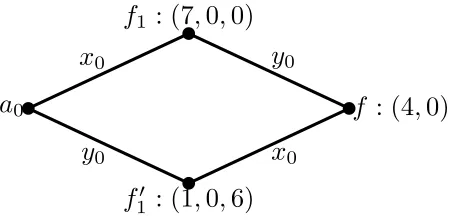
2. The(7,0,0)functions obtained by starting from±l0and flipping the value at x0. All 7 neighbors in V2of the(7,0,0)functions have type(4,0). Note that this gives a total of14functions of type (4,0), and those are exactly all the(4,0)functions.
Proof. The proof is illustrated inFigure 2.
Consider a path starting froma0∈ {±l0}. Let f1be the function obtained by flipping the value of
a0atx0. We then flip some other valuey0to get to some function f ∈V2. Since f(x0)6=a0(x0), by (7)
a
0f
1: (7
,
0
,
0)
f
1′: (1
,
0
,
6)
f
: (4
,
0)
x
0y
0y
0x
0Figure 2: The(7,0,0)and(1,0,6)neighbors of a(4,0)function.
of them end at a distinct(4,0)variable. This argument also shows that all 7V2-neighbors of f1are of (4,0)-type and hence such f1is a(7,0,0)variable.
Suppose now that we start ata0and flip the value aty0to get function f10. If we further flipx0, we
again arrive at f. On the other hand, if we flip some value other thanx0ory0, we get a function inV2of
type(2,2). This means that f10 is a(1,0,6)function.
We can now describe all neighbors of the(4,0)functions.
Proposition 3.13. Let A be a partial assignment where variables in V2are assigned according to majority. Then there are14functions in V2of type(4,0). Each of them has 1 neighbor of type(7,0,0), 1 of type (1,0,6), and 6 of type(6,0,1).
Moreover, each(6,0,1)function that is adjacent to a(4,0)function actually has 2 neighbors of type (4,0), 1 of type(2,2)and 4 of type(3,1). There are14×6/2=42such(6,0,1)functions.
Proof. FromProposition 3.12, we can obtain all(4,0)functions by starting at some corrupted affine functiona0, flipx0together with some other bity0. Let f be such a function.
We already have from the above that on the 2 paths from f toa0, we have 1 function of type(7,0,0)
and one of type(1,0,6).
To understand the other neighbors of f, consider the three affine functionsg1,g2andg3associated
with f that are nota0. We have that for anyg∈ {g1,g2,g3},g(x0)6=a0(x0)andg(y0)6=a0(y0). To each
of those affine functions there are 2 paths from f, giving a total of 6 paths. We now show that all sixV1
variables on these 6 paths have type(6,0,1).
Let f2∈V1be one of the functions on these 6 paths, and leta1be its associated affine function. We
know thata1(x0) = f2(x0)6=a0(x0),dH(f2,a0) =3. Now consider the affect of flipping different values
in f2.
• In order to get to the(7,0,0)neighbor of f from f2, we need to flip two bits. We can flip them in two different orders, so this gives us two different paths of length 2, each going through a different
(4,0)function (because(7,0,0)functions only have(4,0)neighbors).
• If we flip valuex0 of function f2and get function f0, then we have thatdH(f0,a0) =2 and thus f0is associated witha0. We also have thatdH(f0,a1) =2, so f0is also associated witha1. Note
thata1(x0)6= f0(x0) =a0(x0), which means that A(a1) =A(a0)6= f0(x0), and thus f0 is a(2,2)
• For all the otherV2-neighbors of f2, we have that they agree with f2 onx0. Also, note that the
above two cases cover all 3 paths from f2toa0. Thus for the remainingV2-neighbors of f2, we
have that they all have distance 4 froma0. This means that those functions are not associated with ±l0, and therefore are(3,1)functions contributing a good path to f2.
This concludes the analysis.
We now consider the neighbors of the uncorrupted affine functions. Note that we have already characterized some of them in the aboveProposition 3.13.
Proposition 3.14. Let A be a partial assignment where variables in V2are assigned according to majority. Then each uncorrupted affine function has4neighbors of type(3,1,3),1of type(0,4,3), and3of type (6,0,1). Functions of type(3,1,3)and(0,4,3)do not have neighbors of type(4,0).
Proof. Leta1 be an arbitrary affine function that is not corrupted, anda0now be the corrupted affine
function such thata0(x0) =a1(x0). Choose one of the four bits wherea0anda1differ, let us assume that
we have choseny0.
Starting froma1, letg1be the function where we flip the valuea1(y0). If we flip any of the three
remaining bits whereg1anda0differ, we get a function that is at distance 2 froma0, and agrees with
botha0anda1onx0. This is a(2,2)function. Otherwise, we get a(3,1)function.
There are two subcases for the latter case, in which we flip one bit thata0anda1agree on: if we flip x0and get functiong2, then taking the majority assignment forg2gives us a bad path atg1; otherwise we
get a good path.
We thus conclude that in this caseg1is a(3,1,3)function, and all good and bad paths through it are
from(3,1)functions. There are 14×4=56 such functionsg1.
Now letg0 be the function obtained by starting ata1and flipping the value atx0. If we then flip any
of the three remaining bits wherea0anda1agree, we get a function inV2 that is associated with−a0
and is of type(2,2). Otherwise, if we flip one of the 4 bits on whicha0anda1disagree, we get a(3,1)
function that contributes a bad path. This gives us 14 functions inV1of type(0,4,3).
If we start ata1and flip one of the 3 remaining bits, we get a(6,0,1)function. This completes the proof.
We have now described the types of all 128 functions inV1: 2 of type(7,0,0), 14 of type(1,0,6), 42 of type (6,0,1), 56 of type (3,1,3), and 14 of type (0,4,3). Given a partial assignment to the affine variables as well as the(4,0) and(3,1) variables inV2 (where they are assigned according to
the majority of the assignments to their associated affine functions), and a function f ∈V1, leta0 be the closest corrupted affine function, and leta1be the closest affine function. We can decide the type
of f by checking whetherdH(f,a0)is 1 or 3, whether f(x0) =a0(x0), and ifdH(f,a0) =3, whether
f(x0) =a1(x0). The details are in the above arguments and we summarize the result below.
Proposition 3.15. Fix a partial assignment as above. Let f ∈V1, a0 be its closest corrupted affine function, and a1be its closest affine function. We have the following regarding the type of f :
• If a0 =a1 and thus dH(f,a0) =1, then f has type (7,0,0) if and only if f(x0) =a0(x0), and
• If a06=a1, but a0(x0) =a1(x0) = f(x0), then f is a(3,1,3)function. • If a06=a1, f(x0)6=a1(x0), a0(x0)6=a1(x0), then f is a(0,4,3)function. • If a06=a1, f(x0) =a1(x0), a0(x0)6=a1(x0), then f is a(6,0,1)function.
Finally, we describe the neighbors of the(3,1)functions inV2.
Proposition 3.16. Let A be a partial assignment where variables in V2are assigned according to majority. Each(3,1)function contributes1good path each to3(3,1,3)functions,1good path each to3(6,0,1) functions, and1bad path to1(0,4,3)function and1bad path to1(3,1,3)function.
Proof. Let fnow be a(3,1)function. There are 6 good paths coming from it and going into 3 uncorrupted
V0variables, and 2 bad paths going to another uncorrupted variable inV0.
Consider a pair of good paths that go to the same affine functiona1. We now argue that exactly one
of the twoV1-variables is(3,1,3), and the other is(6,0,1).
Leta0be the corrupted affine function such thata1(x0) =a0(x0). Since f is a(3,1)function, it is not associated with any corrupted affine functions. Therefore, on the paths froma1to f, we flip exactly one
bitxsuch thatx6=x0anda1(x) =a0(x), and another bitysuch thata1(y)6=a0(y). ByProposition 3.15,
we have that starting froma1, if we first flipy, we get a(3,1,3)function. If we first flipx, then the closest corrupted affine function becomes−a0rather thana0, and in this case we get a(6,0,1).
Now we turn to the pair of bad paths, and leta2be the affine function at the end of the bad paths.
Note thatdH(f,a2) =2, one of the bits on which they differ isx0, and we denote the other byy. Since f is a(3,1) function, we have thatdH(f,a0) =4, therefore it must be thata0(y)6=a2(y). Therefore,
starting froma2, if we first flipx0and get function f0∈V1, then the closest corrupted affine function to f0
becomes−a0, and f0(x0) =−a2(x0) =−a0(x0), thus byProposition 3.15, the function f0is a(0,4,3)
function.
Otherwise, if we first flipy, then for the resulting function f0, the closest corrupted affine function is
a0, f0(x0) =a2(x0) =a0(x0), and therefore f0is a(3,1,3)function.
The following proposition show that in an optimal assignment, all(4,0)variables should be assigned according to majority, unless all of them are flipped.
Proposition 3.17. Let A be a partial assignment to variables in V0 as defined at the beginning of this subsection. For any partial assignment to the(3,1)and(2,2)variables, we can assume that the assignment to the(4,0)variables that minimizes the weight of violated constraints either assigns the(4,0) variables according to majority, or assigns the(4,0)variables according to the negation of majority. Proof. Fix an assignment to all variables of type(3,1)and(2,2).
We start by analyzing the majority assignment to the(4,0)variables. Under this assignment, the
(7,0,0) functions only have(4,0) neighbors and thus have 7 good paths through them. The(6,0,1)
functions have 2 neighbors of type(4,0)and thus have at least 2 good paths through each of them, and the(1,0,6)functions have at least 1 good path going through each of them.
0<k<14 of the(4,0)functions, in the best case we have madek of the(1,0,6)functions switched, and 6k/2=3kof the(6,0,1)functions switched. Note that unless we flip all(4,0)functions, we will never make the(7,0,0)functions switch. Therefore as long as 0<k<14, we will increase the number of bad paths by 8kbut will only get at most 4kmore switched functions. This means that unless we flip all assignments of(4,0)functions to anti-majority, the value of the assignment will never be better than having all(4,0)functions be assigned to majority.
Next we show that suppose the(4,0)functions are all fixed to majority, then the best assignment assigns majority to the(3,1)functions.
Proposition 3.18. Let A be a partial assignment to variables in V0 as defined at the beginning of this subsection. If all(4,0)variables in V2are assigned according to majority, then to complete this assignment and minimize the weight of violated constraints, one should set all(3,1)variables according to majority.
Proof. We start by assigning all(3,1)variables according to the majority assignments of their associated affine variables, and compare the number of bad paths introduced by each flip against the potential number of switched function we get. Note that of all the types ofV1functions we have, after setting the
(4,0)variables to majority, the only potential functions that might not have good paths through them have type(3,1,3)or(0,4,3). Note that for(0,4,3)functions, all bad paths come from(3,1)functions, thus flipping some(3,1)to non-majority only contributes good paths to some(0,4,3)functions and thus potentially decrease the number of fully switched functions. In order to upper-bound the maximum number of fully switched function, we can safely ignore the effect of those functions and only focus on the(3,1,3)functions.
Now suppose that we changekof the(3,1)functions to anti-majority assignment. Then we get 4k
extra bad paths, and the number of switched functions will increase by at most 3k/3=k<4k/2 (every flip impacts 3(3,1,3)functions, and each(3,1,3)function needs 3 flips such that the number of good paths becomes 0.) This means that in this case anything other than the majority assignment to the(3,1)
functions gives a worse assignment.
Finally, we show that flipping all(4,0)functions to anti-majority is not a good idea. In this case, the number of bad paths after assigning anti-majority to(4,0)and before assigning the(3,1)and(2,2)
functions is 14·8=112. With respect to the assignment where(4,0)functions are assigned anti-majority and(3,1)functions are assigned majority, we have 2 functions inV1of type(0,7,0), 42 functions of type (4,2,1), 14 functions of type(0,1,6), 56 of type(3,1,3)and 14 of type(0,4,3).