Impact of Distributed Generator for Loss Reduction and Improvement in Reliability of Distributed System

Impact of Distributed Generator for Loss

Reduction and Improvement in Reliability of

Distributed System

K Siva Ramudu

1

, K Mounika

2

, B Sree Ramulu

3

Assistant Professor, Department of EEE, Brindavan Institute of Technology & Science, Kurnool & JNTU – Anantapur, AP, India

UG Student, Department of EEE, Brindavan Institute of Technology & Science, Kurnool & JNTU – Anantapur, AP, India UG Student, Department of EEE, Brindavan Institute of Technology & Science, Kurnool & JNTU – Anantapur, AP, India

Abstract — Distributed Power generation has gained a lot

of attention in recent times due to constraints associated with conventional power generation and new advancements in DG technologies .The need to operate the power system economically and with optimum levels of reliability has further led to an increase in interest in Distributed Generation. By placing distributed generator on an optimal location lead to improvement in voltages. This paper investigates the impact of DG unit installation on electric losses, reliability and voltage profile of distribution networks. To find optimal distributed generator allocation for loss reduction subjected to constraint of voltage regulation in distribution network. Distributed Generator offers the additional advantage of increase in reliability levels as suggested by the improvements in various reliability indices such as SAIFI, SAIDI, CAIDI, ASAI and ASUI. Comparative studies are performed and related results are addressed. The suggested technique is programmed to IEEE-33 bus system by using MATLAB software. The results clearly indicate that DG can reduce the electrical line loss while simultaneously improving the reliability of the system. Keywords — Distributed generation, Distribution load

flows, loss Reduction, DG placement, Reliability.

I. INTRODUCTION

Distribution systems deliver power from bulk power systems to retail customers. To do this, distribution substations receive power from sub transmission lines and step down voltages with power transformers. These transformers supply primary distribution systems made up of many distribution feeders. Distribution transformers step down voltages to utilization levels and supply secondary mains or service drops [1]. Distribution planning departments at electric utilities have historically concentrated on capacity issues, focusing on designs that supply all customers at peak demand within acceptable voltage tolerances without violating equipment ratings. Capacity planning is almost always performed with rigorous analytical tools such as power flow models. Reliability, although considered important, has been a secondary concern usually addressed by adding extra capacity and feeder ties so that certain loads can be restored after a fault occurs. Although capacity planning is

important, it is only half of the story. A distribution system designed purely for capacity (and minimum safety standards) costs between 40% and 50% of a typical US overhead design [2]. This minimal system has no switching, no fuse cutouts, no tie switches, no extra capacity and no lightning protection. Poles and hardware are as inexpensive as possible, and feeders protection is limited to fuses at substations. Any money spent beyond such a "minimal capacity design" is spent to improve reliability. Viewed fr m this perspective, about 50% of the cost of a distribution system is for reliability and 50% for capacity [3]. To spend distribution reliability dollars as efficiently as capacity dollars, utilities must transition from capacity planning to integrated capacity and reliability planning4. Such a department will keep track of accurate

historical reliability data, utilize predictive reliability models, engineer systems to specific reliability targets and optimize spending based on cost per reliability benefit ratios. The impact of distribution reliability on customers is even more profound than cost. For a typical residential customer with 90 minutes of interrupted power per year, between 70 and 80 minutes will be attributable to problems occurring on the distribution systems [4]. This is largely due to the radial nature of most distribution systems, the large number of components involved, the sparsity of protection devices and sectionalizing switches and the proximity of the distribution system to end-use customers.

The main objective is to minimize the total real power loss of the system. This method is tested for IEEE 33-Bus standard test system. The tight connection between the optimal location and size is to be studied by allocating the optimal size at different buses in the network and by allocating different DG capacities at the optimal bus resulted from the proposed method [5].

1311 Reliability indices are considered to be reasonable and

logic way to judge the performance of an electrical power system [6]. Reliability indices used for the purpose of analysis in power system. The proposed methodology is tested on a standard IEEE-33 bus radial distribution system and the scenarios yields efficiency in improvement of voltage profile and reduction of power loss, it also permits an increase in reliability of the system.

II. LOADFLOWS

In this paper, a modified load-flow technique is considered for solving radial distribution networks. The proposed method involves only the evaluation of a simple algebraic expression of receiving-end voltages also node and line identification utilized [7] in load flow has been proposed. The proposed method is very efficient. It is also observed that the proposed method has good and fast convergence characteristics. The proposed method uses the simple voltage equation. The proposed method takes the zero initial loss for computation of voltage of each node and considers flat voltage start to incorporate voltage convergence.

A. Assumptions

It is assumed that three-phase radial distribution networks are balanced and represented by their single-line diagrams and charging capacitances are neglected at the distribution voltage levels.

B. Solution methodology

The load flow method of radial distribution network can be solved in three sets of equations.

1. Identification of the nodes beyond all the branches.

2. Determination of branch currents. 3. Determine the nodal voltages.

C. Procedure to determine the voltage at each bus

The distribution load flow method is used to calculate the voltage at each bus and total real and reactive power losses. Before proceeding to the fundamentals of power system control and stability limits, some factors influencing active and reactive power flows on the power system are needed to be discussed. The power transfer between two buses is related to some parameters:

• Sending and receiving bus voltages • Power angles between two buses

• Series impedances of the transmission line connecting the two buses.

Consider a single line diagram of two buses of a radial distribution system as shown in Fig.4.1, the number of branches nb and the number of buses t are related through t = nb+1. at Sth bus.

Fig 4.1: Single line diagram of two buses of a distribution system.

Where R and X are resistance and reactance of the branch. PLk and QLk are the active and reactive powers of

node k. ILi is the current flowing in the line. Subscript ‘L’

in PLS and QLS refers to the load connected

Initially, a flat voltage (1 p.u) of all the nodes is assumed and load currents and charging currents of all the loads are computed using Eqs. (3.1) and (3.2) respectively.

The load current of node k is

( )

( )

( )

* ( )

Lk L k

Lk

P

k

jQ

k

I

k

V

k

−

=

(2.1) for k = 2, 3,……. nb

Where PLk(k) and QLk(k) are active and reactive power

of load connected to node k, respectively. The charging current at node k is

I

C k

( )

k

=

y

0

( ) *

k

V k

( )

(2.2) for k = 2, 3… nb

Here shunt admittance yo is considered as small.

D. Branch current

Branch Current I(n) is equal to the sum of the load currents of all the nodes beyond that branch n plus the sum of the charging currents of all the nodes beyond that branch n i.e.,

1 1

( )

( )

( )

nb nb

Lk Ck

k n i n

I n

I

k

I

k

= + = +

=

∑

+

∑

(2.3) Where branch impedance is Z = R + j X

Therefore, if it is possible to identify the nodes beyond all the branches, it is possible to compute all the branch currents.

E. Voltage at buses

A generalized equation of receiving-end voltage, sending-end voltage, branch current and branch impedance is

V (a2) = V (a1) - I (i) * Z (i) (2.4)

Where i is the branch number and a1 and a2 are

a1 = RE (i)

a2 = SE (i)

Where RE (i) is the receiving end and SE (i) is the sending end of branch i.

F. Power losses

The real and reactive power loss of branch i are given

Lreal (i) = |I (i) |2 * R (i) (2.5)

Lreactive (i) = |I (i) |2 * X (i) (2.6)

Where Lreal (i) and Lreactive (i) are the active and reactive

power losses at branch i.

Algorithm : Identification of nodes beyond a branch Step 1. Read the system data.

Step 2. i =1

Step 3. k = i + 1, set ip = 0

Step 4. nc = 0

P

LS

+jQ

LS

P

Lk

+jQ

Lk

V

k

V

S

1311 if {RE (i) = SE(k)} and {ip = 0} go to

step 10

Otherwise go to step 12 Step 5. if {ip = 0} go to step 10

Otherwise go to step 6 Step 6. it = 1

Step 7. if {RE(i) = ie(i, ip+1)}then nc = 1

Otherwise go to step 8 Step 8. it = it +1

If {it ≤ ip} go to step 7

Otherwise go to step 9 Step 9. if {nc = 1} go to step 12 Otherwise go to step 11 Step 10. ie (i, ip + 1) = RE(i)

Step 11. ip = ip +1

IN(ip) =1

ie(i, ip + 1) = RE(i)

N(i) = ip + 1,

Step 12. s = s + 1

If {s ≤ nb} go to step 6 Otherwise go to step 13 Step 13. if {iP =0} go to step 14

Otherwise go to step 15 Step 14. ie(i, ip + 1) = RE(i)

N(i) = ip + 1, go to step 15

Step 15. i = i + 1

If {i ≤ nb-1}go to step 3 Otherwise go to step 16 Step 16. ie(nb, 1) = RE(nb) N(nb) = 1

Step 17. Stop

By using this algorithm we can find the identification of nodes beyond all branches.

III. DGPLACEMENTMETHODOLOGY

The basic idea behind the method is that when a DG is placed at a bus, the real load connected to that bus is compensated and hence the branch currents are reduced. This causes reduction in system real power loss [8]. The description of the method is given in the following sections.

A. Background

The total I2R loss (PLt) in a distribution system having n

number of branches is given by

∑

=

=

n

i

i ti

lt

I

R

P

1 2

(3.1)

Here Ii and Ri are the current magnitude of branch current

and the resistance of the ith branch. The branch current can be obtained from the load flow solution. The branch current has two components, active component (Ia) and

reactive component (Ir). The loss associated with the active

and reactive components of branch currents can be written as

PLa =

∑

=

n

i

i ai

R

I

1 2

(3.2)

PLr=

∑

=

n

i

i ri

R

I

1 2

(3.3)

Where Iai and Iri are the active and reactive components of

current of branch i.For a given configuration of a single-source radial network, the loss associated with the active component of branch currents (PL-*a) can be minimized by

placing DG units, and the loss associated with the reactive component of branch currents (PLr) can be minimized by

supplying part of the reactive power demand locally [9]. For formulating new real power and losses following formulae are derived

Pnew=Pp.u-DG Where DG is varied upto 5MW

New Spu is given by

Spu=Pnew+jQpu (3.4)

Corresponding current values is calculated as Inew=(Spu)*/(V1)*

The loss associated with the active and reactive components of branch currents can be written as

∑

=

=

n

i

i newai

a

I

R

PL

1 2

(3.5)

PLr=

∑

=

n

i

i newri

R

I

1 2

(3.6)

Where Inewai and Inewri are the active and reactive

components of current of branch i. B. Algorithm for DG Placement

Step 1: Read system data and conduct load flow analysis for the original system.

Step 2: Initialize DG=0.25 Step 3: Pnew =Ppu

Step 4: i=1

Step 5: At bus ‘i’ Pnew (i)=Ppu(i)-DG

Step 6: Conduct load flow, find the losses for new ‘P’ value.

Step 7: Check i<N if yes go to step 5 with i=i+1 else next step.

Step 8: After calculating losses for all the buses with new P values, loss with minimum

Value is assigned to ‘N’ corresponding location to ‘Y’. Step 9: Check DG=<5MW if yes go to step 3 with DG=DG+0.25 else stop.

IV.RELIABILITY

To measure system performance, the electric utility industry has developed several measures of reliability. These reliability include measures of outage duration, frequency outages, system availability, and response time performance indices, important definitions for reliability including what are momentary interruptions, momentary interruption events, and sustained interruptions [10].

• Momentary Interruption -

A single operation of an interrupting device that results in a voltage zero.

1311 An interruption of duration limited to the period required to

restore service by an interrupting device. This must be completed within five minutes.

• Sustained Interruption –

Any interruption not classified as a momentary event. The most common distribution indices include the System Average Interruption Duration Index (SAIDI), Customer Average Interruption Duration Index (CAIDI), System Average Interruption Frequency Index (SAIFI), and the Average Service Availability Index (ASAI).

A System Average Interruption Duration Index (SAIDI) The most often used performance measurement for a sustained interruption is the System Average Interruption Duration Index (SAIDI). This index measures the total duration of an interruption for the average customer during a given time period. SAIDI is normally calculated on either monthly or yearly basis; however, it can also be calculated daily, or any other time period.

To calculate SAIDI, each interruption during the time period is multiplied by the duration of the interruption to find the minutes of interruption. The customer-minutes of all interruptions are then summed to determine the total customer-minutes [11]. To find the SAIDI value, the customer-minutes are divided by the total customers. The formula is, SAIDI =Σ(ri * Ni ) / NT

Where, SAIDI = System Average Interruption Duration Index, minutes.

Σ = Summation function. ri= Restoration time, minutes.

Ni = Total number of customers interrupted. NT = Total number of customers served.

B Customer Average Interruption Duration Index (CAIDI)

Once an outage occurs the average time to restore service is found from the Customer Average Interruption Duration Index (CAIDI). CAIDI is calculated similar to SAIDI except that the denominator is the number of customers interrupted versus the total number of utility customers. CAIDI is, CAIDI =Σ(ri * Ni ) / Σ( Ni )

Where CAIDI = Customer Average Interruption Duration Index, minutes.

Σ = Summation function. ri= Restoration time, minutes.

Ni= Total number of customers interrupted.

C System Average Interruption Frequency Index (SAIFI) The System Average Interruption Frequency Index (SAIFI) is the average number of times that a system customer experiences an outage during the year (or time period under study). The SAIFI is found by divided the total number of customers interrupted by the total number of customers served. SAIFI, which is a dimensionless number, is, SAIFI =Σ(Ni) / NT

Where, SAIFI = System Average Interruption Frequency Index.

Σ = Summation function.

Ni= Total number of customers

interrupted.

NT = Total number of customers served.

D Average Service Availability Index (ASAI)

The Average Service Availability Index (ASAI) is the ratio of the total number of customer hours that service was available during a given time period to the total customer hours demanded [12]. This is sometimes called the service reliability index. The ASAI is usually calculated on either a monthly basis (730 hours) or a yearly basis (8,760 hours), but can be calculated for any time period. The ASAI is found as, ASAI = [1 – (Σ (ri * Ni) / (NT* T))] * 100

Where, ASAI = Average System Availability Index, percent.

Σ = Summation function.

T = Time period under study, hours. ri= Restoration time, hours.

Ni = Total number of customers interrupted. NT = Total number of customers served.

V. RESULTANALYSIS

The proposed model is tested on IEEE-33 bus system. For this we require system data. Data for 33-bus system. Figure 1 shows the IEEE standard 33 bus system.

Number of busses=33; Number of branches=32; Base voltage=12.66 kV; Base MVA=5.246 MVA;

Fig.1: Single Line Diagram of the Test Network

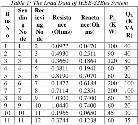
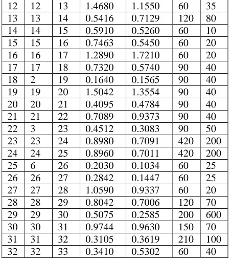
Table 1: The Load Data of IEEE-33Bus System

B us N

o Sen din g No de

Rec ievi ng No

de

Resista nce (Ohms)

Reacta nce(Oh ms)

PL

(K W)

QL

(K VA

R)

1 1 2 0.0922 0.0470 100 60

2 2 3 0.4930 0.2511 90 40

3 3 4 0.3660 0.1864 120 80

4 4 5 0.3811 0.1941 60 30

5 5 6 0.8190 0.7070 60 20

6 6 7 0.1872 0.6188 200 100

7 7 8 0.7114 0.2351 200 100

8 8 9 1.0300 0.7400 60 20

9 9 10 1.0440 0.7400 60 20

10 10 11 0.1966 0.0650 45 30

1311

12 12 13 1.4680 1.1550 60 35

13 13 14 0.5416 0.7129 120 80

14 14 15 0.5910 0.5260 60 10

15 15 16 0.7463 0.5450 60 20

16 16 17 1.2890 1.7210 60 20

17 17 18 0.7320 0.5740 90 40

18 2 19 0.1640 0.1565 90 40

19 19 20 1.5042 1.3554 90 40

20 20 21 0.4095 0.4784 90 40

21 21 22 0.7089 0.9373 90 40

22 3 23 0.4512 0.3083 90 50

23 23 24 0.8980 0.7091 420 200 24 24 25 0.8960 0.7011 420 200

25 6 26 0.2030 0.1034 60 25

26 26 27 0.2842 0.1447 60 25

27 27 28 1.0590 0.9337 60 20

28 28 29 0.8042 0.7006 120 70 29 29 30 0.5075 0.2585 200 600 30 30 31 0.9744 0.9630 150 70 31 31 32 0.3105 0.3619 210 100

32 32 33 0.3410 0.5302 60 40

First load flow is conducted for IEEE-33 bus test system. The power loss due to active component of current is 136.9836 kW and power loss due to reactive component of the current is 66.9252 kW. A programme is written in MATLAB by using load flow algorithm which is discussed above. By executing that programme total loss in the power system and p.u nodal voltages are obtained and listed in Table 2.

Table 2: Total losses of 33-Bus system from load flows

Loss due to real part of I in kW

Loss due to reactive part of I in kVAR

Total loss in kW

136.9836 66.9252 203.9088

Fig 2: p.u Nodal Voltages

A program is written in “MATLAB” to implement single DG placement algorithm [13]. For the first iteration the maximum saving is occurring at bus 6. The candidate location for DG is bus 6 with a loss saving of 93.8323 kW.

Table 3: Optimal Locations and Losses for Corresponding Dg Size

DG

size 0.25 0.50 0.75 1.00 1.25 1.50 1.75 Opt.

Loca tion

17 15 14 30 30 29 8

Loss with DG

107. 2

86.89 1

73.49 1

64.66 4

57.8 21

54.08 9

50.32 9

DG size 2.00 2.25 2.50 2.75 3.00 3.25 3.5

Opt. Locatio n

7 6 6 6 6 6 6

Loss with DG

46.7 88

44.3 78

43.1 86

43.6 74

45.8 07

49.5 53

54.8 79

DG size 3.75 4.00 4.25 4.50 4.75 5.00

Opt.

Location 6 6 6 5 4 3 Loss with

DG

61.7 54

70.1 48

80.0 32

88.6 85

93.7 88

97.2 74

The results of the DG placement method by proposed method are shown below table.

Table 4: DG Placement Method Results of 33 bus system

DG Location 6

DG Size(MW) 2.5601

PLt PLa PLr

Loss Before DG Placement(kW)

203.9088 136.9836 66.9252

Loss After DG

Placement(kW) 105.0924 43.1513 61.8781 % Reduction

in Loss 48.46 68.498 7.5336

By placing 2.5601 MW DG unit at Bus 6 the total real power loss is reduced to 105.0924 kW from 203.9088 kW and the loss associated with active component of the branch current (PLa) is reduced to 43.1513 kW from

136.9836 kW. The reduction in total power loss is 48.46% and 68.498% reduction is achieved in the loss associated with active component of the branch current (PLa) [14, 15].

The reduction in the loss associated with reactive component of the branch current (PLr) is very small as it is

1311

Fig.2: Voltage Profile with and without DG unit

The results of proposed method are shown in the Table 5 and can be compared with the results associated without DG. It can be seen from the results that the reliability indices will experience considerable changes when DG modelling is changed. Comparing the failure rates and unavailability associated with two cases of with and without DG installation, it can be seen that DG installation can improve reliability indices considerably especially SAIFI, SAIDI & ASUI and the effects are more obvious for ending sections of the feeder [16].

VI.CONCLUSION

Use of distributed generation is one of the many strategies electric utilities are considering to operate their systems in the deregulated environment. Inclusion of DG at the distribution level results in several benefits, among which are congestion relief, loss reduction; voltages profile improvement and improvement in reliability. This project has considered the benefit of DG on loss reduction, voltage improvement and Reliability for a simple case of a radial distribution line. The results clearly indicate that DG can reduce the electrical line loss while simultaneously improving the reliability of the system. However, the inclusion of DG does not always guarantee the reduced line loss. The DG rating and location are important factors for line loss reduction. Therefore, these factors have to be considered very carefully in order to determine the best location of DG. The improvement in reliability indices is maximum with DG at feeder end. Power losses decrease as location of DG from feeder end increases. We arrived at an optimal location by keeping into account these two mutually opposing factors.

REFERENCES

[1] CIGRE WG 37–23, “Impact of increasing contribution of is persed generation on power system”, final report’, September 1998.

[2] Dugan R.C., Price S.K.: ‘Issues for distributed generations in the US’. Proc. IEEE PES, Winter Meeting, January 2002, vol. 1, pp. 121–126.

[3] M. Fotuhi-Firuzabad, A. Rajabi-Ghahnavie, “An Analytical Method to Consider DG Impacts on

Distribution System Reliability” IEEE/PES Displacement and Distribution Conference & Exhibition, Asia and Pacefic, vol. 9, 2005, pp.1-6. [4] E. Diaz-Dorado, J. Cidras, E. Miguez, “Application

of evolutionary algorithms for the planning of urban distribution networks of medium voltage”, IEEE Trans. Power Systems , vol.17,no.3, pp.879-884,Aug 2002.

[5] M. Mardaneh, G. B. Gharehpetian, “Siting and sizing of DG units using GA and OPF based technique,” TENCON. IEEE Region 10 Conference,vol.3,pp.331-334,21- 24,Nov.2004.

[6] Silvestri A.Berizzi, S.Buonanno, “Distributed generation planning using genetic algorithms” Electric PowerEngineering, Power Tech Budapest 99, Inter. Conference, pp.257,1999.

[7] Das D., Kothari D.P. and Kalam A., “Simple and efficient method for load flow solution of radial distribution networks”, Electrical Power & Energy Systems, vol. 17, no. 5, pp. 335-346,1995.

[8] K. Siva Ramudu1, M. Padma Lalitha2, P. Suresh Babu “Siting and Sizing of DG for Loss Reduction and Voltage Sag Mitigation in RDS Using ABC Algorithm” International Journal of Electrical and Computer Engineering (IJECE) Vol. 3, No. 6, December 2013, pp. 814~822.

[9] K. Siva Ramudu1, M. Padma Lalitha2, P. Suresh Babu “Optimal Placement of DG for Loss Reduction and Voltage Sag Mitigation in Radial Distribution Systems using ABC Algorithm” ACEEE Int. J. on Electrical and Power Engineering , Vol. 5, No. 1, February 2014.

[10] K. Siva Ramudu1, M. Padma Lalitha2, P. Suresh Babu “Siting and Sizing of DG for Loss Reduction and Voltage Sag Mitigation in RDS Using ABC Algorithm” Proceedings of 10th IRAJ International Conference, 27th October 2013, Tirupati, India. ISBN: 978-93-82702-36-8.

[11] M.Padma Lalitha,V.C.Veera Reddy, N.Usha“Optimal DG placement for maximum lossreduction in radial distribution system”International journal of emerging technologies& applications in engineering, technology & sciences, Vol 2,Issue 2, Jul 2009, pp:719-723.

[12] Dervis Karaboga and Bahriye Basturk, “Artificial Bee Colony (ABC)Optimization Algorithm for Solving Constrained Optimization Problems,”Springer-Verlag, IFSA 2007, LNAI 4529, pp. 789–798, 2007.

[13] Karaboga, D. and Basturk, B., “On the performance of artificial bee colony(ABC) algorithm,” Elsevier Applied Soft Computing, Vol. 8, pp.687–697,2007. [14] Hemamalini S and Sishaj P Simon., “Economic load

dispatch with valve-pointeffect using artificial bee colony algorithm,” xxxii national systems conference,NSC 2008, pp.17-19, 2008.

[15] Fahad S. Abu-Mouti and M. E. El-Hawary “Optimal Distributed GenerationAllocation and Sizing in Distribution Systems via artificial bee 0 5 10 15 20 25 30 35

0.91 0.92 0.93 0.94 0.95 0.96 0.97 0.98 0.99 1

Bus Number

V

o

lt

a

g

e

M

a

g

n

it

u

d

e

i

n

p

.u

Voltage Profile With & Without DG Unit

1311 Colonyalgorithm,” IEEE transactions on power

delivery, Vol. 26, No. 4, 2011.