Development of Computational Model to Predict Rut Formation using GIS for Planning of Wood Harvesting on Drained Peat lands

(1)

Infogain Publication (Infogainpublication.com) ISSN : 2454-1311

Development of Computational Model to Predict

Rut Formation using GIS for Planning of Wood

Harvesting on Drained Peat lands

Teijo Palander

1

, Kalle Kärhä

2

Professor in forest Technology, University of Eastern Finland, Faculty of Science and Forestry, P.O. Box 111, FI-80101 Joensuu, Finland.

Development manager, Stora Enso Wood Supply Finland, P.O. Box 309, FI-00101 Helsinki, Finland.

Abstract— Modern computerized planning systems are

necessary for wood procurement of forest industry in the near future. The purpose of this study was to examine if planning of wood harvesting from peat land thinning could be digitized by GIS, when the success criterion is a rut formation in stands caused by harvesting machinery: 1) a maximum rut depth and/or 2) the percentage of formatted rut of total strip road length. The aim was to develop the computational model of rut formation for stand selection in summertime harvesting. The variables of the model described harvesting conditions, which are usually measured using field measurements. It was also aimed that this manual work could be replaced by utilizing digitized geographical information. To perform the study, harvesting conditions, as well as harvesting results including the rut formation were collected in each stand. The forwarding distance, thickness of peat layer and a depth to the groundwater table had a significant effect on the rut formation. Furthermore, the carrying capacity class of harvesting machinery, the quality of brush mat, trees’ stumps, and bends on strip road network contributed to the depth of ruts. The rut formation was correlated witha laser pulse density returning from the vegetation (2×2 m raster)and the ground height model (2×2 m) produced by an airborne laser scanning. The height information and the groundwater data were combined as a new independent variable, because the model of maximum rut depth was statistically more significant and, consequently, the stand selection was more reliable. However, on the basis of the study results, the use of airborne laser scanning for digitization of enterprise resource planning systems requires manual support of the field measurements for reliable wood harvesting operations of peat land thinnings. Even with decision support of manual field measurements 14% of stand selections would have been wrong. Besides, harvesting machinery with a low nominal ground pressure (<30 kPa) is necessary for successful harvesting operations.

Keywords— ALS, GIS, GRL, digitalization, forest operations, modelling, planning system.

I. INTRODUCTION

Operational environment

The national forest programme in Finland has set a goal to increase the amounts of industrialwood harvesting from the current level(around 60 million m3solid over bark (sob)) to 65–70 million m3sobby 2020 (Finland’sNational Forest Programme 2011). Achieving the challenging target requires increasing the wood harvesting volumes from peatland forests. From the total area in Finland34% is classified as peatlands(24% from total growing stock volume). Moreover, currently there are approximately 200,000 hectares of first-thinning stands on drained peatlands waiting for wood harvesting operation (Heikkilä 2007;Kaila &Ihalainen 2014). It can be calculated that during the 21st century the annual wood harvesting volume from peat land forests has been around 5–7 million m3 sob. According to the latestestimations (Heikkilä 2007), the annual wood harvesting volume on peatlands could be doubled (i.e. 12–14 million m3sob) in Finland.

Typically, wood harvesting operations from peat land forests have been carried out in wintertime during the coldest period in Finland. Therefore, wood harvesting operations lead to a strong seasonal variation, which has decreased cost-efficiency of Finnish wood procurement (Palander et al. 2012b). What is more, harvesting conditions are changing, because summers are lasting longer and frost is reducing during winter when climate is warming(Gregow et al. 2013). Hence, the appropriate period for winter time wood harvesting will shorten. In order to resolve these challenges, it has been suggested that the summertime wood harvesting should be increasedby developing better classification systems of peat land thinnings, which could be used indecision support systems (Heikkilä 2007).

(2)

International Journal of Advanced Engineering, Management and Science (IJAEMS) [Vol-2, Issue-12, Dec- 2016] Infogain Publication (Infogainpublication.com) ISSN : 2454-1311

www.ijaems.com Page | 2041 guidelines of successful harvesting results for thinning

stands, the acceptable rut formation will be interpreted as lower than 10 cm deep and shorter than 50 cm long ruts (Korjuujälkiharvennushakkuussa… 2003). On the other hand,the share of formatted ruts in the stand is not allowed to exceed 4% of the total length of strip roads in the stand(PEFC FI… 2014).Furthermore, according to the new criteria forwood harvesting from Scots

pine-dominated (PinussilvestrisL.) peatlands damagesare allowed to the percentage of formatted ruts contribution by 10%. In this study, we measured and calculated both 1) the maximum rut depth (cm) and 2) the percentage of formatted rut of total strip road length, i.e. the rut formation percentage (%), and which together are referred to as the rut formation.

Fig.1: Rut formation of thinning stand during summertime wood harvesting on drained peat land.

The rut formation can occur as a strengthening of the soil, but according toSaarilahti (1991) the rut formation refers to the transition of tyres onto the soil. If the shear modulus of surface layer is exceeded, a wheel sink deeper, until the settlement into an oppositional force or load-bearing capacity is the amount of load on the response. The shear modulus means the property of ground that opposesinternal deformation. According to Saarilahti (1991), the shear modulus of peat soil is high, but the load-carrying capacity is low. In terms of wood harvesting, it is crucial to ensure that the top layer of peat remains intact, because driving of the machine against the surface layer requires more power and fuel consumption (Yong 1984; Saarilahti 1991). Therefore, if the harvesting machine sinks, this reduces the productivity and cost-efficiencyof wood harvesting. Harvesting operations can also be delayed in which case timber left on harvesting site will cause a reduction in a quality of timber, too. Sometimes, wood procurement organisations must pay compensations to forest ownerswhen the promised wood harvesting date is not realized.

The rut formation has been found to increase when the thickness of the peat layer increases (Lindeman 2010; Sirén et al. 2013). Wetness of peat layer deduces the shear modulus of peat. Hence,lowering of a depth to the groundwater table reduces rut formation (Saarilahti 1991; Lindeman 2010). From the point of view of the load-bearing capacity, the structure of the surface layer of peat is crucial, because the shear modulus of peat is not just adequate for wood harvesting (Yong et al. 1984). The

properties of soil on peatlands, such as ground vegetation and the root systems of trees,will affect the soil bearing capacity of top layer. That is why in the investigation by Lamminen (2008) the thickness of peat layer did not have any significant impact on rut formation. Tree volume in stand per hectare and the amount of logging residues processed or transferred to the strip road have been found to have the impact on the reduction of rut formation (Airavaara et al. 2008; Lamminen 2008; Kärhä &Poikela 2010; Kärhä et al. 2010; Lindeman 2010; Ala-Ilomäki et al. 2011; Sirén et al. 2013;Uusitalo& Ala-Ilomäki 2013). On the other hand, an increasingwood removal per hectare can add rut formation, because anumber of passes with forwarder increases. For this reason, the removal in the stand is unclearly interpreted as a factor for the reduction of rut formation. According to the study by Sirén et al. (1987), there is a significant dependence between the number of forwarding passes and the rut formation caused by harvesting machinery.

Harvesting machinery for peat lands

(3)

Infogain Publication (Infogainpublication.com) ISSN : 2454-1311 harvesting machines for summertime harvesting on peat

lands have already been developed. According to him, tracked machines seem to be better than wheeled machines for peat lands’ thinnings, because ground pressure in these machines is divided more evenly into ground than with the wheeled machine units.

On the basis of the investigation of the available literature for harvesting machine types and models, there are significant differences between nominal ground pressures of machinery and rut formation caused by machinery (Sirén et al. 1987; Airavaara et al. 2008; Lamminen 2008; Lindeman 2010; Ala-Ilomäki et al. 2011; Palander et al.2012b). Generally speaking, thinning harvesters and harvesters based on tracked excavators are considered as suitable machines for summertime cuttings on peatlands (Bergroth et al. 2007;Ojasalo 2007; Palander et al. 2012a; Uusitalo et al. 2015). In the same studies, it was recommended light forwarders equipped with at least eight wheels and as wide tracks as possiblefor wood haulage from piles of peatlands to roadside storages.Bergroth et al. (2007) have found that the harvesters based on tracked excavator fit well summertime operations due to the good carrying capacity of their track systems. Airava ara et al. (2008) have emphasized that the good shaped tracks improve significantly the carrying capacity of forwarder. In the study by Sirén et al. (1987) 8-wheeled forwarders equipped with tracks came off mainly better than 6-wheeled ones. In Lindeman’s study (2010) 6-6-wheeled forwarders caused about 30% of the deeper ruts than 8- and 10-wheeled ones(Palander et al. 2012b).

Planning of peatland harvesting operations

The digitization of enterprise resource planning informationincluding Internet of Thingshas made it possible to utilize new information sources like GIS-datain planning of wood procurement. However, currently there are no comprehensive studies about these tools and their usefulness in summertime harvesting operations on peat lands. For example, could GIS-data be used to develop the current classification of nominal ground pressures of harvesting machinery? For this purpose it would be useful to model rut formation caused by machinery for more advanced planning system sat the

stand level. By means of airborne laser scanning (ALS) it has been suggested that the amount of the internal variation of height in the stand, as well as the spatial variation of tree volume and basal area in the stand have an effect on rut formation (Haavistoet al. 2011; Uusitalo et al. 2012). However, Salmi (2011) has underlined that it is hard to find exposed spots for rut formation on harvesting site by means of harvesting circumstance factors produced by the actual height model (25×25 m).On the other hand, gamma ray logging (GRL) has provided interesting digital information for computerized modelling (Virtanen 1990; Hyvönen et al. 2005).In this respect, Ala-Ilomäki (2005) has emphasized that the current gamma radiation maps are too broad-mindedfor an evaluation of rut formation. Kokkila (2011) has, nonetheless, proposed that it would be worthwhile to test gamma radiation data and the basic soil maps for illustration of spatial variability on harvesting site. Besides she has suggested in the same studythat more accurate height model (2×2 m)should be considered as an experiment of wood harvesting planning.

In practice, managers of wood procurement organisations execute harvesting planning of stands using field measurements. They also utilize the current classification for forwarders with different level of nominal ground pressures presented in Table 1.Airavaara et al. (2008) have even pointed out that forwarder’s load size should be determined by the impact of load to the axis masses and the nominal ground pressures. During actual planning process of stand the carrying capacity classification for harvesting sites and wood harvesting machinery is determined applying Table 2 (Högnäs et al. 2009). From the same study material (Högnäs et al. 2009), the basic models for estimation of rut formation has been drawn up by Lindeman (2010). Using Table 2a suitable forwarder can be selected specifically for thinning of a stand in summertime wood harvesting operations on drained peat lands. During the classification process managers need to pay attention on tree volume per hectare in prior harvesting operation, harvesting machinery, depth to the groundwater table, four weeks of rainfall, peat layer depth, and strip road network on harvesting site.

Table.1: The carrying capacity rates for forwarders (eight wheels) with 8-tonne load, when own mass of a forwarder is 12 and 17 tonnes (Airavaara et al. 2008). Maximum nominal ground pressure: Class 1 ≤ 50 kPa, Class 2 ≤ 40 kPa,Class 3 ≤ 30

kPa.

Class 1 Class 2 Class 3

• 12 t: in front the chains and in rear ≥700 mm wide tracks.

• 17 t: in front and in rear ≥700 mm wide tracks.

• 12 t: in front the chains and in rear ≥750 mm wide tracks.

• 17 t: in front and in rear ≥870 mm wide tracks.

• 12 t: in front ≥700 mm wide tracks and in rear ≥700 mm wide tracks with extra axle.

(4)

www.ijaems.com Page | 2043 Table.2: The carrying capacity classification for harvesting sites and wood harvesting machinery on peatland thinnings (Högnäs et al. 2009). Classes from 1 to 3 represent the required carrying capacity of harvesting machine in specific stand

harvesting conditions.

Initial tree volume, m3ha-1

Estimated load on strip road network based on the storage, shape and size of harvesting site *), **)

Low Moderate High

Carrying capacity class of forwarder

>170 1 2 3

170–120 2 3 WINTER

<120 3 WINTER WINTER

Patches for theclasses:

- Depth to the groundwater table:

• If the groundwater table is less than 25 cm depth in the swamp's surface, the carrying capacity willdecrease by one grade.

• If the harvesting operation has been preceded by a dry season which has lasted for more than 4 weeks, the carrying capacity will increase by one grade.

- If the thickness of peat layer is less than 75 cm, the carrying capacity will increase by one grade. - Timber haulage in forest

*) Average forest haulage distance on peatland: low <100 m, moderate 100 – 200 m, and high > 200 m.

* *) It is assumed that logging residues are cut to strip roads and small-sized and critical points on strip road network shall be reinforced by logging residues or in any other way.

Aims of study

A general soil map in Finland (1:20,000) consists of a lot useful information for conventional planning of wood harvesting operations on drained peatlands (Saarelainen 1998). Correspondingly, more accurate basic soil map (1:10,000) is better for planning small stands. The purpose of this study was to examine if harvesting planningsystems could be developed by digital information of modern GIS, e.g. ALS and GRL data. When planning of wood harvesting operations is done for thinnings on peatlandsto avoid rut formation, it is crucial to know, is astand suited either for summertime or wintertime harvesting, because rut formation usually occurs during summer. Therefore, the study examined what factors causedthe rut formation and could factors’ relationships be modelled using digital data forsummertime harvesting of stands on drained peatlands. For this purpose, in addition to GIS data, the data of harvesting conditions and cutting results were collected from harvested stands. By applying these factors several computational models of rut formation was evaluated and tested by selecting stands for summertime harvesting.

II. MATERIAL AND METHODS

Digital data of geographical information

Finland is covered by soil maps in scales from 1:10,000 to1:200,000. In this map, the numerical soil type patterns (≥6.25 ha) have been produced for the maps, and related property and the quality information of the available data largely by interpreting, editing and making use of existing geophysical data sets of GIS and image processing

techniques. Amendments (corrections and additions) have also been made by a geographic position system (GPS) and by mapping in the field. From point of view for wood harvesting planning, it is displayed both surface soils and ground layerson the maps. Furthermore, topographic database has been used for description of peatlands and paludificatedareas, as well as geophysical data for determination of thickness of peat layer.

In the whole country ofFinland, magnetic, electronic and radio-metric measurements havebeen produced by airborne geophysical mapping. These soil mapping flights was systematically carried out since 1972 in which flights’ height havebeen between 30–50 m and the distance of flight lines 200 m. All mineral soils are, to varying degrees, radioactive. That is why the radioactive elements and the isotopes of mineral soil emit short-wave electromagnetic radiance. This gamma radiation data are interpolated on the size of the 50×50 m raster for different maps (Hyvönen et al. 2005). In this study, the radiation of potassium and other components of the material were used to take advantage of the thickness of peat layer and identification of wetland areas. The water content of peat is, on average, 90%. That is why from the peat bogs of the natural humidity the gamma rays are impossible to detect by GRL, if the peat layer thickness is more than 0.6 m (Virtanen 1990; Virtanen &Vanne 2008).

(5)

Infogain Publication (Infogainpublication.com) ISSN : 2454-1311 back to the laser scanner, which can be used to specify a

location for the item receiving the pulse hits and the height of the scanner based on the location information and the laser pulse time travelled. Scanner measures also the strength of the return pulse. In this case, the set of all the items in the specified items in the box, which represents the laser pulse is a hit and did not reflect the return of pulses. The coordinate of individual laser pulses can be converted to terrestrial coordinate systems for the height findings. Such as a point cloud obtained from processing reflections and/or from echoes, it is possible to form the continuous surface models, such as the ground height model and the stand height model (Hyyppä&Inkinen 1999). The values of the height models are usually underestimates, because the laser pulse may not always hit the top of the tree (Hyyppä et al. 2001). The following height models were used in this study: the model of ground surface (2×2 m), the height model of trees (2×2 m), as well as a descriptive model produced by laser pulse (6×6 m). The models were produced using ALS infra-red pulse, while the laser scanning density had a minimum of 0.5 m-2. The tree models reflected from the

vegetation, which were more than two metres height.The accuracy of the height information was approximately ±30 cm. The laser grid of the stand was in use from limited study area,especially, when the laser grid micro patterns (2×2 m)were produced on map level. This data included among others the number of trees, the density of trees in the stand, the basal area of whole stand and the basal area of tree species.

For the determination of the location of the plots of stands a systematic point network (50×50 m)was created bya "Create a fishnet" tool of the ArcGis program (Table 3). More than a dozen acres of harvesting sitethe network density was reduced to 100 m. Points were established on the plots so that the plot was to be measured to the nearest strip road. Plots were established on the 240 ones (total 3.5 ha). General soil map (1:200,000) was available in all study plots. Also the height model (25×25 m) was available in all study plots, but it was only used in the calculation of the depth of the groundwater table and in the calculation of the variation of the internal topographic height of the harvesting site just there, where more accurate height material (2×2 m) was not available. Table.3: The number of the study plots (N)for digital geographical information of stands.

Data source Plot, N

Raster of the length of the stand 96

Densityraster 85

Potassiumraster 179

General soilmap(1:200,000) 240

Heightraster (2×2m) 96

Heightraster(25×25m) 144

Harvesting conditions in the study stands

The stands of the study located in the provinces of South Karelia, North Karelia, South Karelia, North Karelia and North Ostrobothni a in Finland. The tree volume per hectare, harvesting method and removal per hectare were collected from the harvesting sites of the stands. Tree volume of stand in prior harvesting operation was an average of 150 m3 ha-1 (variation range: 19–265 m3ha-1) (Figure 2). The average forest haulage distances and the distances between ditches was established on the map.

Fig.2: Tree volume per hectare in prior harvesting operation by study stand.

The depth to the groundwater table was measured by digging a pit close to the plot in each study stand. The digging place was chosen ocularly from deepest place of the stand. The thickness of peat layer was measured by peat sampler in the middle of each plot. A class of 100 cm were the largest part of the findings, with the thickness of the peat layer also surpassing 100 cm (Figure 3). Otherwise, the thickness of the peat frequency distribution was almost statistically normally distributed.

Fig.3: The frequency of measured thickness of peat layers in the study stand. When the depth of peat layer more than 100 cm in the stand, it observation has been combined to

(6)

International Journal of Advanced Engineering, Management and Science (IJAEMS) [Vol Infogain Publication (Infogainpublication.com

www.ijaems.com The model of a machine, the number of wheels and tracks

used in harvesting machinery (i.e. harvesters,

and harwarder of study) were examined. Three different

Table.4: The model and the number of wheels used in harvesting machinery of the study, as wells as the number of plots in the study. Typ

Machineunit John Deere 1070D PonsseBeaver Ponsse HS10Cobra John Deere 1010D John Deere 810D PonsseElk

Ponsse S10Caribou PonsseWisent PonsseGazelle

Valmet 840 + pullingtrailer

Fig.4: Typical 8

Harvesting results from the study stands

The harvesting result data were collected from the stands where wood harvesting operations had carried out during the summers of 2011 and 2012. From the middle of the plot six meters of strip road in both directions measured. The length of rut formation was determined from this trip (i.e. 12 m). The percentage of rut formation of stand was calculated by means of the length of rut formation according to the guidelines of harvesting result in thinnings drawn up by Metsäteho (Korjuujälkiharvennushakkuussa…2003). The rut formation was measured from longer than 50 cm long ruts if it could be found on one of tracks. Besides, the deepest rut point (i.e. maximum rut depth) on the tracks was measured, as well as the average rut depth was estimated The average percentage of formatted rut of

length was 12% in the study stands. Respectively, the maximum rut depth, on the average, was11

deviation was 11 cm)(Figure 5), while depth of plots was 4 cm (standard deviation The highest percentage of formatted rut of stand

of Advanced Engineering, Management and Science (IJAEMS) [Vol Infogainpublication.com)

, the number of wheels and tracks

machinery (i.e. harvesters, forwarders . Three different

harvester models and six different used in the study stands (T forwarders were 8-wheeled ones

The model and the number of wheels used in harvesting machinery of the study, as wells as the number of plots in the study. Type: H = Harvester; F = Forwarder;HF = Harwarder.

Type Wheel, N

H 6

H 8

F 8

HF 8

F 12

Typical 8-wheeledforwarder on Finnish peatlands.

from the study stands

ing result data were collected from the stands erations had carried out during . From the middle of the six meters of strip road in both directions was The length of rut formation was determined from this trip (i.e. 12 m). The percentage of rut formation was calculated by means of the length of rut uidelines of harvesting results Metsäteho Ltd. . The rut than 50 cm long ruts Besides, the deepest rut point (i.e. maximum rut depth) on the tracks was as well as the average rut depth was estimated.

percentage of formatted rut of total strip road . Respectively, the 11 cm (standard the average rut standard deviation was 5 cm). of stand was 56%

(standard deviation was 23 largest maximum rut depth was

Fig.5: The frequency of measured maximum rut depth in the plots of study stand

The width of strip road was

Observations of the width of strip road

determining the distance to the nearest tree of strip road on both sides of the central line, and by

of Advanced Engineering, Management and Science (IJAEMS) [Vol-2, Issue-12, Dec- 2016] ISSN : 2454-1311

Page | 2045 different forwarder modelswere used in the study stands (Table 4). In this study, all

ones (Figure 4).

The model and the number of wheels used in harvesting machinery of the study, as wells as the number of plots in .

Plot, N 77 14 124 14 57 6 100 14 62 24

23%). Correspondingly, the was 75 cm.

The frequency of measured maximum rut depth in study stands.

(7)

Infogain Publication (Infogainpublication.com) ISSN : 2454-1311 these distances (cf. Korjuujälkiharvennushakkuussa…

2003). Furthermore, the length of stumps was determined from the tracks of study plots. If the length of one stump crossed from a root neck 10 cm, it was interpreted as the length for a stump. Otherwise, the length of the stumps was interpreted as normal. If on the way of the plot there were no stumps, it was interpreted as resulting, not stumps.

Methods

The coordinates of each study plot were stored in the terrain using the Trimble GeoExplorer 2005 GPS device. The locations of the plots were stored in ArcMap 10 programme. The location of the values of the spatial data sets corresponding to the locations of the study plots were picked up by the "extract values to point to the" function to the study plot database, from which they could be exported to Microsoft Office Excel. The harvesting results collected from study standswere saved in the Microsoft Office Excel. Statistical analyses were performed using SPSS-X (SPSS Inc (1988) SPSS-X User’s Guide. 3rd ed. SPSS Inc., Chicago).

We described study variables in the previous section. According to Heikkilä(2001), the results of Kolmogorov-Smirnov test show that the variables of rut formation were not normally distributed. We used a significance level of p < 0.05 for this analysis. Otherwise, regular significance levels were used for conclusions: p < 0.05 is almost statistically meaningful, p < 0.01 is statistically meaningful, p<0.001 is statistically very meaningful variable. If the test statistic was high, the hypothesis should be rejected. We summarized the independent (predictor) variables using averages for the volume of activity in plots and stands. Then we divided the independent variables into categories(groups) based on their statistical differences in observations.

Comparisons of rut formation were made for different harvesting conditions and results. Groups of these variables were studied using nonparametric analysis of variance (the Kruskal-Wallis test) and compared these groups two at a time using the Mann-Whitney U-test. We used these tests (both based on ordinals) because the variable values did not show a normal distribution, and the tests let us test whether two independent samples (groups) came from the same population. Null hypothesis is accepted if groups’ medians are equal. The former test revealed whether the groups being tested were significantly different in respect to rut formation, after which we identified specific significant differences using the Mann-Whitney U-test in paired comparisons. If groups are different, the independent variable can be used as a dummy variable in computational model of rut formation.

Relationships of the variables were analyzed using Spearman’s rank-correlation coefficient. Spearman’s correlation coefficient is a statistical measure of the strength of a monotonicrelationship between paired data. In a sample it is denoted by rs and is by design constrained as follows -1≤ rs ≥1, and its interpretation is as follows, e.g. the closer rs is to ±1 the stronger the monotonic relationship. Correlation is an effect size and so we can verbally describe the strength of the correlation using the following guide for the absolute value of rs: 0– .19 “very week”, .20– .39 “weak”, .40– .59 “moderate”,.60– .79 ”strong”, .80– 1.0 ”very strong”. If a p-value for this test is low e.g. 0.000 we can say that we have very strong evidence to believe H1, i.e. we have some evidence to believe that variables’ values are monotonically correlated in the population.

The model of rut formation was formulated using a multiple regression analysis Heikkilä (2001). A stepwise regression was used to answer a question of what the best combination of independent (predictor) variables (field and digital variables) would be to predict the dependent (predicted) variable, e.g. the maximum rut depth. In stepwise regression not all independent variables, e.g. the height values (2×2 m) produced by ALS, may end up in the equation. Instead, predictor variables are entered into the regression equation one at a time based upon statistical criteria. At each step in the analysis the predictor variable that contributes the most to the prediction equation in terms of increasing the multiple correlationsis entered first. This process is continued only if additional variables add anything statistically meaningful to the regression equation. When no additional predictor variables add anything statistically to the regression equation, the analysis stops. It is also possible to drop nonsignificant control variables, if their statistical significance decreases. In our model p-value was lower than 0.05 for additional variables andhigher than 0.01 for removed variables.

III. RESULTS

Comparison of rut formation in different harvesting conditions

(8)

www.ijaems.com Page | 2047 measurements andthe values of rut formation differed

statistically significantly (K-W) between the categories of the thickness of peat layer. In paired comparisonsthe differences were statistically (M-W) meaningful between

the categories of mineral soil and paludified area, mineral soil and thin peat layer area, and mineral soil and thick peat layer area (Table 5).

Table.5:Comparison of rut formation is related to the field measurements (A), the figures of Potassium (B) and the values of the general soil map(C) in four peat layer thickness (PLT) classes: 1 = mineral soil (0 – 5 cm), 2 = paludified layer (6 – 30 cm), 3 = thin peat layer (31 – 60 cm), 4 = thick peat layer (>60 cm). Rmax = maximum rut depth, K-W = Kruskal-Wallis,

M-W = Mann-M-Whitney, R% = rut formation percentage.(* =p < 0.05 is almost statistically meaningful,(** =p < 0.01 is statistically meaningful,(*** =p < 0.001 is statistically very meaningful difference of PLT classes.

Maximum rut depth Rut formation percentage

PLT Rmax K-W M-W R% K-W M-W

A 1 1.2

.004

A1-A2(**;A1-A3(**;A2-A4 0

.002

A1-A2(**;A1-A3(**;A2-A4 A 2 8.3 A2-A1(**;A2-A3;A4-A2 5.4 A2-A1(**;A2-A3;A4-A2 A 3 10.3 A3-A1(**;A3-A2;A3-A4 15.9 A3-A1(**;A3-A2;A3-A4 A 4 15.5 A4-A1(**;A1-A4(**;A4-A3 20.7 A4-A1(**;A1-A4(**;A4-A3 B 1 10.2

.218

B1-B2;B1-B3;B2-B4 15.8

.147

B1-B2;B1-B3;B2-B4 B 2 13.4 B2-B1;B2-B3;B4-B2 12.0 B2-B1;B2-B3;B4-B2 B 3 19.7 B3-B1;B3-B2;B3-B4 22.7 B3-B1;B3-B2;B3-B4 B 4 17.0 B4-B1;B1-B4;B4-B3 32.6 B4-B1;B1-B4;B4-B3 C 1 4.8

.001

C1-C2;C1-C3;C2-C4 8.4

.006

C1-C2;C1-C3;C2-C4

C 2 8.3 C2-C1;C2-C3;C4-C2 6.5 C2-C1;C2-C3;C4-C2

C 3 9.8 C3-C1;C3-C2;C3-C4(** 19.2 C3-C1;C3-C2;C3-C4(* C 4 16.8 C4-C1(***;C1-C4(***;C4-C3(** 11.6 C4-C1(**;C1-C4(**;C4-C3(*

On the basis of the potassium values, the values of rut formation did not differ statistically significantly in the classes of the thickness of peat layer (K-W). In the third comparison, the difference between the values of rut formation based on the general soil map (1:200,000) differed significantly in the classes of the thickness of peat layer (K-W). Actually, there was statistically very significant difference between the mineral soil and thick peat layers in the values of maximum rut depth (M-W). There was also statistically very significant difference between thin and thick peat layers. On the other hand, there was statistically significant difference between the mineral soil and thick peat layers in the values of rut

formation percentage. Correspondingly, almost statistically significant difference was between thin and thick peat layers.

The rut formation of study stands decreased when the depth to the groundwater table diminished(Table 6).The depth to the groundwater table was divided into four categories on the basis of rut formation, when they differed statistically (K-W)mostly from each others. In this respect, there was statistically very significant difference between the categories in the maximum rut depth. Correspondingly, the values of rut formation percentage differed statistically significantly.

Table.6: The differences of rut formation by the depth to the groundwater table (DGWT) in its four classes: (A) = 0 – 30 cm, B = 31 – 60 cm, C = 61 – 100 cm, D >100 cm. Rmax = maximum rut depth, K-W = Kruskal-Wallis, M-W = Mann-Whitney, R% = rut formation percentage.(* =p < 0.05 is almost statistically meaningful,(** =p < 0.01 is statistically meaningful,(*** =p

< 0.001 is statistically very meaningful difference of DGWT classes.

DGWT Rmax K-W M-W R% K-W M-W

A 14.8

.000

A-B;A-C(***;A-D(*** 19.7

.002

A-B;A-C(*;A-D(** B 13.3 B-A;B-C(**;B-D(*** 14.8 B-A;B-C(*;B-D(** C 4.5 C-A(***;C-B(**;C-D 6.1 C-A(*;C-B(*;C-D D 3.2 D-A(***;D-B(***;D-C 2.4 D-A(**;D-B(**;D-C

The spatial ALS data of vegetation was determined on study plots, which were divided into three categories taking account for the rut formation (Table 7). The values of rut formation differed statistically almost significantly

(9)

Infogain Publication (Infogainpublication.com) ISSN : 2454-1311 pulse. On the other hand, there were statistically almost

significant differences (K-W) in the rut formation between the classes divided into categories based on the height of trees of stands (ALS data). Actually, there was the statistical difference (M-W) between the classes of 0 –

7.9 m and ≥12m in the maximum rut depth, and on the other hand, between the classes of 0 – 7.9m and ≥12m,as well as between 7 – 11.9m and ≥12 m in the rut formation percentage.

Table.7: Comparison of rut formation with the density values and the tree heightvalues of standsin three best airborne laser scanning (ALS)classes. Density classes: DA = 0 – 7.9, DB = 8 – 15.9, DC ≥16; Height classes: HA = 0 – 6.9, HB = 7 – 11.9, HC≥12. Rmax = maximum rut depth, K-W = Kruskal-Wallis, M-W = Mann-Whitney, R% = rut formation percentage.(* =p < 0.05 is almost statistically meaningful,(** =p < 0.01 is statistically meaningful,(*** =p < 0.001 is statistically very meaningful

difference of ALS classes.

ALS Rmax K-W M-W R% K-W M-W

DA 11.8

.05

A-B(*;A-C 17.7

.02

A-B(*;A-C

DB 5.2 B-A(*;B-C 4.9 B-A(*;B-C

DC 5.7 C-A;C-B 2.8 C-A;C-B

HA 4.7

.03

D-E;D-F(* 5.5

.03

D-E;D-F(*

HB 8.2 E-D;E-F 9.2 E-D;E-F(*

HC 15.8 F-D(*;F-E 20.0 F-D(*;F-E(*

Comparison of rut formation in different harvesting results

The average figures of rut formation for carrying capacity categories of harvesting machinery used in the study are given in Table 8. There were statistically highly significant (K-W) differences between carrying capacity

categories of harvester in both rut formation percentage and maximum rut depth. In paired comparison of the maximum rut depth, the carrying capacity class 1 differedstatistically almost significantly from the class 2 (M-W), and respectively,from the class 3 very significantly.

Table.8: The average figures for differences of rut formation by carrying capacity (CC, Table 2)classesof harvesting machinery (M) used. H = harvester, F = forwarder, N = number of observations, Rmax = maximum rut depth, K-W = Kruskal-Wallis, M-W = Mann-Whitney, R% = rut formation percentage.(* =p < 0.05 is almost statistically meaningful,(** =p

< 0.01 is statistically meaningful,(*** =p < 0.001 is statistically very meaningful difference of CC classes.

M CC N Rmax K-W M-W R% K-W M-W

H 1 91 17.1

.000

1-2(*;1-3(*** 24.8

.000

1-2;1-3(***

H 2 24 9.7 2-1(*;2-3 9.1 2-1;2-3

H 3 100 9.0 3-1(***;3-2 5.4 3-1(***;3-2 F 1 6 19.0

.111

1-2;1-3(* 31.9

.015

1-2;1-3(** F 2 68 17.9 2-1;2-3(*** 16.3 2-1;2-3(*** F 3 141 9.6 3-1(*;3-2(*** 7.7 3-1(**;3-2(***

On the other hand, there were statistically almost significant (K-W) differences in rut formation percentage between carrying capacity categories of forwarder. In paired comparison of the classes (M-W), there was statistically almost significant difference between the classes of 1 and 3 in maximum rut depth, and statistically significant difference in rut formation percentage. There was also statistically highly significant difference between the classes of 2 and 3 in both rut formation percentage and maximum rut depth (Table 8).

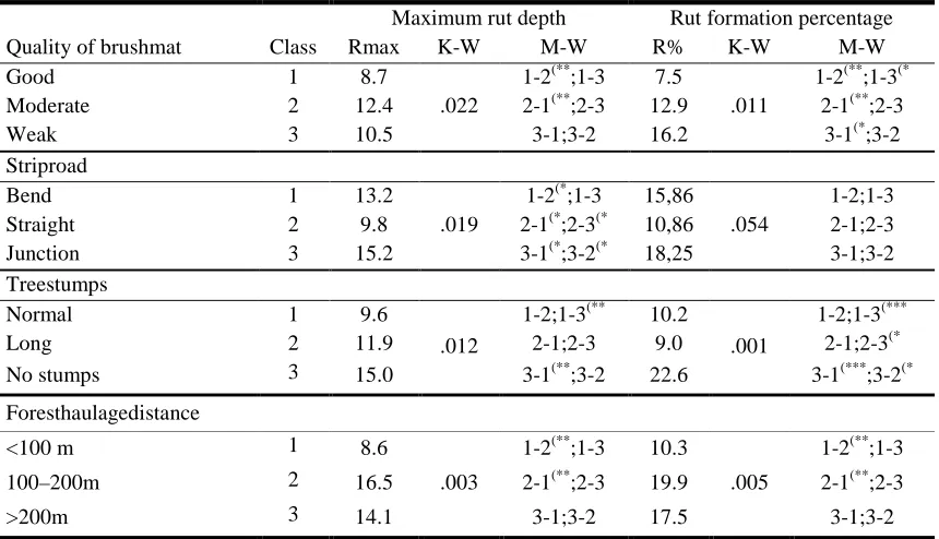
In this study, rut formation differences for classes of tree stumps, forest haulage distance, the quality of strip road networkand the quality of brush mat on strip road were

(10)

www.ijaems.com Page | 2049 Table.9: The effect of the quality of brush mat, the quality of strip road network, the length of stumps cut, and forest haulage

distance on the rut formation. Rmax = maximum rut depth, K-W = Kruskal-Wallis, M-W = Mann-Whitney, R% = rut formation percentage.(* =p < 0.05 is almost statistically meaningful,(** =p < 0.01 is statistically meaningful,(*** =p < 0.001

is statistically very meaningful variable.

Maximum rut depth Rut formation percentage Quality of brushmat Class Rmax K-W M-W R% K-W M-W

Good 1 8.7

.022

1-2(**;1-3 7.5

.011

1-2(**;1-3(* Moderate 2 12.4 2-1(**;2-3 12.9 2-1(**;2-3

Weak 3 10.5 3-1;3-2 16.2 3-1(*;3-2

Striproad

Bend 1 13.2

.019

1-2(*;1-3 15,86

.054

1-2;1-3

Straight 2 9.8 2-1(*;2-3(* 10,86 2-1;2-3

Junction 3 15.2 3-1(*;3-2(* 18,25 3-1;3-2

Treestumps

Normal 1 9.6

.012

1-2;1-3(** 10.2

.001

1-2;1-3(***

Long 2 11.9 2-1;2-3 9.0 2-1;2-3(*

No stumps 3 15.0 3-1(**;3-2 22.6 3-1(***;3-2(*

Foresthaulagedistance

<100 m 1 8.6

.003

1-2(**;1-3 10.3

.005

1-2(**;1-3

100–200m 2 16.5 2-1(**;2-3 19.9 2-1(**;2-3

>200m 3 14.1 3-1;3-2 17.5 3-1;3-2

Regression analysis of rut formation

Both variables of rut formation (i.e. rut formation percentage and maximum rut depth) correlated negatively with the depth to the groundwater table (Combination of ALS and field measurement), the height variation (ALS, 2×2 m) of stand, as well as the density of ALS pulse

reflecting from the vegetation. Both rut formation variables correlated positively with the thickness of peat layer and the value (ALS) describing the tree heightin the stand.Actually, there was a negative correlation between the values of potassium (GRL) and rut formation percentage (Table 10).

Table.10: The correlations (C) between the rut formation and independent variables of rut formation models in study plots (N). Rmax = maximum rut depth, R% = rut formation percentage.(* =p < 0.05 is almost statistically meaningful,(** =p < 0.01

is statistically meaningful,(*** =p < 0.001 is statistically very meaningful variable.

Thickness of peat layer

Height raster (2×2 m)

Depth to groundwater

table

Density of trees (2×2 m)

Height of stand (2×2 m)

Forest haulage distance

Potassium

Rmax R% Rmax R% Rmax R% Rmax R% Rmax R% Rmax R% Rmax R%

C .32 _(*** .40 _(*** -.34 _(** -.28 _(** -.44 _(*** -.33 _(*** _(*-.26 -.29 _(** .32 _(** .29 _(** .30 _(** .28 _(** -.20 ₍ -.29 _(*

N 115 115 96 96 113 113 85 85 96 96 115 115 54 54

Stepwise multiple regressions were conducted to predict rut formation and whether digital independent variables could be found by GIS, ALS or GRL for computational model. Actually, the regression analysis was conducted to evaluate how well useful variables of the Table 10 predicted maximum rut depth (Table 11). For example, at the final step of the analysis Depth to the groundwater table, the linear combination of Groundwater table and Height raster, entered into the regression equation, although it wasn’t statistically significantly related to maximum rut depth, p = .053.However, Potassium did not enter into the equation at steps of the analysis. The

multiple correlation coefficient was .73, indicating approximately .51% of the variance of the maximum rut depth could be accounted for by the model. Thus the regression equation for predicting maximum rut depth was: the maximum rut depth = 9.25×Dummy variable+ .12×Maximum rut depth + .03×Thickness of peat layer + -3.04×Depth to the groundwater table-10.05.

(11)

Infogain Publication (Infogainpublication.com statistically highly significant. Forest haulage and the depth to the groundwater table were

almost significant explanatory variables. When the thickness of peat layer and the forwarding distance grew, the maximum rut depth increased. In addition to this, when the depth to the groundwater table

maximum rut depth reduced. The depth to the groundwater table was partly digital independent variable provided by ALS data.

According to the analysis of variance, a model agreed to statistically very significant. The frequency distribut

Table.11: An explanatory model for t

y = a+ b1k1 + b2x1+ b3x2+ b4x3

where

y = maximum rut depth, cm

k1 = dummy variable: 0 = harwarder, 1

x1 = thickness of peat layer, cm

x2 = forest haulage distance, m

x3 = depth to the groundwater table, cm

a = constant

b1, b2, b3,b4 = coefficients of the variables

Variable Parameterestimate

a -10.047 b1 9.250

b2 0.121

b3 0.031

b4 -3.040

N R

95 .731

Sum of squares Regression 4866.911 Residual 4238.520 Total 9105.432

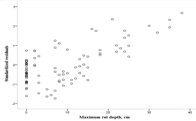
Fig.6: The distribution

Infogainpublication.com)

nt. Forest haulage distance water table were statistically natory variables. When the layer and the forwarding distance grew, In addition to this, e depth to the groundwater table increased, the educed. The depth to the groundwater table was partly digital independent variable

, a model agreed to requency distribution of

standardized residuals formed a little to the right of the entire panoply of distribution (Figure 6

Kolmogorov-Smirnov test, the residuals

normally distributed. The standard deviation of the residuals of the model was around zero on both sides when the maximum rut depth was less than 15 cm (Figure 7). However, with larger depth of ruts, the model givesthe higher values than realistic

depth. In this respect, unreliab observed in the graph of residuals

An explanatory model for the maximum rut depth of strip road network

= dummy variable: 0 = harwarder, 1 = two-machine system (i.e. harvester & forwarder)

= depth to the groundwater table, cm

= coefficients of the variables

Standard error Standardized

regression coefficient t-value

3.252 -3.089

1.690 0.472 5.474

0.029 0.306 4.212

0.015 0.156 2.046

1.553 -0.166 -1.958

R2 Adjusted R2 Meanerror of estimate

.535 .514 6.863

Degree of freedom Mean square F value

4 1216.728 25.836

90 47.095

94

The distribution of the standardized residuals of the regression model

ISSN : 2454-1311 formed a little to the right of the noply of distribution (Figure 6). According to the Smirnov test, the residuals were almost . The standard deviation of the was around zero on both sides h was less than 15 cm (Figure larger depth of ruts, the model givesthe values for the maximum rut unreliability of the model can be in the graph of residuals.

rut depth of strip road network.

ne system (i.e. harvester & forwarder)

p-value

.003 .000 .000 .044 .053

Meanerror of Kolmogorov- Smirnov .049 p value .000

(12)

International Journal of Advanced Engineering, Management and Science (IJAEMS) [Vol Infogain Publication (Infogainpublication.com

www.ijaems.com Fig.7: The residuals of the regression model of maximum rut depth

IV. DISCUSSION Study material and the reliability of results The number of plots for determination of conditionswas examined and selected by

effective sample size withthe formula of systematic sampling. For this purpose, it was aimed to select stands based on summertime harvesting. Nonetheless, t sampling frequency was determined a little denser there was only estimate which stands will be

harvest during summertime in the early planning stage the study. On the other hand, theaccuracy of spatial data sets and the size of raster for maps were

consideration in the design of study plot network. The density of study plot network was determined by the accuracy of potassium data (50×50 m), even though some of study material was more accurate. The length of study plot was established on 12 m, which, in fact, is a sample of the data in large-scale geographical dat

hand, in the small-scale data, the length is g diameter of raster. This feature could cause

errors for the study results. However, it can be assumed that the spatial autocorrelation reduce possible errors for instance in the variables of vegetation.

The data of harvesting results were collect stand had been harvested completely. Therefore results depict rut formation of the entire harvesting system (i.e. caused by both harvester and forwarder harwarder). The carrying capacity rating for harvesting machinery was conducted by the limit table

ground pressures (cf. Table 2), because the

were incomplete for the calculation of the nominal ground pressures exactly for harvesters and forwarders. Still, from the point of view of the study objective, it can be presumed that the nominal ground pressures of

machinery were classified enough accurately.

respect, results of rut formation and modelling work are reliable for consideration of practical forest operations.

of Advanced Engineering, Management and Science (IJAEMS) [Vol Infogainpublication.com)

The residuals of the regression model of maximum rut depth

material and the reliability of results

determination of the harvesting by calculating the the formula of systematic was aimed to select stands Nonetheless, the mined a little denser, as tands will be coming to planning stage of accuracy of spatial data of raster for maps were taken into in the design of study plot network. The was determined by the m), even though some e accurate. The length of study 12 m, which, in fact, is a sample geographical data. On the other is greater than the cause minor sample er, it can be assumed reduce possible errors for

were collected when the . Therefore the rut formation of the entire harvesting system (i.e. caused by both harvester and forwarder or The carrying capacity rating for harvesting machinery was conducted by the limit table of nominal Table 2), because the source data were incomplete for the calculation of the nominal ground d forwarders. Still, the point of view of the study objective, it can be nominal ground pressures of harvesting classified enough accurately. In this modelling work are forest operations.

Effects of harvesting conditions rut formation

The study results indicated that the carrying capacity classes of harvesting machinery (cf. T

the planning of wood harvesting

peat lands, since there were statistically highly significant differences between the categories

rut formation. When carrying capacity decreased or nominal ground pressures increased, rut formation gr The higher carrying capacity

caused by harvesters. Hence, the result und

is important to equip also a harvester so that it has a low nominal ground pressure and further higher carrying capacity class. The results showed that

haulage timber from harvesting site the carrying capacity class forwarders of the class 2 acceptable and unacceptable, current criteria of harvesting result study support the conclusions of

the reduction of nominal ground pressure ( capacity class of 3) is crucial in harvesting on peat lands (S

2008; Lamminen 2008; Kärhä &Poikela 2010; Kärhä et al. 2010; Lindeman 2010).

difference between the carrying capacity classes, the carrying capacity classes 1 and 2 were taken

analysis in order to examine reliab harvesting conditions and cutting It is not necessary to measure pressure of harvesting machinery

tools, if the carrying capacity classes of used in planning.

The thickness of peat layer

formation with so-called harvesting machines equipped with the weak carrying capacity (C

of Advanced Engineering, Management and Science (IJAEMS) [Vol-2, Issue-12, Dec- 2016] ISSN : 2454-1311

Page | 2051 The residuals of the regression model of maximum rut depth.

conditions and cutting results on

The study results indicated that the carrying capacity classes of harvesting machinery (cf. Table 2) are useful in arvesting operations of drained statistically highly significant the categories of carrying capacity in carrying capacity decreased or nominal ground pressures increased, rut formation grew. The higher carrying capacity also reduces rut formation Hence, the result underlines that it important to equip also a harvester so that it has a low nominal ground pressure and further higher carrying showed that it is impossible to from harvesting site with the forwarders of capacity class 1 during summer. The 2caused rut formation, both acceptable and unacceptable, if they were used under the harvesting results. The results of this conclusions of the previous studies that he reduction of nominal ground pressure (i.e. the carrying is crucial in successful wood lands (Sirén 1987; Airavaara et al. Kärhä &Poikela 2010; Kärhä et ). As there was significant carrying capacity classes, the 1 and 2 were taken for further to examine reliably the impact of cutting results on rut formation. It is not necessary to measure digital nominal ground of harvesting machinery using any laser scanning capacity classes of machinery are

(13)

Infogain Publication (Infogainpublication.com) ISSN : 2454-1311 thickness of peat layer was also the most powerful

independent variable in the regression model of maximum rut depth (cf. Model 1, Table 11). The results support the previous studies, in which the thickness of peat layer has been found to have an effect on rut formation (Kärhä &Poikela 2010; Kärhä et al. 2010; Lindeman 2010). In further analysis, the classes of thickness of peat layer was used to test the spatial data: Actually, there was no significant difference between the raster values of potassium (GRL) in four classes of the thickness of peat layer (the model by GTK), even though the mean values of the results were behaving consistently, i.e. the rut formation increased when the value of potassium reduced. Although the values of potassium and rut formation had statistically almost significant negative correlation, the correlation was lower than the correlation of alternative independent variables, so that it did not come to be selected to the model. This was harmful, because raster values of potassium (GRL) were digital and would have been readily available for a computational model.

In some study stands the terrain rose quite sharply, so the reflections of mineral soil from the edge of swamp or the spoil bank of ditches could consequently cause error sources for the intensity ofradiation by GRL (cf. Virtanen 1990; Virtanen &Vanne 2008). Due to this, especially on border bog, the radiation values of plots could be too high. The drainage also affected the intensity of radiation (Virtanen &Vanne 2008). Close to the ground the groundwater can prevent radiation altogether, in which case the observation imagesthe low radiation spot of thick peat layer. This is likely caused multicollinearityness between potassium, the thickness of peat layer, the depth to the groundwater table, and rut formation, even though it did not separately tested in the study. Actually, the separate variables with the maximum correlation come to select to the model instead of combined factor. This reasoning was supported by the observations of the carrying capacity classes 1 and 2, in which rut formation continued to increase,if groundwater table rose closer to the ground surface. Also, we have to remember that the digital potassium material was quite old: in some places around 40 years; this can also cause untrustworthiness for the study results related to the potassium data.During this period, for instance, the depth to the groundwater table, drainage situation, and trees in stand may have changed. On the basis of the above, it should be noted that there are some problems with the accuracy and reliability of data sources in the potassium data when the values of potassium is used in estimating rut formation in operational wood harvesting planning. On the other hand, the data is as the thickness of peat layer portraying the most comprehensive in Finland and could still be suited for planning models at the strategic level of wood

harvesting. Ala-Ilomäki (2005) has received similar results in his tests of an operational planning context. There was an indication of the impact of the depth to groundwater table on rut formation in the investigation by Lindeman (2010). The results of this study confirmed connection between the depth to the groundwater table and rut formation, when the wood harvesting machinery with the low carrying capacity (i.e. Classes of 1 and 2)are used. The depth to ground water table was also used as the independent variable in the regression model of the maximum rut depth(Model 1, Table 11). Utilization of the groundwater table level inplanning of wood harvesting operations can be justified also by spatial data. The results correspond to the results by Haavistoet al. (2011)and Uusitalo et al. (2012). The negative connection could be observed between the height of the ground surface and rut formation by using the values of ground surface model (ALS, 2×2 m). On the basis of the results of this study, it is suggested that the depth to the groundwater tableare combined withdigital height information asan useful operation, because the new combination variable explained rut formation better than just a ground surface model (2×2 m).When the groundwater data was connected to the height information, the model of maximum rut depth was statistically more significant and the stand selection was more reliable for summertime harvesting.Actually, infra-red beams can’t penetrate water in ditches. In future, it is possible to measure the depth to groundwater table using infra-green beam, which will replace manual measurements of groundwater table and provides digital information for computational models. The effect of the spatial variability of trees was tested by the raster values of tree volume (m3 ha-1) in the stand. Rut formation varied illogically between the classes of tree volume and there was no significant difference between the classes even several optional classifications were used. In the studies by Haavisto et al. (2011)and Uusitalo et al. (2012), the basal area of the stand was a better independent variable for modelling rut formation than the tree volume in stand. The weaker explanation ability of tree volume per hectare related to the basal area of stand may be the result ofcontrovert influences of internal variation of variables in the stand, which is further discussed in detail for computational models of operational planning in the next chapter.

(14)

www.ijaems.com Page | 2053 the density of tree volume and the other vegetation in the

stand, increases, the rut formation reduces. The increase in the initial tree volume in the stand as well as in the density of tree volume likely increases the volume of bearing capacity by the root system network of trees and the amount of logging residues for using reinforcement the strip roads, which factors together deduct rut formation (cf. Lamminen 2008).On the other hand, on the basis of the ALS data used in the study, rut formation increased when the height of trees in the stand grew. There was no statistically significant connection between the ALS values of the height and density of stand. Hardly, therefore, it can be concluded that the increase in the stand height reduces the tree density in the stand, and correspondingly affects rut formation. The increase in thestand height could be thought to increase the volume of timber haulaged to roadside in relation to the carrying potential of brush mat and therefore to have an increasing effect on rut formation.

In this study, the increase in logging residues, the quality of brush mat, the volume of bearing capacity of root system, the stand height and tree volume per hectare together had an increasing effect on the load size and the number of loads in forest haulage of timber. Therefore, the rut formation increased. When looking at the amount of logging residues remaining on strip road and setting out for strip roads separately, thus when they increased, the rut formation undoubtedly decreased. The amount of logging residues or the quality of brush mat have been shown to reduce rut formation also in the previous studies (Lamminen 2008; Kärhä &Poikela 2010; Kärhä et al. 2010; Lindeman 2010; Sirén et al.2013). According to results of this study, instead of detailed explanation of the above variables separately, itcould be successful to conduct the main component analysis to them. Unfortunately, this approach can’t be used in practical planning models or automated digitized planning systems at least in near future.

Combined effect of harvesting conditions were also established for several stands by the surface soil classification of general soil map (1:200,000), in which it was possible to distinguish rut formation that is affected by large-scale surface soil classes. Therefore, the accuracy of this material is sufficient for models of strategic wood harvesting planning at a regional level, such as Kokkila (2011) has proposed in her report. On the other hand, Salmi (2011) has underlined that, the basic soil map (1:20,000) is also difficult to use in the design of wood harvesting operations at the operational level. After careful analysis of rut formation at stand level, describing of harvesting conditions by geographical information succeeded and managed poorly. No cause-effect relationship was established. Although the harvesting conditions could be predicted so well that the

use of the spatial data sets can bepresented and justified, it should be suggested, that planning of harvesting operations must keep to make carefully by managers. It must keep in mind, that also cutting results affect significantly rut formation and cause the failure in several stands in summertime wood harvesting. For instance, the bends on strip road network increased rut formation, as it was the case in the several studies (Kärhä &Poikela 2010; Kärhä et al. 2010; Lindeman 2010). In this respect, professionalism of the operator of harvesting machinery is a great importance for the success of summer time wood harvesting on drained peat lands. On the other hand, requirements for the success of harvesting operations such as reinforcing a good brush mat will increase the time consumption and reduce the productivity ofwood harvesting. Therefore, work methods of skilful operators and the effective work models of harvesting should be figured out constantly every year to find, teach and learn the best working practices and job templates and hence to increase the cost-efficiency of wood harvesting on peat lands. For example, according to Ala-Ilomäki(2005), the slightly rear-loaded weight distribution is better than the front-loaded one. Palander et al. (2012b) have stated that machine operators are able to influence the load balance of 6-wheeled forwarder by front-butt loading in such a way that the rut formation reduces. According to their study, by using a forwarder loader, operators have the potential to impact on the weight distribution of the wheels and tracks and therefore rut formation.

Modelling of rut formation on drained peatlands Several stepwise multiple regressions were conducted to evaluate whichfield measurements were necessary to predict rut formation and whether they could be replaced by GIS-data for a computational model.In this study, the variables, which described the spatial variation in stands, were tried to include in the rut depth model. Finally, there was the thickness of peat layer, forwarding distance and the depth to the groundwater table as the independent variables in the best linear regression model of the maximum rut depth(Table 11). The thickness of peat layer and the depth to the groundwater table were in the regression models of rut depth by Lindeman (2010). On the basis of our correlation analysis, the density value of laser scanner reflected back from the vegetation would have been statistically significant variable, but on the basis of the additional findings measured, the model drawn up had a lower explanation degree than that of the model presented in this study (Table 11).However, the density value of laser scanning reflecting from the vegetation is reasonable to keep in mind, if such ALS materials exist in future.