95
Symbolic Simulation By Mesh Method of Effective
Branch Voltage Source
I. I. OKONKWO, P. I. OBI, K. J. OFFOR, & G. C CHIDOLUEAbstract – State variable are crucial to transient simulation initialization of electrical circuits. Other variable that are mathematical related to state variable may also be used to initialize transient response especially in symbolic simulation. In this paper we formulated and simulated electrical circuit transient symbolically using the transient mesh equation derived from branch effective voltage source. The result of the simulation agreed with the existing Matlab simpowersystem tool.
Index terms – transient simulation, state variable, symbolic simulation, electric circuit transient , voltage source, transient response and transient mesh equation.
1 INTRODUCTION
A single run of a conventional equation provides limited information about the behaviour of electrical circuit. It determines only how the circuit would behave for a single initial, input sequence and set of circuit parameter characterizing condition. Many cad tasks require more extensive information than can be obtained by a single simulation run. For example the formal verification of a design requires showing that the circuit will behave properly for all possible initial start sequences that will detect a given set of faults, clearly conventional simulation is of little use for such task. [1] Some of these tasks that cannot be solved effectively by conventional simulation have become tractable by extending the simulation to operate in a symbolic domain. Symbolic simulation involves introducing an expanded set of signal values and redefining the basic simulation functions to operate over this expanded set. This enables the simulator evaluate a range of operating conditions in a single run. By linearizing the circuits with lumped parameters at particular operating points and attempting only frequency domain analysis, the program can represent signal values as rational functions in the s ( continuous time ) or z (discrete time) domain and are generated as sums of the products of symbols which specify the parameters of circuits elements [2 – 4]. Symbolic formulation grows exponentially with circuit size and it limits the maximum analyzable circuit size and also makes more difficult, formula interpretation and its use in design automation application [5 – 8]. This is usually improved by using semisymbolic formulation, which is symbolic formulation with numerical equivalent of symbolic coefficient. Other methods of simplification include simplification before generation (SBG), simplification during generation SDG, and simplification after generation (SAG) [9 – 13]. Symbolic response formulation of electrical circuit may be classified broadly as modified nodal analysis (MNA), [14]. sparse tableau formulation and state variable formulation The state variable method were developed before the modified nodal analysis, it involves intensive mathematical process and has major limitation in the formulation of circuit equations.
Some of the limitations arise because the state variables are capacitor voltages and inductor currents [15]. The tableau formulation has a problem that the resulting matrices are always quite large and the sparse matrix solver is needed. Unfortunately, the structure of the matrix is such that coding these routine are complicated. MNA despite the fact that its formulated network equation is smaller than tableau method, it still has a problem of formulating matrices that are larger than that which would have been obtained by pure nodal formulation [16]. Though that mesh analysis may not be as powerful as the nodal analysis in power system because of a little bit of application complication in circuits with multiple branches in between two nodes, when power system is characterized with short line model, mesh analysis becomes a faster option especially when using laplace transient analysis. In this paper mesh symbolic method which uses transient branch effective voltage source for initialization is formulated.
2 S – DOMAIN MESH ANALYSIS
When simulation of electrical circuit involves investigation of parameter variation or the investigation of past response effect on the transient response of a circuit, clear structural representation of such parameter/quantity on the circuit response equation is necessary. For example the effect of fault angle on the branch current and in turn on the performance of a particular relay algorithm may require that the simulation equation explicitly express branch current as a function. In this paper a new mesh analytical method is introduced which may be used on linear or linearized RLC circuit and can be computer applicable and user friendly. The simplicity of the new transient mesh formulation lies in the fact that minimal mesh index is enough to formulate transient equation (1). Also standard method of building steady state mesh impedance bus is just needed to build the s – domain impedance bus while the branch source voltages are modified to its branch effective transient source voltages which comprises of the vector sum of the actual source voltage s – domain equivalent and the corresponding s – domain branch storage element induced voltage drop due to transient inception (2). When these are done a complete mesh circuit equation can easily be formulated. This method is called s – domain mesh method of branch effective voltage source in this paper. Simplicity, compactness and economy are the advantages of the newly formulated mesh equation.
( )
1 ) s ( E ) s ( I ) s (Z = e
where ___________________
• P. G. Scholars, in Dept. Of Elect. Engineering, Anambra State University, Uli. Nigeria* • Professor in Dept. Of Electrical Engineering,
96
( )
2(s) E E(s) (s)
Ee = + I
where also Z(s) is the Auxiliary impedance bus, s – domain equivalent of mesh impedance Ee(s) is the transient mesh
effective voltage source vector, E(s) is the actual steady state mesh voltage source vector transformed to s – domain, and EI(s) is the transient branch sum dc induced source voltage
mesh vector at the instant of transient inception due to the constitutive sum effect of branch storage elements on dc current flowing in these respective branches around various meshes at that instant of transient.
2.1 Transient Mesh Circuit Equation Formulation
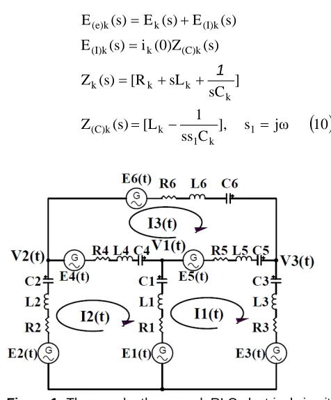
Consider circuit of fig 1, if Kirchhoff’s voltage law is applied round the various meshes then,
From mesh 1
( )
3 0 (t)dt I C 1 (t) I dt d L (t) I {R (t) E (t)]dt I (t) [I C 1 (t)] I (t) [I dt d L (t)] I (t) [I {R (t) E (t)]dt I (t) [I C 1 (t)] I (t) [I dt d L (t)] I (t) [I {R (t) E 1 3 1 3 1 3 3 3 1 5 3 1 5 3 1 5 5 2 1 1 2 1 1 2 1 1 1 = + + − − − + − + − − + − + − + − −∫
∫
∫
taking the laplace transform of equation (3) to get
( )
4 0 s (0) V s (0) V s (0) V (0)L I (0)]L I (0) [I (0)]L I (0) [I ] C 1 sL (s)][R I (s) [I ] C 1 sL (s)[R I ] C 1 sL (s)][R I (s) [I (s) E (s) E (s) E c5 c3 c1 3 1 5 3 1 1 2 1 5 5 5 3 1 1 1 1 1 1 1 1 2 1 5 3 1 = − − − + − + − + + + − − + + − + + − − + − but( )
5 , C s 1 (0)] I (0) [I (0) V C s 1 (0) I (0) V , C s 1 (0)] I (0) [I (0) V 5 1 3 1 c5 3 1 1 c3 1 1 2 1 c1 − = = − =Substituting equation (5) in (4) and simplifying to get
( )
6 ] C ss 1 (0)[L I ] C ss 1 (0)][L I (0) [I ] C ss 1 (0)][L I (0) [I (s) E (s) E (s) E (s) (s)Z I (s) (s)Z I (s)] Z (s) Z (s) (s)[Z I 3 1 3 1 5 1 5 3 1 1 1 1 2 1 5 3 1 5 3 1 2 5 3 1 1 − + − − + − − + + − = − − + +But from figure 1
( )
7 (0) I (0) i (0)], I (0) [I (0) i (0)], I (0) [I (0) i 1 3 3 1 5 2 1 1 − = − = − = ⇒( )
8 ] C ss 1 (0)[L i (s) E ]} C ss 1 (0)[L i (s) {E ] C ss 1 (0)[L i (s) E (s) (s)Z I (s) (s)Z I (s)] Z (s) Z (s) (s)[Z I 5 1 5 5 5 3 1 3 3 3 1 1 1 1 1 5 3 1 2 5 3 1 1 − + + − + − − + = − − + +simplifying to get
( )
9 (s) E (s) E (s) E (s) (s)Z I (s) (s)Z I (s)] Z (s) Z (s) (s)[Z I (e)5 (e)3 (e)1 5 3 1 2 5 3 1 1 + + = − − + + where( )
10
jω
s
],
C
ss
1
[L
(s)
Z
]
sC
sL
[R
(s)
Z
(s)
(0)Z
i
(s)
E
(s)
E
(s)
E
(s)
E
1 k 1 k (C)k k k k k (C)k k (I)k (I)k k (e)k=
−
=
+
+
=
=
+
=
1
Figure 1: Three node, three mesh RLC electrical circuit.
For mesh 2 similarly the Kirchhoff’s voltage law equation of mesh 2 may be obtained fig. (1) and simplified to get the following
( )
11 (s) E (s) E (s) E (s) (s)Z I (s) (s)Z I (s)] Z (s) Z (s) (s)[Z I (e)4 (e)2 (e)1 4 3 1 1 4 2 1 2 + + − = − − + +For mesh 3 similarly the Kirchhoff’s voltage law equation of mesh 3 may be obtained and simplified to get the following
( )
12 (s) E (s) E (s) E (s) (s)Z I (s) (s)Z I (s)] Z (s) Z (s) (s)[Z I (e)6 (e)5 (e)4 5 1 4 2 6 5 4 3 + − − = − − + +97
( )
13) s ( E ) s ( E ) s ( E ) s ( I ) s ( I ) s ( I ) s ( Z ) s ( Z ) s ( Z ) s ( Z ) s ( Z ) s ( Z ) s ( Z ) s ( Z ) s ( Z 3 ) eM ( 2 ) eM ( 1 ) eM ( 3 2 1 33 32 31 23 22 21 13 12 11 = Where
( )
) s ( Z ) s ( Z ) s ( Z ) s ( Z ) s ( Z ) s ( Z ) s ( Z ) s ( Z ) s ( Z 14 (s) Z (s) Z (s) Z ) s ( Z (s) Z (s) Z (s) Z ) s ( Z (s) Z (s) Z (s) Z ) s ( Z 4 32 23 5 31 13 1 21 12 6 5 4 33 4 2 1 22 5 3 1 11 − = = − = = − = = + + = + + = + + =( )
(s) E (s) E (s) E (s) E (s) E (s) E (s) E (s) E (s) E (s) E (s) E (s) E (e)6 (e)5 (e)4 (eM)3 (e)4 (e)2 (e)1 (eM)2 (e)5 (e)3 (e)1 (eM)1 + − − = + + − = + − = 15( )
16 (s) E (s) E K 1 k (e)k (eM)m∑
= = ⇒ WhereE(eM)m(s) → is the sum of all the effective source branch
voltages incident on the (m – th) mesh of the circuit
E(e)k(s) is the effective branch voltage source and it defined in
equation (10).
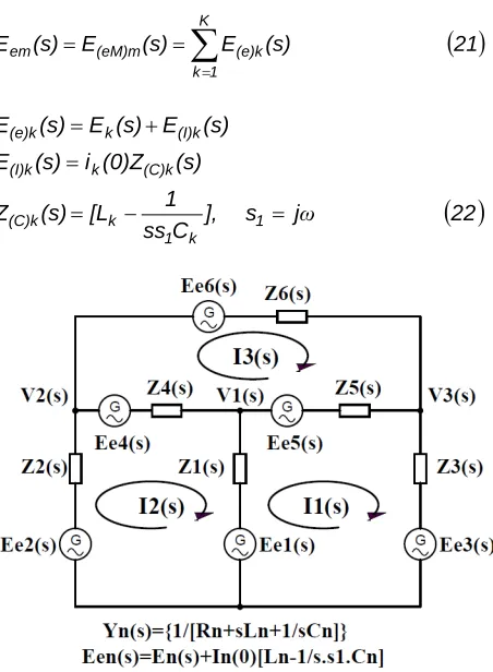
S – Domain Transient Equivalent Circuit Formulation
The derived equation (13) may be translated into circuit equivalent in s – domain as in fig. 2. This s – domain circuit of fig. 2 is corollary of fig. 1 with a modified branch source voltage of E(e)k(s) instead of Ek(t), equation (10) and all the
elements in the branches are transformed into their s – domain equivalent.
2.2 Generalized Matrix For Transient M–th Mesh Equation
Equation (13) may be used to generalize an equation for matrix form of mesh analysis of M – mesh electrical circuit, thus
( )
17 (s) E (s) E (s) E (s) I (s) I (s) I (s) Z (s) Z (s) Z (s) Z (s) Z (s) Z (s) Z (s) Z (s) Z (eM)m (eM)2 (eM)1 m 2 1 mm m2 m1 2m 22 21 1m 12 11 = Equation (17) may be treated as though it is standard steady state mesh equation but now in laplace frequency domain.
2.3 Generalized Compact Form for Transient M – th Mesh Equation
The generalized compact form of the equation 13 is thus as follows
( )
18
(s)
e
E
Z(s)I(s)
=
Where( )
19 (s) Z (s) Z (s) Z (s) Z (s) Z (s) Z (s) Z (s) Z (s) Z Z(s) mm m2 m1 2m 22 21 1m 12 11 = Z(s) is laplace frequency domain impedance bus, the admittance could be built from fig 2 using any standard method of building an impedance bus so far the branch impedances Zk(s) of the circuit is
evaluated as in equation (10c). In this paper it is called the s – domain auxiliary impedance bus.
Also
( )
20 , (s) E (s) E (s) E (s) E , (s) I (s) I (s) I I(s) m e 2 e e1 e m 2 1 = = I(s) and Ee(s) are the vector of mesh transient current and
transient mesh effective voltage source respectively, all in frequency domain.
( )
21 (s) E (s) E (s) E K 1 k (e)k (eM)m em∑
= = = ⇒( )
22 j s ], C ss 1 [L (s) Z (s) (0)Z i (s) E (s) E (s) E (s) E 1 k 1 k (C)k (C)k k (I)k (I)k k (e)k ω = − = = + =98
Definitions
ik(0) → is the steady state dc branch current at the instant of
transient inception in (k – th) branch of the circuit. Im(0) → is the steady state mesh dc current at the instant of
transient inception in (m – th) mesh of the circuit. Ek(s) → is the laplace transform of the (k – th) branch source
voltage.
Z(C)(s) → is the (k – th) branch laplace domain transient dc
driving point impedance due to the energy storing component in that branch. Z(C)(s) transforms the dc
current ik(0) flowing in the (k – th) branch to
transient dc induced source E(I)k(s) in that branch.
E(I)k(s) → is the transient dc induced source voltage in the (k
– th) branch at the instant of transient inception due to the constitutive effect of the branch transient impedance operator Z(C)k(s) on the dc current ik(0)
flowing in that branch at that instant.
E(e)k(s) → is the effective source voltage in the (k – th) branch
due to the net effect of source voltage and the induced dc source voltage at the instant of transient.
3 ANALYSIS PROCEDURES
3.1 Assignment Of Signs/Direction Of Source Voltage And Branch Current
Standard method of analysis in any standard electrical analysis textbook [17] is adopted, thus
• E(t) is assume positive if the mesh current orientation is such that it circulates by passing from the negative to positive ends of the voltage source. Note, in reality ac sign is the vectorial sense of voltage source as determined by its phasor. Nevertheless, the same source voltage which is seen as positive from a particular reference mesh would be seen as negative in another connected mesh whose mesh current rotation is in opposite direction.
• The magnitude and direction of the branch current will be set automatically by the following conditions,
( )
23
I I
ib = m + am
where ib is the branch current, Im is the reference mesh
current Im (‘m’ implies the reference frame at which the
analysis takes place) and Iam is the adjacent mesh Iam(‘am’
implies the adjacent mesh that share the branch ‘b’ with the reference frame ‘m’)
Also
( )
24
)
I
sign(I
)
sign(i
b=
m−
amWhere ib has the same sign/sense as Im, if
I
m>
I
amotherwise ib assume the same direction with Iam
Equations (23) and (24) are true for both time domain and frequency domain. Sign Of Induced Dc Source Voltage The sign of the induced dc source voltage may be determined by allowing it to be determined automatically by branch current sign as determined in equation (23).
3.2 Solution Procedure
1. Calculate the steady state branch current at transient inception.
2. transform all the branch impedances to their s – domain equivalents.
3. Transform all the branch voltage sources to s – domain (use laplace transformation).
4. Calculate the branch dc driving point impedance Z(c)k(s),
(10d) and use equation (10b) to calculate the branch dc induced branch source voltage.
5. Use equation (10a) to calculate effective transient voltage source.
6. Draw the s – domain equivalent of the RLC circuit by replacing the steady state circuit impedance with their s – domain equivalents, as they were calculated in step two. Also replace the branch steady state source voltage with their branch transient effective source voltage E(e)k(t) as
calculated in step 5.
7. From the s – domain transient equivalent circuit diagram, use any of the steady state method of formulating mesh equation to formulate s – domain transient mesh equation. It is worthy to note that formulated s – domain equivalent circuit is structured as a mere corollary of steady state circuit diagram. This is also true between the formulated transient mesh equation and the steady state mesh equation.
8. Form equation (17) solve for I(s) using Cramer’s rule. 9. Transform I(s) to time domain equivalent using laplace
inverse transform. Eg. in Matlab.
( )
25 )) s ( I ( ilap ) t ( I=
From this nodal voltages could easily be obtained at any instant.
4 TEST CIRCUIT
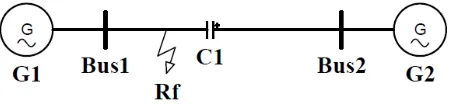
An earth faulted 100kV - double end fed, 70% series compensated 100km single transmission line was used for verification of the formulated s – domain transient mesh equation. In this analysis compensation beyond fault is adopted and fault position is assumed to be 70%.
Figure 3: earth faulted Single line with end line compensation.
Test Circuit Parameter Generator 1
E1 (t)=10x104sin(ωt), ZG1=(6+j40)Ω, S=1MVA
Generator 2
E2 (t)=0.8|E1|sin (ωt+450), ZG2=(4+j36)Ω, S=1MVA
Line Parameter
Rs=0.075 Ω/km, Ls=0.04875 H/km Gs=3.75*10-8 mho/km, Cs=8.0x10⁻⁹F/km Line length=100 km
99
4.1 Modeling
A lumped parameter was adopted as a model for the test circuit. It is assumed that compensation protection has not acted as such the compensation is of constant capacitance. More so, the model is characterized with constant parameter, shunt capacitance and shunt conductance of transmission line are shunt conductance is neglected. The equivalent circuit of the test circuit is represented below fig 4.
Figure 4: Single line equivalent circuit (short line model) for earth fault on end line compensation position.
5 TRANSIENT SIMULATIONS
5.1 Symbolic Simulation with Formulated Equation
In this paper the transient mesh currents are simulated by using the described formulation (s – domain mesh equation by method of branch equivalent transient voltage source). Analysis procedures of section 3 were used to calculate the s – domain rational functions of the mesh currents (17). The obtained s – domain rational functions were transformed to close form continuous time functions using laplace inverse transformation. Discretization of the close form continuous functions were done to plot the mesh current response graphs.
5.2 Simpower Simulation Of Test Circuit
To validate the formulated transient mesh equation, a simulation of the earth faulted line end series compensated single line transmission was performed using matlab simpowersystem software to obtain the circuit transient mesh current responses. Results were compared with the responses obtained from the simulations using the formulated transient mesh equation.
6 RESULTS
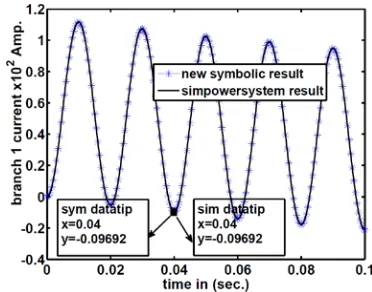
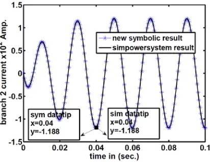
Transient mesh current response were simulated using the formulated mesh equation and also using simpower package, all simulation are done using Matlab 7.40 mathematical tool. Simulated responses by the methods for the earth faulted double end fed series compensated single line transmission are shown in fig 5 through fig 12. Mesh currents were taken for various simulating conditions. Simulating conditions included; zero initial condition, non – zero initial condition, high resistive (1000Ω) fault but at zero initial condition, and 1 sec. simulation. All simulations were done, except otherwise stated on 100km line at 70% fault position and 5Ω earth resistive fault. Sampling interval for the formulated equation simulation is 0.0005 sec, while that of the simpowersystem simulation is at 0.00005 sec. Evidence from data tip results of the simulated response graphs showed clearly excellent conformity between new mesh symbolic formulation and the simpowersystem simulation.
Test Circuit Simulated Mesh Voltage Response Graphs:
All graph are plotted except otherwise stated at the following conditions, 100 km Line, Compensation 70%, Fault Position=70%, And 5Ω Resistive Earth Fault.
Figure 5: Simulation Of Mesh Current Versus Time ; 0% Initial Condition.
Figure 6: Simulation Of Mesh Current Versus Time ; 0% Initial Condition.
100 Figure 8: Simulation of Mesh Current versus Time; Initial
Conditions, 0.015 Sec of Steady State Run.
Figure 10: Simulation Of Mesh Current Versus Time ; 0% Initial Condition, and 1000Ω Resistive Earth Fault.
Fig 6: Simulation Of Mesh Current Versus Time ; 0% Initial Condition, and 1000Ω Resistive Earth Fault.
Figure 11: Simulation Of Mesh Current Versus Time; 0% Initial Condition.
Figure 12: Simulation Of Mesh Current Versus Time ; 0% Initial Condition.
7 CONCLUSIONS
Simulation software has been formulated for transient simulation of RLC circuits initiated from steady state. The simulation software is especially useful for power circuits that are modeled with short line parameter. The result of the simulation of this new mesh symbolic software showed promising conformity with the existing simpowersystem package and has the advantage of being able to simulate complex initial conditions. This formulation may be modified easily for sub transient simulation.
REFERENCES:
[1] Randal E. Bryant” Symbolic Simulation—Techniques And Applications” Computer Science Department,. Paper 240. (1990).
[2] C.-J. Richard Shi And Xiang-Dong Tan “Compact Representation And Efficient Generation of S-Expanded Symbolic Network Functions For computer-Aided Analog Circuit Design” IEEE Transactions On Computer-Aided Design Of Integrated Circuits And Systems, Vol. 20, No. 7, July 2001.
101 [4] Gielen And W. Sansen, Symbolic Analysis For
Automated Design Of Analog Integrated Circuits. Norwell, Ma: Kluwer, 1991.
[5] A. Rodríguez-Vázquez, F.V. Fernández, J.L. Huertas And G. Gielen, “Symbolic Analysis Techniques And Applicaitons To Analog Design Automation”, IEEE Press, 1996.
[6] X. Wang And L. Hedrich, “Hierarchical Symbolic Analysis Of Analog Circuits Using Two-Port Networks”, 6th Wseas International Conference On Circuits, Systems, Electronics, Control & Signal Processing, Cairo, Egypt, 2007.
[7] P.Wambacq Et Al, “Efficient Symbolic Computation Of Approximated Small-Signal Characteristics”, IEEE J. Solid- State Circuits, Vol. 30, Pp. 327–330, Mar. 1995.
[8] Z. Kolka, D. Biolek, V. Biolková, M. Horák, Implementation Of Topological Circuit Reduction. In Proc Of Apccas 2010, Malaysia, 2010. Pp. 951-954.
[9] Tan Xd, “Compact Representation And Efficient Generation Of S-Expanded Symbolic Network Functions For Computer aided Analog Circuit Design”. IEEE Transaction On Computer-Aided Design Of Integrated Circuits And Systems,. Pp. 20, 2001.
[10] R. Sommer, T. Halfmann, And J. Broz, Automated Behavioral Modeling And Analytical Model-Order Reduction By Application Of Symbolic Circuit Analysis For Multi-Physical Systems, Simulation Modeling Practice And Theory, 16 Pp. 1024–1039. (2008).
[11] Q. Yu And C. Sechen, “A Unified Approach To The Approximate Symbolic Analysis Of Large Analog Integrated Circuits,” Ieee Trans. On Circuits And Systems – I: Fundamental Theory And Applications, Vol. 43, No. 8, Pp. 656–669, 1996. [12] P. Wambacq, R. Fern´Andez, G. E. Gielen, W.
Sansen, And A. Rodriguez- V´Zquez, “Efficient Symbolic Computation Of Approximated Small-Signal Characteristics,” IEEE J. Solid-State Circuit, Vol. 30, No. 3, Pp. 327–330, 1995.
[13] O. Guerra, E. Roca, F. V. Fern´Andez, And A. Rodr´Iguez-V´Azquez,, “Approximate Symbolic Analysis Of Hierarchically Decomposed Analog Circuits,” Analog Integrated Circuits And Signal Processing, Vol. 31, Pp. 131–145, 2002.
[14] C. W. Ho, Ruehli A, Brennan P. The Modified Nodal Approach To Network Analysis. Ieee Trans. Circuits Syst., P. 22. (1975).
[15] Ali Bekir Yildiz “Systematic Generation Of Network Functions For Linear Circuits Using Modified Nodal Approach” Scientific Research And Essays Vol. 6(4), Pp. 698-705, 18 February, 2011.
[16] R. Sommer, D. Ammermann, And E. Hennig “More Efficient Algorithms For Symbolic Network Analysis: Supernodes And Reduced Analysis, Analog Integrated Circuits And Signal Processing 3, 73 – 83 (1993).