A modified particle swarm optimization algorithm for parameter estimation of a biological system

R E S E A R C H

Open Access

A modified particle swarm optimization

algorithm for parameter estimation of a

biological system

Raziyeh Mosayebi

and Fariba Bahrami

Abstract

Background:Mathematical modeling has achieved a broad interest in the field of biology. These models represent

the associations among the metabolism of the biological phenomenon with some mathematical equations such that the observed time course profile of the biological data fits the model. However, the estimation of the unknown parameters of the model is a challenging task. Many algorithms have been developed for parameter estimation, but none of them is entirely capable of finding the best solution. The purpose of this paper is to develop a method for precise estimation of parameters of a biological model.

Methods:In this paper, a novel particle swarm optimization algorithm based on a decomposition technique is

developed. Then, its root mean square error is compared with simple particle swarm optimization, Iterative Unscented Kalman Filter and Simulated Annealing algorithms for two different simulation scenarios and a real data set related to the metabolism of CAD system.

Results:Our proposed algorithm results in 54.39% and 26.72% average reduction in root mean square error when

applied to the simulation and experimental data, respectively.

Conclusion:The results show that the metaheuristic approaches such as the proposed method are very wise

choices for finding the solution of nonlinear problems with many unknown parameters.

Keywords:Biological System Modeling, Iterative UKF, Particle Swarm Optimization, Simulated Annealing

Background

The parameter estimation of a biological model is a crucial step of a system description. These models are an approxi-mation of the real phenomenon and some of their param-eters do not have physical interpretation and their presence is to compensate the reductions and approxima-tions in the model. These approximaapproxima-tions often stem from the lack of our knowledge about the biological system.

The modelling of biochemical pathway is possible with the concurrent measurement of biochemicals. This is the result of latest developments in data acquisition technologies which provide us with abundance of time profiles of metabolites or proteins that can be used for mathematical modeling of biochemical networks [1].

The first step to mathematically model these phenom-ena is to specify a comprehensive framework that repre-sent the underlying structure and convey the thorough information. The second step is to choose a promising approach to find a global solution for the unknown pa-rameters of the model.

Frequently, the problem of biological parameter esti-mation are said to be NP hard, so they are multi-modal and ill conditioned i.e. there are more than one true so-lutions for the estimated parameters that fit the model and produce the time course information [2]. Many al-gorithms have been developed to address this problem. Among these algorithms, the gradient optimization methods often fail to reach the true solution due to its high sensitivity to initialization [3]. The heuristic algo-rithms however have been shown to be able to solve the NP hard problems and overcome the problem of multi-modality and achieve the global optimality [4].

* Correspondence:[email protected]

2_{CIPCE, School of Electrical and Computer Engineering, College of} Engineering, University of Tehran, Tehran, Iran

Full list of author information is available at the end of the article

Many researchers have investigated the problem of parameter estimation in biological systems. As the re-sults of their works, algorithms with promising out-comes have been emerged. EKF, IUKF, alternating regression, simulated annealing, firefly, and genetic algo-rithms are some example [5–10]. In [11], the author has developed an improved particle filter method for estima-tion of the parameters of an S-system, and shows the su-periority of this method over the ordinary particle filter algorithm from the accuracy and convergence rate point of view. Besides this method, Ding and et al. [12] have used a kalman filter based least square method for state estimation of canonical state space problem and a de-composition technique for enhancing the computational time. In [13], Moles and et al. have compared the global optimization methods for the problem of biochemical pathway modeling. In their paper, the authors have shown that the evolutionary algorithms such as meta-heuristic methods are the most proper choices for solving the NP hard problems and preventing from local solutions. Some other papers have employed the evolu-tionary algorithms. For example, in [14], the author de-veloped a hybrid firefly algorithm to estimate the parameter of a highly complex and nonlinear biological model. This method uses a neighborhood search by util-izing the evolutionary methods and compares its results in aspects of accuracy and computational time with the firefly and nelder-mead algorithms. In [15], the authors have demonstrated the capability of the evolutionary al-gorithms for estimation of the unknown parameters of a system in a reasonable amount of time. They proposed a parallel implementation of an enhanced Differential Evo-lution (DE) using Spark to reduce the computational time of the search process by including a selected local search and exploiting the available distributed resources. In [16], the author has modified the UKF algorithm to estimate the parameters of an E-coli system. The method is called Iterative UKF and is designed to pvent from the early saturation of the filter gain. As a re-sult the estimation error is decreased in comparison with the ordinary UKF algorithm.

One of the main problems of the parameter estima-tion of complex and highly nonlinear models is the cap-ability of the method to estimate the global solution. In these models, as the fitness function is non-convex, the number of the local solutions is large. This is the main reason of the algorithms such as the gradient base methods and optimal filtering that are unable to find the global solution, since these algorithms are highly sensitive to the initialization of the unknown parame-ters [3]. On the other hand, the evolutionary methods such as particle swarm optimization are powerful methods for exploring the search space in order not to stick in local solutions.

In this paper, a modified PSO algorithm is presented. In this method, a decomposition technique is employed so that the algorithm has higher ability for the exploitation technique near the final solution. The improvement of the exploitation technique results in minor movements of the particles near the global solution and prevents from larger jumps and deterioration of the value of fitness function. As a result, the method has less mean square error com-pare with the ordinary PSO algorithm.

The modified PSO algorithm is proposed for estima-tion of the parameters of a simulated biological model from a synthetic data [16]. This pathway generated data is modelled by a canonical model which is made by the S-system. Then, this algorithm is employed for real data of the E-coli system [15, 16]. The results of the algo-rithm are then compared with the IUKF, SA and PSO al-gorithms in Root Mean Square Error point of view. We have demonstrated that the novel PSO algorithm is ac-complished to estimate the true parameters and has less RMSE compare with the SA and IUKF and the ordinary PSO algorithm.

This paper is organized as follows. The mathematical modelling is defined in section II. The parameter estima-tion methods and the proposed technique are described in section III. The simulated and experimental results are presented in section IV and the paper is finally con-cluded in Section V.

Mathematical modelling Review stage

Consider a nonlinear dynamical model for a biological system as below:

_

x tð Þ ¼f x tð ð Þ;u tð Þ;wÞ ð1Þ

wherex∈ℝNis the metabolites,u∈ℝmis the concentra-tion vectors of biomolecules that is the vector of inde-pendent variables, and w∈ℝq is the parameter vector. The problem is to find a solution for the unknown pa-rameters that are best fitted to the model.

Different canonical modelling frameworks are available to describe a biological phenomenon. In this paper, among some frameworks such as Lotka-Volterra [17], S-systems [18], and cooperative and saturation models [19], the S-system is used to express the nonlinear model of eq. (1)

_

xi¼αi Y Nþm

j¼1 Y Nþm

k¼1;k≠j

xgij jx

gik k −βi

Y Nþm

j¼1 Y Nþm

k¼1;k≠j

xhij j x

hik

k ; i¼1;2;…;N;

ð2Þ

where αi> 0 and βi> 0 are rate coefficients andg and h

are kinetic orders. The number of dependent variables is

number of independent variables that are considered as inputs to the system.

Considering the eq. 2, we have x= [x1,…,xN]Tas the state vector, u= [xN+ 1,…,xN+m]T as the input vector

and w= [α1,…,αNβ1,…,βN,g11,…,gN, N+m,h11,…,hN, N

+m]Tas the parameter vector, whileq=N(2 + 2(N+m)) is

the largest number of the unknown parameters. Many algorithms have been developed to estimate the un-known parameters of such nonlinear equations. In sec-tion III, some of these methods are presented.

Methods

In order to compare the performance of the proposed method with another heuristic approach, the Simulated Anealling method is used. Moreover, for the further ana-lysis of heuristic methods, a non heuristic approach based on Unscented Kalman filter is applied. These methods be-sides the proposed algorithm are described in this section.

Iterative Kalman filter (IUKF)

The Unscented Kalman Filter (UKF) is a modified framework of the Kalman Filter for nonlinear modelling. In this filter, one or both the process and measurement equations might be nonlinear and the nonlinear kalman filter is required. The UKF algorithm employs the un-scented transform as a nonlinear transformation to com-pute the statistics of a random variable.

The UKF algorithm is briefly explained as follow: Consider the discrete state space model of eq. I:

x k½ þ1 ¼ F x kð ½ ;u k½ ;wÞ; ð3Þ

By the definition ofy[k] =x[k+ 1], k= 0, …, N−1, the above equation can be rewritten as the following nonlin-ear process equation:

y k½ ¼ F x kð ½ ;u k½ ;wÞ; ð4Þ

where x and u are the inputs,y is the output and w is the unknown parameter with dimension q that is to be estimated. To estimate the parameters, the following state space representation is defined as follows:

w k½ þ1 ¼w k½ þr k½

y k½ ¼ F x kð ½ ;u k½ ;w k½ Þ þe k½ ; ð5Þ

where the first model is the process equation, driven by

r as the process noise. The latter is the measurement equation driven by the input and the measurement noise

e. the UKF algorithm is able to estimate the parameterw

based on the following pseudo code:

1. Initialize the unknown parameter and the covari-ance matrix

ωb½ ¼0 E½ ω

Pω½ 0 ¼E ðω−ωb½ 0Þðω−ωb½ 0ÞT

h i _ð6Þ

2. Assuming the parameter vectorω with meanω and covariance Pω a set of 2q + 1 sigma vectors W are

ob-tained through the following equations

P−_{ω½ k} ¼Pω½k−1þRr½k−1W k½ jk−1

¼ ωb−½ k;bω−½ þk γqffiffiffiffiffiffiffiffiffiP−_{ω½ k};bω−½ k−γqffiffiffiffiffiffiffiffiffiP−_{ω½ k}

h i

; ð7Þ

where γ¼pffiffiffiffiffiffiffiffiffiffiffiqþλ, λ=ε2(q+ϗ)−q is a scaling param-eter, andðpffiffiffiffiffiffiffiffiffiffiffiffiffiffiffiffiffiffiffiffiffiffiðqþλÞPωÞirepresents the ith column of the matrix. The constant 10−4<ε< 1 controls the sigma points spread around ω. ϗ is also a scaling parameter, which is regularly fixed to 0 or 3−qand qis the dimen-sion of parameters [14].

3. The sigma points are transformed with the nonlin-ear processF

D½kjk−1 ¼ F x kð ½ ;u k½ ;W½kjk−1Þ ð8Þ

4. The mean and covariance of the transformed sigma point of step 3 are calculated as follows

db½ ¼k X2q_i¼0Wð Þ_imDi½kjk−1 ð9Þ

P_db;db½ ¼k X2q_i¼0Wð Þic Di½k kj −1−db½ k Di½k kj −1−db½ k T

þRe½ k;

h h

ð10Þ

WhereWð_imÞ¼Wð_icÞ¼ 1

2ðλþqÞ,Wð0mÞ¼W ðcÞ 0 ¼ðλþλqÞ. 5. The cross covariance matrix of the measurement and parameter vectors are calculated

P_ω;db½ ¼k X2q

i¼0W

c

ð Þ

i ½Wi½kjk−1−ωb−½ k Di½kjk−1−db½ k

T

h

ð11Þ

6. The kalman gain, parameters and the covariance matric is then updated

K½ ¼k P_ω;db½ kP−1

d

b;db½ k ð12Þ

ω

b½ ¼k Proj ωb½ þ Kk ½ k d k½ −db½ k

h i

ð13Þ

Pω½ ¼k P−_{ω½ k}−K½ kP_db;db½ Kk T½ k ð14Þ

To remedy this problem, the authors have developed the IUKF algorithm. In this algorithm, after applying the UKF algorithm, RMSE is calculated through the follow-ing equation

RMSE¼

ffiffiffiffiffiffiffiffiffiffiffiffiffiffiffiffiffiffiffiffiffiffiffiffiffiffiffiffiffiffiffiffiffiffiffiffiffiffi Xn−1

k¼0ðy k½ −yb½ kÞ 2 r

ð15Þ

wherey[k] is the true measurement and^y½k is the esti-mated output. If MSE is smaller than a threshold value

δE or the iteration number of the algorithm is large

enough the algorithm will stop, otherwise the UKF algo-rithm will be initialized with the final estimate of the pa-rameters and their covariance which produces better initial values for the UKF algorithm. If the difference of two consecutive RMSE is less than a threshold valueδR,

the covariance matrix resets to the first initial value pre-venting from small changes in covariance matrix.

Simulated annealing

SA algorithm is a meta-heuristic algorithm introduced by Scott Kirkpatrick and et al. [20]. This algorithm is based on heating and cooling of the materials, starting with a prior solution and improves it in a repetitive process to reach the optimized solution for the problem. It consists of an inner and outer loop. The inner loop displaces the last solution in a solution space with a local search and updates the obtained solution based on a probabilistic criterion. The outer loop decreases the temperature of the process consistently. This temperature affects the performance of the inner loop. In the beginning with high temperature, the algorithm performs well in searching the solution space and prevents from the local solution in non-convex problems. By decreasing the temperature, it demonstrates a good capability in exploration.

At the first iterations that the temperature is high, in the contrary to the non-proper value of the cost function, the probability of a bad solution in the inner loop is high. This property prevents the algorithm from convergence in local responses. In the last iterations of the outer loop with the loose of temperature, the probability of a bad solution is decreased and the most proper solution is chosen with high probability.

Particle swarm optimization

Particle Swarm Optimization, also called PSO, is a popula-tion based stochastic optimizapopula-tion method intruduced by Kennedy and Eberhart [21]. PSO simulates the activities of school of birds, swarms of insects or groups of fish, in which individuals are called particles and the population is named a swarm. In this method, a position P and a vel-ocity Vare assigned to each particle. These particles are scattered around in the search-space based on a few pro-cedures. The particles are scattered following their own

best known positionP*, in the search-space as well as the total swarm’s best known position P_g. The velocity of the

jth dimension of particle i in iteration t, is obtained as follow:

Vijð Þ ¼t W:Vijðt−1Þ þc1r1 Pijðt−1Þ−Pijðt−1Þ

þc2r2 Pgjðt−1Þ−Pijðt−1Þ

ð16Þ

Where W is the inertia weight and is normally in the range of 0.9–1.2 [22],c1andc2are constants that are set to 2, andr1andr2are randomly generated stochastic pa-rameters in the interval [0, 1].

The new position of theith particle is then updated by the following formula:

Pijð Þ ¼t Pijðt−1Þ þVijð Þt ð17Þ

The PSO algorithm is known as a fast simple method, suitable for non-convex NP-hard problems such as bio-logical pathway modelling. Despite its great performance in exploring the solution space, it has weakness in exploiting the optimal solution when reaching to its neighborhood. To cope with this deficiency, the re-searchers usually adopt some heuristics to the algorithm or hybridize it with some other methods. In this paper, a novel heuristic is embedded in the PSO algorithm to im-prove its exploiting capabilities. Here, we apply a decom-position technique in a sequential platform with the canonical PSO. The proposed algorithm, named as DPSO, has a two-phase structure. The first phase is a standard PSO, where the algorithm finds a solution in the neighborhood of the optimal one, known as the Global-Best. In order to enhance the capability of the first phase in reaching near the optimal solution as close as possible, the inertia weight in the eq. (16) is linearly reduced in each iteration of the PSO algorithm, ending with a final value equal to 0.1. Using this technique pro-vides the algorithm with more precision in the final iter-ations, when the particles are in the neighbor of the best solution. The second phase, utilizes a decomposition technique as following pseudo-code:

Fori= 1: Iteration Number For j = 1:Param_Number

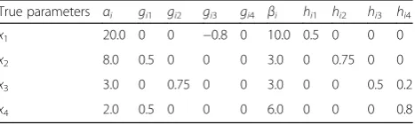
Table 1The chosen Parameters of the simulated S-system

True parameters αi gi1 gi2 gi3 gi4 βi hi1 hi2 hi3 hi4

x1 20.0 0 0 −0.8 0 10.0 0.5 0 0 0

x2 8.0 0.5 0 0 0 3.0 0 0.75 0 0

x3 3.0 0 0.75 0 0 3.0 0 0 0.5 0.2

– Relocate the position of all the particles as the global-best

– Scatter the particles in thejth dimension in the neighbor of the global-best

– Find the optimal value of thejth dimension using the PSO algorithm

– Update the global-best

endfor. endfor.

As described in the above pseudo-code, the second phase of the algorithm has an inner loop where it tries to find the optimal value of all the decision variables, considering the values of the others as constant values, using the canonical PSO. In the sec-ond phase, we needed to be more precise in our searching method. So, we concentrated the ability of the PSO algorithm from a multi-dimensional search space to a single-dimension exploitation: by decom-posing the problem into each decision variable, the PSO was able to search the optimal value of each decision variable near the vicinity of the best found solution at hand, while considering other decision variables as fixed values. This searching technique is repeated for all decision variables. In the outer loop, the whole procedure is repeated to insure evading from a local solution. Using this technique allows

the method to exploit the optimal solution with higher levels of accuracy, resulting in a reliable high quality solution.

Results Simulations

In this section, we demonstrate the capability of the modified PSO algorithm with two synthetic simulations. In the first simulation, no additive noise has been assumed. In the second simulation, additive white Gaussian noise with SNR = 20 is considered. The data are generated through the following model:

_

x1¼α1xg312x g15

5 −β1x h11

1

_

x2¼α2xg121−β2x h22

2

_ x3¼α3x

g32

2 −β3xh333xh434

_

x4¼α4xg141−β4x h44

4

ð18Þ

and the parameters are as follows:

ω¼ ½α1;α2;α3;α4;β1;β2;β3;β4;g13;g15;g21;g32;g41;

h11;h22;h33;h34;h44;

ð19Þ

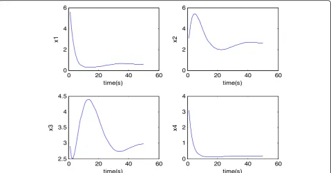
Table1shows the chosen parameters of the above model. Four random initial values are generated to produce the four synthetic metabolisms. The time profiles of

0 20 40 60

0 2 4 6

time(s)

x1

0 20 40 60

0 2 4 6

x2

time(s)

0 20 40 60

2.5 3 3.5 4 4.5

x3

time(s)

0 20 40 60

0 1 2 3 4

time(s)

x4

Fig. 1time profile of the four synthetic states: Four random initial values are generated to produce the four synthetic metabolisms according to

these four synthetic states are obtained from eq. (18) and shown in Fig.1.

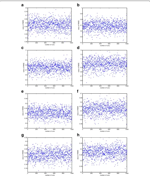
Tables 2 through 5 depict the results obtained from IUKF, SA, PSO and the proposed DPSO algorithms. In these tables, the average of estimated parameters and the corresponding average RMSE for each algo-rithm in 1000 simulations are presented. As it is ob-vious from the tables, DPSO algorithm has higher capabilty for estimating the unknown parameters in both simulation scenarios. The RMSE of the proposed method is less than the other three algorithms. These simulations demonstrate the enhancement of the ex-ploitation phase in the PSO algorithm employing the proposed technique compared with the ordinary PSO and also the capability of the method for estimation of more precise parameters compared with the IUKF and SA algorithms. Figure 2 illustrates the value of RMSEs of noise free and noisy scenarios in each 1000 simulation runs for each algorithm in Tables 2, 3, 4 and 5.

The mean percentage improvement of DPSO algo-rithms over SA, IUKF and PSO methods is 60.06% and 48.72% with respect to noise free and noisy scenarios.

Real data

In order to compare the performance of the algorithms in an experimental scenario, a real dataset is utilized from the Cad system. The Cad system is one of the conditional stress response modules in E. coli, which is induced only at low pH and a lysine-rich environment [23, 24]. The following S-system can be used to model this phenomenon

d CadA½

dt ¼α1½CadBA

g12−β

1½CadA h11

d CadBA½

dt ¼α2½Lys

g24½_Hþg25−β

2½CadBA h22

d Cadav½

dt ¼α3½CadA

g31½_Cadavg33½_Lysg34

d Lys½

dt ¼−β4½CadA

h31½_Cadavh33½_Lysh34

ð20Þ

The description and the parameters of the model have obtained from [16]. The parameters of this system have been estimated by the above mentioned methods. Then, these parameters will be used to generate the time profiles of the states of the Cad system in eq. (20). To compare the results of the algorithms, the RMSE is calculated as the error of the generated time profiles and the real Table 2The estimated parameters of two simulations for IUKF algorithm

True parameters αi gi1 gi2 gi3 gi4 βi hi1 hi2 hi3 hi4 RMSE

IUKF noise free measurement 0.5698

x1 20.4897 0 0 −0.3092 0 10.488 0.9954 0 0 0

x2 7.5180 1.5027 0 0 0 3.4884 0 1.7552 0 0

x3 3.4989 0 1.7556 0 0 2.4842 0 0 1.5019 0.7053

x4 2.4902 0.9887 0 0 0 6.4926 0 0 0 1.294

IUKF noisy measurement with SNR 20 0.6853

x1 19.6459 0 0 −0.1437 0 9.643 1.6490 0 0 0

x2 9.1521 1.1415 0 0 0 3.6681 0 1.4249 0 0

x3 3.6506 0 1.8956 0 0 3.6517 0 0 1.1638 0.8546

x4 2.6518 1.6585 0 0 0 7.6445 0 0 0 1.4447

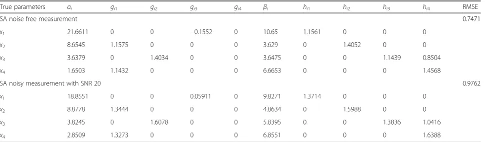
Table 3The estimated parameters of two simulations for SA algorithm

True parameters αi gi1 gi2 gi3 gi4 βi hi1 hi2 hi3 hi4 RMSE

SA noise free measurement 0.7471

x1 21.6611 0 0 −0.1552 0 10.65 1.1561 0 0 0

x2 8.6545 1.1575 0 0 0 3.629 0 1.4052 0 0

x3 3.6379 0 1.4034 0 0 3.6475 0 0 1.1439 0.8504

x4 1.6503 1.1432 0 0 0 6.6653 0 0 0 1.4568

SA noisy measurement with SNR 20 0.9762

x1 18.8551 0 0 0.05911 0 9.8271 1.3714 0 0 0

x2 8.8778 1.3444 0 0 0 4.8634 0 1.5988 0 0

x3 3.8245 0 1.6078 0 0 5.8395 0 0 1.3836 1.0416

datasets obtained by the measurements. Table6shows the resultant RMSEs.

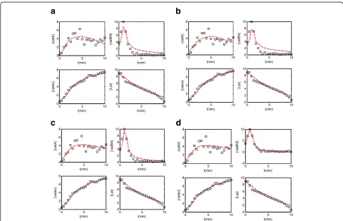
The generated time profiles obtained by the estimated parameters along with the true time profiles are depicted in Fig.3.

The proposed decomposition technique is applied on the ordinary PSO to have smaller movements near the global solution and prevent from larger jumps that de-teriorate the results. Therefore, as it is explained earlier, the DPSO algorithm has higher capability in exploitation step compared with the ordinary PSO algorithm. In the real dataset experiment, the RMSE of DPSO algorithm is 0.741 revealing the capability of the proposed method in comparison to IUKF and SA and PSO algorithms. For this real data experiment, the percentage improvement of DPSO algorithm over SA, IUKF and PSO methods is 29.36%, 33.78%, 17.02%, respectively.

Discussion

Four different algorithms have been discussed in this paper. IUKF has an analytical approach and it pro-vides the solution under the mathematics of kalman

filter. However, the heuristic approaches are very popular in the literature for the nonlinear problems with large number of parameters. Therefore, two metaheuristic approaches are considered besides IUKF. SA and PSO algorithms are two powerfull methods for finding the best solution in NP hard problems. The proposed DPSO algorithm is developed to have higher capability in exploitation step. As a re-sult this algorithm has less RMSE compared with the other three algorithm due to smaller jumps near the global solution. The results show the superiority of DPSO algorithms over the other three methods in RMSE point of view.

In simulations, a model with 17 parameters is consid-ered and two scenarios with different SNR have been ana-lysed. RMSE is computed with the estimated and the true parameters. The RMSE of DPSO is less than the other three algorithms as it is expected.

In real experiment scenario the data of CAD system is used to estimate the paramters of an assumed model for the time profile of the involved metabolisms. The model is similar to the one in simulation scenarios and the parameters are estimated. The DPSO method has Table 4The estimated parameters of two simulations for the PSO algorithm

True parameters αi gi1 gi2 gi3 gi4 βi hi1 hi2 hi3 hi4 RMSE

PSO noise free measurement 0.4040

x1 20.3569 0 0 −0.4444 0 10.3510 0.8602 0 0 0

x2 8.3541 0.858 0 0 0 3.3464 0 1.1024 0 0

x3 3.3513 0 1.1049 0 0 3.3478 0 0 0.8554 0.5437

x4 2.3560 0.8419 0 0 0 6.3490 0 0 0 1.148

PSO noisy measurement with SNR 20 0.5160

x1 16.0762 0 0 −0.3411 0 7.4571 0.9537 0 0 0

x2 8.4461 1.9448 0 0 0 3.4396 0 1.1908 0 0

x3 1.453 0 1.1971 0 0 3.4558 0 0 0.9496 0.6451

x4 2.4434 0.9482 0 0 0 8.4386 0 0 0 1.2565

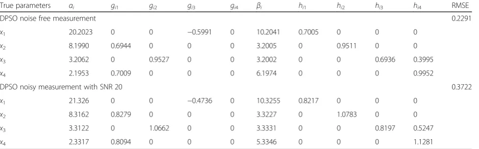
Table 5The estimated parameters of two simulations for the DPSO algorithm

True parameters αi gi1 gi2 gi3 gi4 βi hi1 hi2 hi3 hi4 RMSE

DPSO noise free measurement 0.2291

x1 20.2023 0 0 −0.5991 0 10.2041 0.7005 0 0 0

x2 8.1990 0.6944 0 0 0 3.2005 0 0.9511 0 0

x3 3.2062 0 0.9527 0 0 3.2002 0 0 0.6936 0.3995

x4 2.1953 0.7009 0 0 0 6.1974 0 0 0 0.9952

DPSO noisy measurement with SNR 20 0.3722

x1 21.326 0 0 −0.4736 0 10.3255 0.8217 0 0 0

x2 8.3162 0.8279 0 0 0 3.3227 0 1.0783 0 0

x3 3.3122 0 1.0662 0 0 3.3331 0 0 0.8197 0.5247

less RMSE between the true data and the data obtained from the model with the estimated parametrs. This ac-curacy is obtained as a result of more running time

compared with the PSO and SA algorithms. However, this time is not a significant problem because this methods are offline and a model is estimated to be used

0 200 400 600 800 1000

0.35 0.4 0.45 0.5 0.55 0.6 0.65 0.7 0.75 0.8

number of runs

E S M R f o e ul a v

0 200 400 600 800 1000

0.4 0.5 0.6 0.7 0.8 0.9 1

number of runs

E S M R f o e ul a v

0 200 400 600 800 1000

0.4 0.5 0.6 0.7 0.8 0.9 1 1.1

number of runs

E S M R f o e ul a v

0 200 400 600 800 1000

0.5 0.6 0.7 0.8 0.9 1 1.1 1.2 1.3

number of runs

E S M R f o e ul a v

0 200 400 600 800 1000

0.25 0.3 0.35 0.4 0.45 0.5 0.55 0.6

number of runs

E S M R f o e ul a v

0 200 400 600 800 1000

0.35 0.4 0.45 0.5 0.55 0.6 0.65 0.7

number of runs

E S M R f o e ul a v

0 200 400 600 800 1000

0.16 0.18 0.2 0.22 0.24 0.26 0.28 0.3 0.32

number of runs

E S M R f o e ul a v

0 200 400 600 800 1000

0.2 0.25 0.3 0.35 0.4 0.45 0.5

number of runs

E S M R f o e ul a v

a

b

c

d

e

f

g

h

Fig. 2the RMSEs of 1000 simulation runs for noise free and noisy scenarios. The figures in left column represent the noise free scenario inaIUKF,

for further analysis. The running time of each algorithm is 343, 305, 287 and 416 s for IUKF, SA, PSO and DPSO algorithms, respectively.

Conclusion

In this paper, a PSO based algorithm is suggested to esti-mate the unknown parameters of the nonlinear biological models. The proposed method is compared against IUKF, SA and the ordinary PSO algorithm. The results show the superiority of the DPSO algorithm compared with the other three methods. The results of the simulation and ex-perimental scenarios reveal the capability of the proposed algorithm for estimation of the unknown parameters of a nonlinear biological system.

Acknowledgments

RM is grateful to Dr. Mehrdad Gholami-Shahbandi for his comments on metaheuristic approaches and for English proofreading of the paper.

Funding

This research is funded by no institute or organization.

Availability of data and materials Please contact author for data requests.

Authors’contributions

RM is the main author of the paper and FB is the advising professor and helped to draft the manuscript. Both authors read and approved the final manuscript.

Authors’information

Raziyeh Mosayebireceived her Bs.c and Ms.c. degree in Electrical Engineering from Amirkabir University of Technoogy, Tehran, Iran in 2011 and 2013, respectively. She then joined the biomedical Engineering department at University of Tehran in 2014 as a Ph.D. student. She is currently working on signal processing tools for fusion of EEG and fMRI data. Her main focus is on data decomposition and factorization methods. Fariba Bahramiis an associate professor at the University of Tehran, School of Electrical and Computer Engineering, Department of Biomedical Engineering. She received her B.S. and M.S. degrees in Communication Engineering from Technical University of Isfahan, Isfahan, Iran, in 1985 and 1988, respectively, and her Ph.D. degree from the University of Tehran at 1998 in Biomedical Engineering. She accomplished a part of her PhD research at Technical University of Munich, in Munich, Germany from 1994 to

0 5 10

0 2 4 6 8 t(min) ] A d a c[

0 5 10

0 2 4 6 8 10 t(min) [c a d B A ]

0 5 10

0 2 4 6 8 t(min) ]v a d a c[

0 5 10

0 2 4 6 8 10 t(min) [L ys ]

0 5 10

0 2 4 6 8 t(min) ] A d a c[

0 5 10

0 2 4 6 8 10 t(min) [c a d B A ]

0 5 10

0 2 4 6 8 t(min) ]v a d a c[

0 5 10

0 2 4 6 8 10 t(min) [L ys ]

0 5 10

0 2 4 6 8 t(min) ] A d a c[

0 5 10

0 2 4 6 8 10 t(min) [c a d B A ]

0 5 10

0 2 4 6 8 t(min) ]v a d a c[

0 5 10

0 2 4 6 8 10 t(min) [L ys ]

0 5 10

0 2 4 6 8 t(min) ] A d a c[

0 5 10

-5 0 5 10 t(min) [c a d B A ]

0 5 10

0 2 4 6 8 t(min) ]v a d a c[

0 5 10

0 2 4 6 8 10 t(min) [L ys ]

a

b

c

d

Fig. 3: the estimated time profile of the true data set with the three algorithms:aIUKF,bSA,cPSO,dDPSO: the red color shows the estimated

time course and the squares represent the true data points. DPSO algorithm has less RMSE compared with the other algorithms and it can be inferred from the figure. The estimated time profile of DPSO method follows the variations of the true values more precisely

Table 6The RMSE of the three algorithms in real data experiment

Algorithms IUKF SA PSO DPSO

1997 under a stipendium from DAAD, Germany. She was the vice president of Iranian Society of Biomedical Engineering (ISBME) from 2009 to 2015 and she has been an editorial board member of Iranian Journal of Biomedical Engineering since 2007. Her field of interests are biological system modeling, computational and cognitive neuroscience, human motor control and neurorehabilitation. She is a member of IEEE, EMB Society.

Ethics approval and consent to participate Not Applicable.

Consent for publication Not applicable.

Competing interests

The authors declare that they have no competing interests.

Publisher’s Note

Springer Nature remains neutral with regard to jurisdictional claims in published maps and institutional affiliations.

Author details

1_{School of Electrical and computer Engineering, College of Engineering,} University of Tehran, Tehran, Iran.2CIPCE, School of Electrical and Computer Engineering, College of Engineering, University of Tehran, Tehran, Iran.

Received: 27 May 2018 Accepted: 15 August 2018

References

1. Harrigan GG, Goodacre R, eds. Metabolic profiling: its role in biomarker discovery and gene function analysis. Springer Science & Business Media, 2012.

2. Gu X. A multi-state optimization framework for parameter estimation in

biological systems. IEEE/ACM Trans Comput Biol Bioinform. 2016;13(3): 472–82.

3. Friedl G, Kuczmann M. Population and gradient based optimization techniques, a theoretical overview. Acta Technica Jaurinensis. 2014;7(4):378–87. 4. Doerner KF, Maniezzo V. Metaheuristic search techniques for multi-objective and stochastic problems: a history of the inventions of Walter J. Gutjahr in the past 22 years. CEJOR. 2018;26(2):331–56.

5. Meskin N, et al. Parameter estimation of biological phenomena modeled by

s-systems: An extended kalman filter approach. Decision and Control and European Control Conference (CDC-ECC), 2011 50th IEEE Conference on. IEEE, 2011.

6. Chou I-C, Martens H, Voit EO. Parameter estimation in biochemical systems models with alternating regression. Theor Biol Med Model. 2006;3:25. 7. Daniels BC, Nemenman I. Efficient inference of parsimonious

phenomenological models of cellular dynamics using S-systems and alternating regression. PLoS One. 2015;10(3):e0119821.

8. Wang C, Zhang L. Comparison of parameters estimation methods based on

the systems biology model of breast cancer. Progress in Informatics and Computing (PIC), 2015 IEEE International Conference on. IEEE, 2015.

9. Gonzalez OR, et al. Parameter estimation using simulated annealing for

S-system models of biochemical networks. Bioinformatics. 2006;23(4): 480–6.

10. Chou I-C, Voit EO. Recent developments in parameter estimation and structure identification of biochemical and genomic systems. Math Biosci. 2009;219:57_–83.

11. Mansouri MM, et al. State and parameter estimation for nonlinear biological phenomena modeled by S-systems. Digital Signal Process. 2014;28:1–17. 12. Ding F, Liu X, Ma X. Kalman state filtering based least squares iterative

parameter estimation for observer canonical state space systems using decomposition. J Comput Appl Math. 2016;301:135–43.

13. Moles CG, Mendes P, Banga JR. Parameter estimation in biochemical pathways: a comparison of global optimization methods. Genome Res. 2003;13:2467_–74.

14. Abdullah A, et al. An evolutionary firefly algorithm for the estimation of nonlinear biological model parameters. PLoS One. 2013;8(3):e56310. 15. Teijeiro D, et al. A cloud-based enhanced differential evolution algorithm for

parameter estimation problems in computational systems biology. Clust Comput. 2017;20(3):1937–50.

16. Meskin N, et al. Parameter estimation of biological phenomena: an unscented Kalman filter approach. IEEE/ACM Trans Comput Biol Bioinform. 2013;10:2.

17. Skvortsov A, Ristic B, Kamenev A. Predicting population extinction from early observations of the Lotka–Volterra system. Appl Math Comput. 2018; 320:371_–9.

18. Meskin N, Nounou H, Nounou M, Datta A, Dougherty ER. Parameter

estimation of biological phenomena modeled by S-systems: an extended Kalman filter approach: Proc IEEE 50th Decision and Control and European Control Conf (CDC-ECC); 2011. p. 4424_–9.

19. Sorribas B, Hernndez-Bermejo EV, Alves R. Cooperativity and saturation in biochemical networks: a Saturable formalism using Taylor series approximations. Biotechnol Bioeng. 2007;97(5):1259–77.

20. Kirkpatrick S, Daniel Gelatt C, Vecchi MP. Optimization by simulated annealing. Science. 1983;220(4598):671–80.

21. Eberhart R, Kennedy J. A new optimizer using particle swarm theory. In: Micro machine and human science, 1995. MHS’95, Proceedings of the sixth international symposium on: IEEE; 1995.

22. Shi Y, Eberhart RC. A modified particle swarm optimizer: Proc. of IEEE World Conf. on Computation Intelligence; 1998. p. 69_–73.

23. Küper C, Jung K. CadC-mediated activation of the cadBA promoter in Escherichia coli. J Mol Microbiol Biotechnol. 2005;10(1):26_–9. 24. Fritz G, Koller C, Burdack K, Tetsch L, Haneburger I, Jung K, Gerland U.