from Censored Samples in Burr Type X Distribution
R.R.L. Kantam
Department of Statistics, Acharya Nagarjuna University Nagarjunanagar-522510, Guntur-Andhra Pradesh, India [email protected]
M.S. Ravikumar
Department of Community Medicine
Konaseema Institute of Medical Sciences & Research Foundation/ General Hospital, Amalapuram-533201, Andhra Pradesh, India [email protected]
Abstract
The two parameter Burr type X distribution is considered and its scale parameter is estimated from a censored sample using the classical maximum likelihood method. The estimating equations are modified to get simpler and efficient estimators. Two methods of modification are suggested. The small sample efficiencies are presented.
Keywords: MLE, Censored Samples, Order Statistics, Asymptotic Variance.
1. Introduction
In reliability studies exponential distribution is the central model for the study of any phenomenon through a probabilistic approach. Extension of this model into two different directions yields two popular models called the Weibull distribution and the gamma distribution. Between these two, the Weibull distribution is more frequently applied model in any practical situation concerning reliability studies. Both Weibull and gamma distributions involve a shape parameter, in the sense that the shape of the frequency curve of these models changes according as the change in the values of the shape parameters. In particular, for the Weibull distribution its shape parameter classifies it into an Increasing Failure Rate (IFR) model or a Decreasing Failure Rate (DFR) model or Constant Failure Rate (CFR) model (the well known exponential model) as its special cases. The natural phenomenon in reliability is “The aging concept” – indicated by increasing instantaneous failure probability with age of the product. A specific case of Weibull distribution exhibiting aging effect with an integer valued shape parameter is known as “The Rayleigh distribution”. Its cumulative distribution function (CDF), probability density function (PDF) and hazard function are given by
( ) (1.1)
( ) (1.2)
( ) (1.3)
If F(x) is the cumulative distribution function of a positive valued random variable, then
a parallel system of k- components whose life times are independently and identically
distributed random variables, each with a common CDF – F(x) if k is an integer.
Exploring this concept to non integer values of k also, many researchers in the recent past
made extensive studies on models of the type [ ( )] generated by a basic well known
model F(x). Such new models are named as exponentiated models by some authors and
generalised models by some authors. For instance if the basic F(x) is exponential,
[ ( )] is named as generalised exponential (Gupta & Kundu- 1999), if F(x) is Weibull,
[ ( )] is named as exponentiated Weibull (Mudholkar and Srivastava – 1993). Banking on this notion, generalised Rayleigh distribution was studied by Raqab and Kundu (2006), as a process of revisit to Burr type X distribution. Its cumulative distribution function (CDF), probability density function (PDF) and hazard function are given by
( ) ( ) ; x>0, k>0 (1.4)
( ) ( ) ; x>0, k>0 (1.5)
( ) ( )( )
( ) (1.6)
Burr (1942) has suggested a number of forms of cumulative distribution functions that might be useful in modeling various practical situations. In all, he suggested twelve models as listed below.
(I) ( )
(II) ( ) ( )
(III) ( ) ( )
(IV) ( ) [( )
⁄ ]
(V) ( ) ( )
(VI) ( ) ( ) (1.7)
(VII) ( ) ( )
(VIII) ( ) ( ) (IX) ( ) [( ) ]
(X) ( ) ( )
(XI) ( ) (
)
(XII) ( ) ( )
In the above models k and c are the positive parameters involved in the respective models. Among these twelve forms, the type X and type XII models are most frequently applied by many researchers. Our focus is Burr Type X model, whose expressions are given in equations (1.4), (1.5), and (1.6). If a scale parameter say λ is introduced, the cumulative distribution function, probability density function and hazard function are given by
( ) ( ( ) ) (1.8) ( ) ( ) ( ( ) )( ) (1.9) ( ) ( ) ( ( ) )( )
( ( ) ) (1.10)
Expressions in (1.4), (1.5) and (1.6) are called standard Burr type X model, those in equations (1.8), (1.9) and (1.10) are called scaled Burr type X or Two parameter Burr type X model.
In this paper estimation of λ from type II censored sample where k is known is studied.
Kantam and Ravikumar (2015) obtained modified maximum likelihood estimation (MMLE) of λ from complete samples. For a ready reference estimation from complete samples is presented in Section – 2. We discuss estimation from censored samples in Section - 3. This section includes the asymptotic as well as small sample behavior of the
estimates. As these processes involve a lot of numerical computations, we present our
results in the forms various numerical tables towards the end of respective sections of this paper with the respective labels of identification.
2. Estimation from Complete Samples
The probability density function of the two parameter Burr type X distribution is given by
( ) ( ) ( ( ) )( ) (2.1)
Let x1<x2<x3<…<xn be a complete ordered sample of size n drawn from the above distribution (Though for complete samples maximum likelihood estimation does not require ordering of the sample, in order to facilitate presenting the methods to be introduced for this Section, which depend on ordered samples we consider ordered complete samples in the beginning itself, for uniformity in the notation.). The log
likelihood equations to get the maximum likelihood estimates of λ and k are given by
(after simplification).
∑ ( ) ∑ ( )
( )
(2.2)
∑ ( (
) )
(2.3)
These equations show that maximum likelihood estimator of λ is an iterative solution
involving k and maximum likelihood estimator of k is a closed form expression involving
λ given as
̂
Since λ is a scale parameter, in view of the scale invariant nature of the Burr type X
distribution, maximum likelihood estimation of k can be taken as the following
expression in a standard model.
̂
∑ ( ) (2.5)
where .
The elements of the information matrix and hence those of the asymptotic dispersion matrix require the following second order partial derivatives.
( )
( ) ( ) ( ( ) )
[ ( ) ] (2.6)
( )
(2.7)
( )
( )
( ) (2.8)
The information matrix is given by
[
* ( )
+ *
( )
+
* ( )
+ *
( )
+]
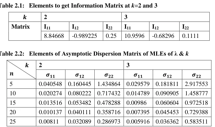
As the integrals involved in these mathematical expectations are not analytically tractable
we have evaluated them using 11- point Gauss-Laguerre quadrature formula (Rao et al.,
1966) for selected values of k in a standard density (λ=1) and are given in Table - 2.1.
The elements of the corresponding asymptotic dispersion matrix for selected values of k
are given in Table – 2.2.
Table 2.1: Elements to get Information Matrix at k=2and 3
2 3
Matrix I11 I12 I22 I11 I12 I22
8.84668 -0.989225 0.25 10.9596 -0.68296 0.1111
Table 2.2: Elements of Asymptotic Dispersion Matrix of MLEs of λ & k
2 3
5 0.040548 0.160445 1.434864 0.029579 0.181811 2.917553
10 0.020274 0.080222 0.717432 0.014789 0.090905 1.458777
When the log likelihood equations do not admit analytical expressions as MLEs of the parameters of a density function from complete or censored sample, replacement of certain portions of log likelihood equations by suitable admissible approximations sometimes would lead to simpler and efficient estimates of the parameters. Such estimates in literature are named as approximate or modified MLEs. Tiku (1967); Mehrotra and Nanda (1974); Pearson and Rootzen (1977); Tiku and Suresh (1992);
Rosaiah et al. (1993a); Rosaiah et al. (1993b); Kantam and Srinivasa Rao (1993);
Kantam and Srinivasa Rao (2002); Kantam and Sriram (2003); Kantam et al. (2013) and
the references therein are some of the works in this direction. We adopt this concept of MML estimation for Burr type X distribution by considering its reparameterised version as given in Raqab and Kundu (2006).
We see that the maximum likelihood estimator of the shape parameter k is a closed form
expression whereas, the maximum likelihood estimator of λ is an iterative solution of the
equation (2.2) involving k. In order to overcome the iterative nature of the solution we
proceed as follows. Equation (2.2) can be rewritten as
∑ ( ) ∑
(2.9)
.
Consider the expression ( )
(2.10)
of equation (2.9).
We approximate this expression by a linear one in in a small neighborhood of the
quantile of the population say
( ) . (2.11)
With this approximation, equation (2.9) becomes a quadratic equation in λ given by
(2.12)
where, ∑ ( ) ∑ ( ) ∑
Positive root of this equation is an estimate of λ called the modified maximum likelihood estimate (MMLE) of λ. It can be seen that A,B,C depend on the ordered observations
x1,x2,…,xn, the shape parameter k and the slope, intercept of the linear approximation
(2.11). In order to find , we suggest two methods.
Method-I:
Let
Let be the solutions of the following equations
( ) ( )
where √ √ F(.) is the cdf of standard Burr type X
The expressions for are
√ * ( √ ) +
(2.13)
√ * ( √ ) + (2.14)
The slope and intercept of the linear approximation in the equation (2.11) are given
by
( ) ( )
(2.15)
( ) (2.16)
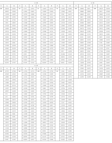
where βi is given by (2.15). The values of αi and βi in this method for n=5(5)25 for
k=0.25, 0.50, 1.50, 2, 2.5,3 are given in Table 2.3 in Appendix-I.
Method-II:
Considering Taylor‟s expansion of ( ) upto its first derivative w.r.t zi in a
neighborhood of population quantile corresponding to pi, we get
( ) (2.17)
( ) (2.18)
where is the quantile of Burr type X distribution, given as the solution of the equation
( )
i.e., √ * ( √ ) + (2.19)
It can be seen from (2.10) that
( ) ( )
( ) (2.20)
Substituting (2.19) in (2.20) we get
( ) ( )
( ) (2.21)
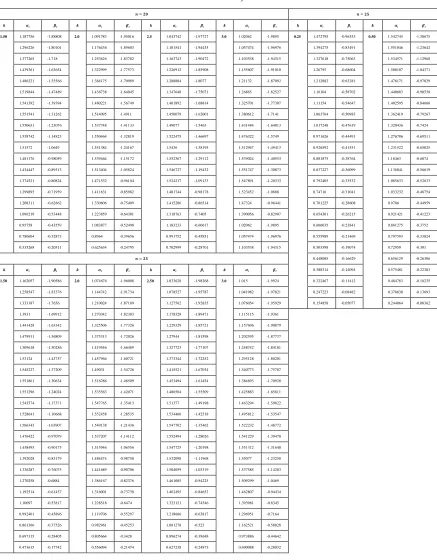
Using in (2.18) we get .
The values of and in this method for n=5(5)25 for k=0.25, 0.50, 1.5, 2, 2.5,3 are
depends on the size of the sample also. The larger the size, the narrower is the neighborhood and hence the closer is the approximation. That is, the exactness of the
approximation becomes finer and finer for large values of „n‟. Hence the approximate log
likelihood equation and the exact log likelihood equation tend to each other as n.
Hence the exact and modified MLEs are asymptotically identical (Tiku et al. 1986). The
same may not be true in small samples and these are to be assessed with the help of small
sample characteristics of the MMLEs. Because of non-tractability of analytical sampling
variances, we compared the modified ML method with exact ML method through Monte–Carlo simulation.
10,000 random samples of size n= 5 (5) 25 each are generated from Burr type X
distribution with k=0.25, 0.50, 1.5, 2, 2.5,3 in succession. For each sample at a given k
the and of Method-I (Method-II) as given in Table 2.3 (2.4) are used in equation
2.12 to get the modified MLE of „λ‟ by Method-I (Method-II). The empirical variances of MMLEs by Method-I and Method-II are respectively given in Table 2.5 in Appendix - III.
3. Estimation from Censored Samples
In life testing experiments censoring a given sample sometimes becomes necessary to save time and cost of experimentation. One common scheme of censoring is a failure
censored sample or a type II right censored sample, wherein pre-planned n items are put
to life testing and the experiment will be terminated as soon as a prefixed observations say „r‟ are noted down (r < n). In such situations, we are left with „r‟ actual observations say and the life times of the remaining (n-r) items are more than xr. Such a sample is called type – II right censored sample.
In this Section, we assume that we have a type – II right censored sample modeled by
Burr type X distribution with shape parameter „k‟ and scale parameter „λ‟. Maximum
likelihood estimation of scale parameter for a known shape parameter will be discussed below.
Let be a type – II right censored sample from a Burr type X
distribution in a planned random sample of sized „n‟. The likelihood function of such a
censored sample is given by α is
r n r
i r
i
k
x
F
k
x
f
(
;
,
).[
1
(
;
,
)]
1
(3.1)
where f(),F() respectively denote the probability density function and cumulative
distribution function of Burr type X distribution. Substituting the respective expressions
for f, F, taking natural logarithms, differentiating with respect to „λ‟ and on simplification
we get the estimating equation for the parameter „λ‟ as
∑ ( ) ∑
( )
( ) ( )( )
( )
(3.2)
It can be seen that for known value of k, the MLE of λ from censored sample is an iterative solution of equation (3.2). However, an analytical solution can be obtained by admissible modifications to some terms of equation (3.2) on lines of the procedures described in Section – 2. Consider the following two expressions of equation (3.2).
( )
(3.3)
( ) ( )( )
( ) (3.4)
We suggest to approximate ( ) of (4.3), ( ) of (3.4) by the following linear
expressions in small neighborhoods of population quantile, population quantile
respectively.
i.e., ( ) (3.5)
( ) (3.6)
Substituting these approximations in equation (3.2) and on simplification we get the following quadratic equation in „λ‟.
(3.7)
where ∑ (3.8)
( ) ∑ ( ) (3.9)
( ) ∑ ( ) (3.10)
Positive root of the above quadratic equation in (3.7) is taken as an estimate of λ called MMLE of λ from censored samples. We attempt to support our linear approximations for
( ) in the following way.
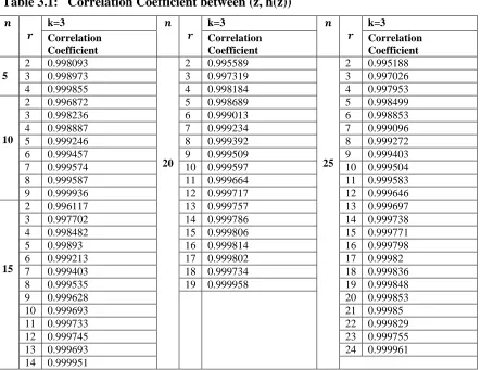
Let
√ √
be the solution of ( )
The interval ( ) is evenly divided by 10 cut off points say =z1<z2<…<z10= .
The Karl-Pearson‟s product moment correlation coefficient between ( ( )), i=1, 2,
3… 10 is calculated for n=5(5) 25 with all possible values of „r‟. These are given in Table
– 3.1 in Appendix - III, which show that there is a high linear relation between z and h(z)
indicating an acceptable linear approximation for h(z) in the neighborhood as
expressed in the equation
( ) . (3.11)
It can be seen that the constants A,B,C of the above quadratic equation in (3.7) depend on the values of the uncensored observations, size of the planned sample, number of
available observations, the known shape parameter k, the slopes and intercepts of the
linear approximations for ( ) of (3.5) and ( ) of (3.6). We suggest as in Section – 2,
two methods of finding these slopes and intercepts. It may also be noted that the slope
( ), the intercept ( ) in the linear approximation for ( ) remain unaltered from those
of Section - 2. The slope ( ) and the intercept ( ) of the linear approximation of ( )
will now be evaluated by methods – I and II of Section – 2.
Method – I:
Let .
√ √
Let be the respective solutions of ( ) ( ) ,
where F(.) is the CDF of Burr type X distribution.
i.e., √ ( ( ) ⁄ ) (3.12)
√ ( ( ) ⁄ ) (3.13)
The slope (
) ( )
(3.14)
and intercept ( ) (3.15)
The values of , for n=5(5)25, for all possible values of r within each „n‟ are
Method – II:
Expanding ( ) in Taylor series up to the first derivative in the neighborhood of the
quantile of the population and after some simplification we get
( ) (3.16)
From equation (3.4) we get that
( )
( ) *( ( ) ){( ) ( ) ( )} , ( ) -+
[ ( ) ]
(3.17)
Replacing z with in equation (3.17) we get
( )
( ) *( ( ) ){( ) ( ) ( )} , ( ) -+
* ( ) +
(3.18)
Let ( ) .
Then √ [ (
) ⁄
] (3.19)
( ) (3.20)
The values of , for n=5(5)25 and all possible values of r are given in Tables 3.8 to
3.13 in Appendix-V. From Bhattacharyya (1985) it follows that the MMLEs from censored samples are also asymptotically as efficient as MLEs.
In small samples the performance of MMLEs between the two methods of modification
is studied through Monte-Carlo simulation for selected values of n, r (to the extent of
20% censoring in each chosen value of n). That is, the selected combinations are
n=5,r=4; n=10,r=8; n=15,r=12; n=20,r=16; n=25,r=20. These are given in Table 3.14
Appendix - I
Table 2.3: Slope ( ) and Intercept ( ) in Modification to MLE by Method –I for n=5, 10, 15, 20
0.25 1.001544 -0.06947 0.25 1.000137 -0.02066 2.0 1.173059 -0.57054 0.25 1.000031 -0.00977 1.50 1.098443 -0.43888 1.002237 -0.15653 1.000165 -0.04796 1.176377 -0.58546 1.000035 -0.02292 1.100832 -0.45901 1.020322 -0.30384 1.001491 -0.09438 1.220816 -0.63942 1.000313 -0.04533 1.143291 -0.53186 1.080881 -0.48925 1.005975 -0.15585 1.245337 -0.66498 1.001251 -0.07506 1.177126 -0.58202 1.150719 -0.54725 1.016637 -0.23229 1.252992 -0.67115 1.003479 -0.11212 1.204841 -0.61856
0.50 1.027824 -0.2493 1.037497 -0.32307 1.241769 -0.65958 1.007835 -0.1565 1.226972 -0.6449 1.033775 -0.33597 1.073303 -0.42602 1.205548 -0.62816 1.015373 -0.20811 1.24326 -0.66247 1.100058 -0.49402 1.127991 -0.53443 1.131001 -0.57027 1.027354 -0.26679 1.252849 -0.67167 1.185074 -0.61542 1.195104 -0.62423 0.984942 -0.46837 1.045219 -0.3321 1.254213 -0.67217 1.24172 -0.66128 1.241632 -0.66093 0.935784 -0.44881 1.070507 -0.40319 1.244874 -0.66286
1.50 1.182883 -0.58678 0.50 1.00827 -0.13626 2.5 1.206809 -0.61719 1.104591 -0.47831 1.220775 -0.64161 1.190747 -0.61196 1.009135 -0.18243 1.208629 -0.62588 1.147842 -0.55364 1.174896 -0.60461 1.239253 -0.65949 1.027432 -0.27312 1.242211 -0.6619 1.196673 -0.62001 1.093706 -0.54452 1.207388 -0.62266 1.054795 -0.36228 1.253638 -0.67203 1.229891 -0.6498 0.944811 -0.44406 1.182908 -0.61317 1.090811 -0.44839 1.24682 -0.66458 1.255411 -0.67339 0.901456 -0.42827
2.0 1.223006 -0.63852 1.134264 -0.52887 1.220169 -0.641 0.50 1.003907 -0.09372 2.0 1.145468 -0.52655 1.22516 -0.64773 1.181872 -0.5988 1.168027 -0.59939 1.004177 -0.12522 1.147764 -0.5405 1.24143 -0.65818 1.224414 -0.64754 1.077988 -0.53385 1.012541 -0.18772 1.189346 -0.59877 1.166494 -0.58988 1.230982 -0.64614 0.91947 -0.42895 1.02509 -0.24989 1.218043 -0.63439 1.122837 -0.56967 1.240338 -0.65936 0.866911 -0.4078 1.041799 -0.31145 1.238066 -0.65684
2.5 1.245223 -0.66349 1.50 1.125535 -0.49283 3.0 1.229802 -0.64553 1.062591 -0.37204 1.250599 -0.66957 1.24134 -0.66169 1.129668 -0.51631 1.229873 -0.64953 1.087301 -0.43115 1.255704 -0.674 1.229046 -0.64573 1.181483 -0.59155 1.251994 -0.67091 1.115588 -0.48807 1.252718 -0.67057 1.122945 -0.55821 1.218877 -0.63751 1.25151 -0.66926 1.14679 -0.54168 1.240259 -0.65901 1.066949 -0.5316 1.243112 -0.66304 1.232594 -0.65192 1.179624 -0.59023 1.216007 -0.63835
3.0 1.255781 -0.67419 1.251484 -0.66968 1.193878 -0.62009 1.211546 -0.63084 1.176159 -0.60677 1.246254 -0.66445 1.237361 -0.65494 1.130075 -0.57196 1.237222 -0.65824 1.114203 -0.56097 1.20989 -0.62921 1.186527 -0.61116 1.029602 -0.50217 1.244227 -0.66175 1.017789 -0.49469 1.080905 -0.52942 1.062996 -0.51793 0.864134 -0.39689 1.196747 -0.61404 0.857917 -0.39339 1.016665 -0.49883 1.020774 -0.50184 0.809966 -0.37503 1.187022 -0.61676 0.811801 -0.37616
Appendix – I (Continued)
Table 2.3 (Continued): Slope ( ) and Intercept ( ) in Modification to MLE by Method –I for n=20, 25
1.50 1.082349 -0.40267 2.0 1.12777 -0.49543 2.5 1.164819 -0.55714 3.0 1.193592 -0.59892 0.25 1.000004 -0.0037 0.50 1.001479 -0.05769 1.083927 -0.42055 1.129445 -0.50833 1.166204 -0.56626 1.194464 -0.60511 1.000005 -0.00876 1.00154 -0.07698 1.119918 -0.48957 1.167338 -0.56656 1.201462 -0.6132 1.22501 -0.64179 1.000043 -0.0174 1.004622 -0.11545 1.149383 -0.53876 1.194992 -0.60454 1.224602 -0.64114 1.242742 -0.66125 1.00017 -0.02888 1.009246 -0.15387 1.17465 -0.57661 1.216345 -0.63134 1.240467 -0.65881 1.252899 -0.67154 1.000474 -0.04321 1.015413 -0.19218 1.19651 -0.60651 1.232809 -0.65047 1.250798 -0.66949 1.257349 -0.67562 1.001066 -0.06037 1.023121 -0.23035 1.215238 -0.63015 1.244968 -0.66362 1.256342 -0.67476 1.256901 -0.67489 1.002089 -0.08039 1.032364 -0.26832 1.230836 -0.64844 1.253007 -0.67169 1.257376 -0.67543 1.251869 -0.67007 1.003715 -0.10324 1.043131 -0.30601 1.243116 -0.66184 1.256848 -0.67515 1.253888 -0.67191 1.242269 -0.66151 1.006144 -0.12893 1.055404 -0.34335 1.251708 -0.67052 1.256201 -0.67417 1.245636 -0.66437 1.22789 -0.64934 1.009603 -0.15743 1.069153 -0.38025 1.256041 -0.67442 1.250557 -0.6687 1.232164 -0.65275 1.208307 -0.63349 1.01435 -0.18872 1.08433 -0.41658 1.255289 -0.67322 1.239151 -0.6585 1.21276 -0.63681 1.182859 -0.61375 1.020671 -0.22276 1.100865 -0.45218 1.248272 -0.6664 1.220875 -0.64308 1.186396 -0.61614 1.150583 -0.58972 1.028875 -0.25948 1.11865 -0.48687 1.233288 -0.65306 1.194131 -0.62168 1.151585 -0.59006 1.110092 -0.56078 1.039297 -0.29877 1.137526 -0.52038 1.207801 -0.63184 1.156561 -0.59313 1.106143 -0.55752 1.05936 -0.52601 1.052286 -0.34049 1.157255 -0.5524 1.167858 -0.60063 1.104525 -0.5556 1.046727 -0.51693 0.9953 -0.48398 1.068191 -0.3844 1.177482 -0.58246 1.106833 -0.55591 1.03201 -0.50613 0.96786 -0.4657 0.912886 -0.43238 1.087336 -0.43013 1.197669 -0.60997 1.012267 -0.49121 0.927889 -0.43927 0.859507 -0.39914 0.802972 -0.36708 1.109964 -0.47713 1.216991 -0.63407 0.854987 -0.39175 0.766522 -0.34273 0.698763 -0.30665 0.644812 -0.27875 1.136123 -0.5245 1.234142 -0.65355 0.812791 -0.37677 0.723591 -0.32722 0.656338 -0.29125 0.60336 -0.26369 1.165428 -0.57076 1.24699 -0.66655
1.19652 -0.61331 1.25187 -0.67014
1.225693 -0.64725 1.241994 -0.65932
1.50 1.071525 -0.37604 2.0 1.115236 -0.47176 2.50 1.152241 -0.53706 3.0 1.18188 -0.58232 1.242853 -0.66217 1.203239 -0.62441 1.072659 -0.39233 1.116526 -0.48382 1.153386 -0.54585 1.182687 -0.58855 1.215516 -0.63019 1.098987 -0.54209 1.104095 -0.45789 1.151321 -0.54107 1.187112 -0.59352 1.213117 -0.62714 1.216785 -0.63998 1.073867 -0.53682 1.130135 -0.50536 1.177333 -0.5795 1.210229 -0.62331 1.232173 -0.64938
Appendix – II
Table 2.4: Slope ( ) and Intercept ( ) in Modification to MLE by Method –II for n=5, 10, 15, 20
0.25 1.249164 -0.66728 0.25 1.369003 -0.80108 2.0 1.169044 -1.90112 0.25 1.421925 -0.87535 1.50 1.225577 -1.86011 1.032638 -0.48712 1.227534 -0.64647 1.310984 -1.7873 1.312165 -0.73308 1.349387 -1.74887 0.837227 -0.36099 1.107134 -0.543 1.423283 -1.65974 1.219567 -0.639 1.435953 -1.64161 0.638381 -0.25422 0.99642 -0.46171 1.502926 -1.51928 1.136041 -0.56619 1.495812 -1.53547 0.408803 -0.14952 0.889993 -0.39261 1.546091 -1.3664 1.057889 -0.50548 1.533399 -1.42939
0.50 1.497945 -1.01809 0.784217 -0.33074 1.547629 -1.20121 0.982965 -0.45254 1.550882 -1.32281 1.33462 -0.75879 0.675774 -0.27299 1.50011 -1.02333 0.9098 -0.4049 1.54924 -1.21534 1.136041 -0.56619 0.560626 -0.21685 1.391787 -0.83146 0.837227 -0.36099 1.528641 -1.10668 0.901726 -0.39986 0.432266 -0.15948 1.201172 -0.62214 0.764192 -0.31967 1.488557 -0.99648 0.603306 -0.2371 0.275998 -0.09586 0.876108 -0.38413 0.6896 -0.28007 1.427703 -0.88435
1.50 1.410392 -1.67716 0.50 1.546728 -1.19433 2.5 1.096036 -1.94764 0.612156 -0.24138 1.343793 -0.7697 1.541392 -1.39394 1.48529 -0.98934 1.215465 -1.86781 0.530129 -0.20276 1.232961 -0.65162 1.528641 -1.10668 1.399023 -0.84158 1.331993 -1.76681 0.440875 -0.16318 1.088414 -0.52846 1.374521 -0.80824 1.300797 -0.72057 1.433348 -1.64543 0.339641 -0.12101 0.896671 -0.39672 1.030754 -0.48577 1.19328 -0.61506 1.509276 -1.50373 0.215309 -0.07281 0.622995 -0.24665
2.0 1.289313 -1.80725 1.07626 -0.5192 1.549232 -1.34139 0.50 1.552458 -1.28535 2.0 1.119018 -1.93369 1.480221 -1.56749 0.947751 -0.42915 1.540639 -1.1576 1.528641 -1.10668 1.225577 -1.86011 1.552458 -1.28535 0.803547 -0.3416 1.46619 -0.95071 1.480384 -0.97894 1.318899 -1.77972 1.471532 -0.96104 0.63494 -0.25252 1.29738 -0.71686 1.421925 -0.87535 1.398141 -1.69287 1.158678 -0.58502 0.419563 -0.15407 0.970534 -0.44418 1.357266 -0.7862 1.462347 -1.59984
2.5 1.195363 -1.88263 1.50 1.287698 -1.80869 3.0 1.053683 -1.97185 1.287851 -0.70668 1.510406 -1.50084 1.401892 -1.68814 1.429281 -1.65129 1.145805 -1.91664 1.214131 -0.63397 1.540989 -1.396 1.534466 -1.42518 1.51191 -1.49693 1.252964 -1.83836 1.136041 -0.56619 1.552458 -1.28535 1.524217 -1.09133 1.549142 -1.34224 1.36101 -1.73634 1.053129 -0.50198 1.542733 -1.16885 1.25667 -0.6747 1.545511 -1.18584 1.456822 -1.6091 0.964558 -0.4402 1.509074 -1.04629
3.0 1.12898 -1.92745 1.50148 -1.02671 1.526279 -1.45485 0.868973 -0.37982 1.447701 -0.91727 1.325701 -1.77307 1.414249 -0.86371 1.552454 -1.27142 0.764192 -0.31967 1.353059 -0.78099 1.495812 -1.53547 1.276719 -0.69504 1.51257 -1.05589 0.646485 -0.25824 1.216186 -0.63586 1.547891 -1.20333 1.073224 -0.51691 1.370622 -0.80317 0.508628 -0.193 1.020295 -0.47834 1.332899 -0.75677 0.761866 -0.3184 1.050424 -0.49999 0.332728 -0.11823 0.723621 -0.29783
Appendix – II (Continued)
Table 2.4 (Continued): Slope ( ) and Intercept ( ) in Modification to MLE by Method –II for n=20, 25
1.50 1.187756 -1.88808 2.0 1.091783 -1.95016 2.5 1.043742 -1.97727 3.0 1.02062 -1.9895 0.25 1.472795 -0.96353 0.50 1.542745 -1.38675 1.296226 -1.80101 1.176436 -1.89603 1.101541 -1.94435 1.057474 -1.96976 1.394275 -0.83491 1.551046 -1.23642 1.377265 -1.718 1.253626 -1.83782 1.163743 -1.90472 1.103538 -1.94315 1.327618 -0.75063 1.534571 -1.12968 1.439361 -1.63654 1.322999 -1.77573 1.226912 -1.85908 1.155607 -1.91018 1.26795 -0.68604 1.508107 -1.04371 1.486221 -1.55566 1.384175 -1.70989 1.288804 -1.8077 1.21132 -1.87092 1.212882 -0.63281 1.476171 -0.97029 1.519844 -1.47489 1.436738 -1.64045 1.347648 -1.75071 1.26865 -1.82527 1.16104 -0.58702 1.440683 -0.90538 1.541392 -1.39394 1.480221 -1.56749 1.401892 -1.68814 1.325701 -1.77307 1.11154 -0.54647 1.402595 -0.84666 1.551541 -1.31262 1.514095 -1.4911 1.450079 -1.62001 1.380612 -1.7141 1.063764 -0.50983 1.362419 -0.79267 1.550631 -1.23076 1.537748 -1.41133 1.49077 -1.5463 1.431484 -1.64813 1.017248 -0.47619 1.320436 -0.7424 1.538742 -1.14823 1.550464 -1.32819 1.522475 -1.46697 1.476322 -1.5749 0.971626 -0.44491 1.276786 -0.69511 1.51572 -1.0649 1.551384 -1.24167 1.5436 -1.38195 1.512967 -1.49413 0.926592 -0.41551 1.231522 -0.65025 1.481176 -0.98059 1.539464 -1.15172 1.552367 -1.29112 1.539024 -1.40553 0.881875 -0.38764 1.18463 -0.6074 1.434447 -0.89513 1.513404 -1.05824 1.546727 -1.19432 1.551747 -1.30873 0.837227 -0.36099 1.136041 -0.56619 1.374521 -0.80824 1.471532 -0.96104 1.524217 -1.09133 1.547891 -1.20333 0.792405 -0.33532 1.085633 -0.52633 1.299895 -0.71959 1.411631 -0.85982 1.481744 -0.98178 1.523452 -1.0888 0.74716 -0.31041 1.033232 -0.48754 1.208311 -0.62862 1.330606 -0.75409 1.415206 -0.86514 1.47324 -0.96441 0.701225 -0.28608 0.9786 -0.44959 1.096219 -0.53448 1.223859 -0.64301 1.318763 -0.7405 1.390056 -0.82907 0.654301 -0.26215 0.921421 -0.41223 0.95758 -0.43559 1.083877 -0.52498 1.183233 -0.60617 1.02062 -1.9895 0.606035 -0.23841 0.861275 -0.3752 0.780604 -0.32873 0.8964 -0.39656 0.991752 -0.45851 1.057474 -1.96976 0.555989 -0.21469 0.797593 -0.33824 0.535268 -0.20511 0.625634 -0.24795 0.702999 -0.28701 1.103538 -1.94315 0.503598 -0.19074 0.72959 -0.301
0.448085 -0.16629 0.656129 -0.26306
0.388314 -0.14094 0.575481 -0.22383
1.50 1.162057 -1.90586 2.0 1.074676 -1.96008 2.50 1.033628 -1.98268 3.0 1.015 -1.9924 0.322467 -0.11412 0.484783 -0.18235
1.258547 -1.83376 1.144742 -1.91734 1.078527 -1.95787 1.041982 -1.97821 0.247223 -0.08482 0.378638 -0.13693 1.333187 -1.7656 1.210024 -1.87189 1.127562 -1.92835 1.076054 -1.95929 0.154858 -0.05077 0.244064 -0.08362 1.3931 -1.69912 1.270342 -1.82383 1.178328 -1.89471 1.115115 -1.9361
Appendix-III
Table 2.5: Empirical Variances of ̂ based on MMLE: Method –I & Method –II
MMLE: Method –I
0.25 0.50 1.50 2.0 2.5 3.0
5 0.1341425 0.097691 0.044699 0.035495 0.02685 0.02321 10 0.099113 0.060441 0.020486 0.016022 0.012314 0.010444 15 0.07457 0.038852 0.013336 0.010474 0.00819 0.006875 20 0.059105 0.028732 0.009685 0.00823 0.005912 0.005017 25 0.0469 0.021249 0.007989 0.006167 0.004862 0.004187 MMLE: Method –II
0.25 0.50 1.50 2.0 2.5 3.0
5 0.130502 0.099553 0.040283 0.028477 0.019177 0.013697 10 0.097346 0.057394 0.018313 0.012291 0.008974 0.00647 15 0.079233 0.038871 0.011892 0.007887 0.005866 0.004383 20 0.064955 0.028415 0.008615 0.006064 0.00426 0.003162 25 0.053599 0.020655 0.006947 0.00485 0.003434 0.0025
Table 3.1: Correlation Coefficient between (z, h(z))
k=3 k=3 k=3
Correlation Coefficient
Correlation Coefficient
Correlation Coefficient
5
2 0.998093
20
2 0.995589
25
2 0.995188
3 0.998973 3 0.997319 3 0.997026
4 0.999855 4 0.998184 4 0.997953
10
2 0.996872 5 0.998689 5 0.998499
3 0.998236 6 0.999013 6 0.998853
4 0.998887 7 0.999234 7 0.999096
5 0.999246 8 0.999392 8 0.999272
6 0.999457 9 0.999509 9 0.999403
7 0.999574 10 0.999597 10 0.999504
8 0.999587 11 0.999664 11 0.999583
9 0.999936 12 0.999717 12 0.999646
15
2 0.996117 13 0.999757 13 0.999697
3 0.997702 14 0.999786 14 0.999738
4 0.998482 15 0.999806 15 0.999771
5 0.99893 16 0.999814 16 0.999798
6 0.999213 17 0.999802 17 0.99982
7 0.999403 18 0.999734 18 0.999836
8 0.999535 19 0.999958 19 0.999848
9 0.999628 20 0.999853
10 0.999693 21 0.99985
11 0.999733 22 0.999829
12 0.999745 23 0.999755
13 0.999693 24 0.999961
Appendix - IV
Table 3.2: Slope ( ) and Intercept ( ) in Modification to MLE from Censored Sample by Method –I: k=0.25
0.25
5 2 3.473945 0.087458 0.25 25 2 7.652104 0.019929 3 3.758664 0.093293 3 5.561148 0.03954 4 4.879543 -0.2058 4 4.560551 0.058519 10
2 4.171105 0.048719 5 4.000841 0.076474 3 3.504577 0.090939 6 3.665968 0.092919 4 3.354078 0.117855 7 3.463801 0.107262 5 3.463016 0.114755 8 3.348766 0.118779 6 3.769879 0.055961 9 3.296087 0.126585 7 4.289639 -0.10754 10 3.291509 0.129589 8 5.115904 -0.48441 11 3.326662 0.126444 9 6.551342 -1.39176 12 3.396789 0.115459 15 2 5.265932 0.032981 13 3.499593 0.094491 3 4.07629 0.064297 14 3.634655 0.060776 4 3.574889 0.092048 15 3.803218 0.010684 5 3.365154 0.113558 16 4.008237 -0.06067 6 3.318288 0.125085 17 4.254695 -0.16001 7 3.383293 0.121334 18 4.550294 -0.29696 8 3.540161 0.094621 19 4.906744 -0.48575 9 3.785417 0.033383 20 5.342221 -0.7486 10 4.128378 -0.08071 21 5.886358 -1.12252 11 4.593546 -0.27881 22 6.591664 -1.67524 12 5.231281 -0.6192 23 7.565199 -2.54986 13 6.150807 -1.22836 24 9.095302 -4.1429 14 7.655368 -2.466
20
Table 3.3: Slope ( ) and Intercept ( ) in Modification to MLE from Censored Sample by Method –I: k=0.50
0.50
5 2 1.826788 -0.08609 0.50 25 2 1.159598 -0.00321 3 2.415824 -0.31404 3 1.243444 -0.00985 4 3.289925 -0.8439 4 1.330307 -0.02019 10
2 1.400954 -0.02038 5 1.420469 -0.03454 3 1.631698 -0.06555 6 1.514261 -0.05325 4 1.890025 -0.14219 7 1.612065 -0.07677 5 2.185062 -0.26078 8 1.714327 -0.10559 6 2.531458 -0.43886 9 1.821572 -0.14035 7 2.954923 -0.70845 10 1.934425 -0.18178 8 3.507629 -1.13701 11 2.053629 -0.23079 9 4.330148 -1.91053 12 2.180088 -0.28852 15 2 1.266246 -0.00896 13 2.314904 -0.35637 3 1.411523 -0.02804 14 2.45945 -0.43611 4 1.566639 -0.05873 15 2.61546 -0.53007 5 1.733364 -0.10301 16 2.785168 -0.64126 6 1.914005 -0.16355 17 2.971528 -0.77378 7 2.111638 -0.244 18 3.178554 -0.93333 8 2.330478 -0.34953 19 3.411915 -1.12813 9 2.576509 -0.48772 20 3.680009 -1.37068 10 2.858645 -0.67022 21 3.996102 -1.68119 11 3.191033 -0.91612 22 4.383204 -2.0956 12 3.598311 -1.25975 23 4.887602 -2.68785 13 4.130188 -1.7724 24 5.633568 -3.659 14 4.920114 -2.64884
Table 3.4: Slope ( ) and Intercept ( ) in Modification to MLE from Censored Sample by Method –I: k=1.50
1.50
5 2 1.037595 -0.43145 1.50 25 2 0.418654 -0.09955 3 1.390186 -0.74688 3 0.554401 -0.16364 4 1.752863 -1.143 4 0.666795 -0.22453 10
2 0.705847 -0.22912 5 0.765727 -0.28406 3 0.929575 -0.37878 6 0.855712 -0.34306 4 1.120058 -0.52797 7 0.939347 -0.40208 5 1.29607 -0.68457 8 1.018326 -0.46155 6 1.468208 -0.85582 9 1.093854 -0.52187 7 1.646176 -1.05229 10 1.16685 -0.58341 8 1.84409 -1.29439 11 1.238062 -0.64656 9 2.096124 -1.63751 12 1.308135 -0.71176 15 2 0.561846 -0.15872 13 1.377662 -0.77948 3 0.740641 -0.26088 14 1.447222 -0.85033 4 0.889665 -0.35945 15 1.51742 -0.925 5 1.022675 -0.45807 16 1.588929 -1.00441 6 1.146155 -0.55883 17 1.662549 -1.08973 7 1.264116 -0.66359 18 1.739287 -1.1826 8 1.37957 -0.77438 19 1.820503 -1.28532 9 1.495225 -0.89375 20 1.90816 -1.40135 10 1.614016 -1.02532 21 2.005341 -1.53631 11 1.739774 -1.17472 22 2.117433 -1.70024 12 1.1878524 -1.35181 23 2.255529 -1.9141 13 2.042019 -1.57693 24 2.450671 -2.23697 14 2.262397 -1.90695
Table 3.5: Slope ( ) and Intercept ( ) in Modification to MLE from Censored Sample by Method –I: k=2.0
2.0
5 2 0.91197 -0.48689 2.0 25 2 0.370266 -0.12903
3 1.197436 -0.77718 3 0.495 -0.20352
4 1.467311 -1.10273 4 0.596585 -0.2713 10
2 0.628161 -0.27758 5 0.684557 -0.33524 3 0.824474 -0.43362 6 0.763285 -0.39663 4 0.984712 -0.57881 7 0.835287 -0.4563 5 1.126877 -0.72222 8 0.902198 -0.51483 6 1.260369 -0.87035 9 0.965167 -0.57269 7 1.392817 -1.03116 10 1.025057 -0.63029 8 1.534198 -1.21889 11 1.082551 -0.688 9 1.707694 -1.47203 12 1.138216 -0.74622 15 2 0.499965 -0.19869 13 1.192555 -0.80532 3 0.661061 -0.31108 14 1.246035 -0.86576 4 0.79155 -0.41369 15 1.29912 -0.92805 5 0.904879 -0.51165 16 1.352304 -0.99283 6 1.007294 -0.60758 17 1.406152 -1.06092 7 1.102542 -0.7034 18 1.461356 -1.13342 8 1.193281 -0.80092 19 1.518835 -1.21189 9 1.281731 -0.90213 20 1.579904 -1.2987 10 1.370112 -1.00963 21 1.646627 -1.39769 11 1.46113 -1.12732 22 1.722641 -1.5158 12 1.558884 -1.26195 23 1.81552 -1.66773 13 1.671285 -1.42752 24 1.946813 -1.89572 14 1.820208 -1.66392
Table 3.6: Slope ( ) and Intercept ( ) in Modification to MLE from Censored Sample by Method –I: k=2.5
2.5
5 2 0.823503 -0.51529 2.5 25 2 0.340376 -0.14995 3 1.062195 -0.77978 3 0.455794 -0.23008 4 1.272799 -1.05175 4 0.548491 -0.30086 10
2 0.57515 -0.30804 5 0.627713 -0.36598 3 0.750018 -0.46366 6 0.697703 -0.42714 4 0.888111 -0.60149 7 0.760902 -0.48537 5 1.006713 -0.73168 8 0.81889 -0.5414 6 1.114436 -0.86044 9 0.872771 -0.59576 7 1.217708 -0.9943 10 0.923362 -0.64891 8 1.324215 -1.14403 11 0.971302 -0.70123 9 1.451093 -1.33836 12 1.017109 -0.75307 15 2 0.459334 -0.22543 13 1.061229 -0.8048
3 0.605895 -0.34181 14 1.104064 -0.85677 4 0.721962 -0.44405 15 1.145999 -0.90941 5 0.82062 -0.53845 16 1.187427 -0.96319 6 0.907894 -0.62807 17 1.228784 -1.01873 7 0.987327 -0.71498 18 1.270591 -1.07684 8 1.06135 -0.80089 19 1.313524 -1.13868 9 1.131893 -0.8875 20 1.358547 -1.20596 10 1.20077 -0.97686 21 1.407172 -1.28153 11 1.27007 -1.07189 22 1.462075 -1.37057 12 1.342836 -1.17758 23 1.528889 -1.4842 13 1.42488 -1.3043 24 1.623858 -1.65491 14 1.53241 -1.48217
Table 3.7: Slope ( ) and Intercept ( ) in Modification to MLE from Censored Sample by Method –I: k=3.0
3.0
5 2 0.756006 -0.52925 3.0 25 2 0.318752 -0.16504 3 0.960339 -0.77042 3 0.426364 -0.24819 4 1.130073 -1.00107 4 0.511761 -0.31999 10
2 0.534895 -0.32762 5 0.583937 -0.3848 3 0.69274 -0.48003 6 0.647017 -0.44465 4 0.813998 -0.6099 7 0.703372 -0.50073 5 0.915303 -0.72823 8 0.75453 -0.55387 6 1.00469 -0.84113 9 0.801555 -0.60468 7 1.087804 -0.95427 10 0.845229 -0.65364 8 1.170898 -1.07623 11 0.886153 -0.70113 9 1.267362 -1.22952 12 0.924814 -0.74752 15 2 0.428985 -0.24373 13 0.961616 -0.79313 3 0.563638 -0.36103 14 0.996919 -0.83829 4 0.668287 -0.46109 15 1.031056 -0.88335 5 0.755655 -0.55109 16 1.064358 -0.92869 6 0.831562 -0.63447 17 1.09718 -0.97481 7 0.899384 -0.71341 18 1.129937 -1.02234 8 0.96139 -0.78958 19 1.163158 -1.07216 9 1.019314 -0.86453 20 1.197591 -1.1256 10 1.074712 -0.93995 21 1.234406 -1.18488 11 1.129285 -1.01818 22 1.275687 -1.25405 12 1.185431 -1.10308 23 1.325857 -1.34195 13 1.247665 -1.20273 24 1.397816 -1.47476 14 1.328662 -1.34098
Appendix - V
Table 3.8: Slope ( ) and Intercept ( ) in Modification to MLE from Censored Sample by Method –II: k=0.25
0.25
5 2 3.267468 0.132721
0.25 25
2 7.627645 0.038197 3 3.44044 0.094053 3 5.534529 0.056735 4 4.241724 -0.20182 4 4.531775 0.074491 10
2 4.095068 0.08669 5 3.96987 0.091067
3 3.414306 0.119652 6 3.632716 0.105979 4 3.245847 0.135306 7 3.428117 0.118636 5 3.329058 0.119951 8 3.310425 0.128328 6 3.595149 0.05074 9 3.254772 0.134187 7 4.04402 -0.11357 10 3.246787 0.135158
8 4.73059 -0.457 11 3.277958 0.12994
9 5.811663 -1.18651 12 3.343353 0.116917 15 2 5.220663 0.061262 13 3.44044 0.094053 3 4.025095 0.089076 14 3.568497 0.058746 4 3.517373 0.11263 15 3.728354 0.007603 5 3.300446 0.129289 16 3.922384 -0.06389 6 3.244853 0.13544 17 4.154731 -0.16187 7 3.298651 0.12607 18 4.431818 -0.295 8 3.44044 0.094053 19 4.763314 -0.47585 9 3.664566 0.028894 20 5.163908 -0.72359 10 3.976672 -0.08561 21 5.656724 -1.06909 11 4.394443 -0.27606 22 6.2805 -1.56615 12 4.953784 -0.58979 23 7.106836 -2.3194 13 5.726488 -1.12145 24 8.291435 -3.57152 14 6.875098 -2.09775
Table 3.9: Slope ( ) and Intercept ( ) in Modification to MLE from Censored Sample by Method –II: k=0.50
0.50
5 2 1.775421 -0.13818
0.50 25
2 1.158527 -0.00616 3 2.292353 -0.36648 3 1.241604 -0.01418 4 2.988413 -0.82167 4 1.327531 -0.02581 10
2 1.391967 -0.03671 5 1.41658 -0.04135 3 1.614299 -0.0881 6 1.509064 -0.06115 4 1.860575 -0.16884 7 1.605344 -0.08563 5 2.138313 -0.28809 8 1.705841 -0.11527 6 2.459047 -0.46074 9 1.811046 -0.15066 7 2.841793 -0.71263 10 1.921537 -0.19251 8 3.321357 -1.09387 11 2.038004 -0.24168 9 3.973092 -1.72028 12 2.161274 -0.29924 15 2 1.262809 -0.01674 13 2.292353 -0.36648 3 1.405268 -0.03918 14 2.432481 -0.44507 4 1.556705 -0.07278 15 2.583211 -0.53714 5 1.718723 -0.11937 16 2.746521 -0.64544 6 1.893383 -0.1814 17 2.92499 -0.77367 7 2.083383 -0.26222 18 3.122069 -0.9269 8 2.292353 -0.36648 19 3.342526 -1.1123 9 2.52533 -0.50088 20 3.593223 -1.34053 10 2.7896 -0.67546 21 3.884577 -1.62822 11 3.09627 -0.90616 22 4.233591 -2.00349 12 3.463551 -1.22021 23 4.671077 -2.51926 13 3.924596 -1.66958 24 5.263125 -3.29443 14 4.550783 -2.37251
2 1.197748 -0.00955 3 1.302675 -0.0221 4 1.412264 -0.04052 5 1.527098 -0.06544 6 1.647871 -0.09767
20
Table 3.10: Slope ( ) and Intercept ( ) in Modification to MLE from Censored Sample by Method –II: k=1.50
1.50
5 2 1.075006 -0.51634
1.50 25
2 0.460274 -0.13029 3 1.374915 -0.78692 3 0.583236 -0.18976 4 1.675123 -1.1163 4 0.688548 -0.24778 10
2 0.757851 -0.2895 5 0.782621 -0.30509 3 0.956607 -0.4247 6 0.868898 -0.36218 4 1.131581 -0.56311 7 0.949507 -0.41947 5 1.294999 -0.7093 8 1.025894 -0.47731 6 1.454811 -0.86867 9 1.099116 -0.53604 7 1.618304 -1.04925 10 1.169994 -0.59599 8 1.795003 -1.2653 11 1.239203 -0.65751 9 2.002707 -1.54842 12 1.30733 -0.72101 15 2 0.610889 -0.20436 13 1.374915 -0.78692 3 0.771343 -0.29794 14 1.442485 -0.85578 4 0.909809 -0.39078 15 1.510586 -0.92824 5 1.035201 -0.4846 16 1.579818 -1.0051 6 1.152455 -0.58086 17 1.650884 -1.08742 7 1.264848 -0.68107 18 1.72465 -1.17661 8 1.374915 -0.78692 19 1.802254 -1.27464 9 1.484949 -0.9006 20 1.885286 -1.3844 10 1.597383 -1.02512 21 1.976123 -1.51037 11 1.715246 -1.16503 22 2.078649 -1.66011 12 1.842967 -1.32783 23 2.199996 -1.84789 13 1.988195 -1.52758 24 2.355862 -2.10621 14 2.167279 -1.79612
20
Table 3.11: Slope ( ) and Intercept ( ) in Modification to MLE from Censored Sample by Method –II: k=2.0
2.0
5 2 0.950885 -0.56721
2.0 25
2 0.411493 -0.164 3 1.191522 -0.81173 3 0.523443 -0.23198 4 1.416142 -1.08187 4 0.617976 -0.29579 10
2 0.679382 -0.34035 5 0.701163 -0.35674 3 0.851468 -0.47838 6 0.776299 -0.41568 4 0.997524 -0.61126 7 0.84543 -0.4732 5 1.129003 -0.74399 8 0.90994 -0.5298 6 1.252859 -0.88122 9 0.97083 -0.58586 7 1.374824 -1.02886 10 1.028866 -0.64174 8 1.501658 -1.1967 11 1.084659 -0.69778 9 1.645321 -1.40606 12 1.138726 -0.75433 15 2 0.548399 -0.24827 13 1.191522 -0.81173 3 0.691257 -0.34925 14 1.243472 -0.87039 4 0.811518 -0.44458 15 1.294995 -0.93077 5 0.917732 -0.53683 16 1.346532 -0.99345 6 1.014589 -0.62777 17 1.398581 -1.05915 7 1.105111 -0.71891 18 1.451735 -1.12881 8 1.191522 -0.81173 19 1.506763 -1.20378 9 1.275696 -0.90789 20 1.564722 -1.28598 10 1.359475 -1.00956 21 1.627195 -1.37846 11 1.445006 -1.11985 22 1.696778 -1.48637 12 1.535293 -1.24382 23 1.778282 -1.61956 13 1.635435 -1.39096 24 1.882446 -1.80076 14 1.75637 -1.58302
20
Table 3.12: Slope ( ) and Intercept ( ) in Modification to MLE from Censored Sample by Method –II: k=2.5
2.5
5 2 0.861412 -0.59062
2.5 25
2 0.380247 -0.18713 3 1.061074 -0.81049 3 0.483127 -0.25948 4 1.236938 -1.03581 4 0.568948 -0.32557 10
2 0.624105 -0.37079 5 0.643548 -0.38724 3 0.775859 -0.5065 6 0.710111 -0.44563 4 0.90096 -0.63146 7 0.77061 -0.50152 5 1.010278 -0.75121 8 0.826378 -0.55548 6 1.110135 -0.87009 9 0.878372 -0.60798 7 1.205369 -0.99288 10 0.927315 -0.6594 8 1.301218 -1.1269 11 0.973778 -0.71008 9 1.406477 -1.28769 12 1.018229 -0.76034 15 2 0.505884 -0.2765 13 1.061074 -0.81049 3 0.634713 -0.37973 14 1.102677 -0.86088 4 0.741024 -0.47385 15 1.143386 -0.91187 5 0.833067 -0.56212 16 1.183553 -0.96389 6 0.915332 -0.64663 17 1.223562 -1.01748 7 0.99066 -0.72896 18 1.26386 -1.07334 8 1.061074 -0.81049 19 1.305013 -1.13244 9 1.128203 -0.89265 20 1.347792 -1.19618 10 1.193554 -0.97711 21 1.393349 -1.2668 11 1.25879 -1.0662 22 1.443579 -1.34808 12 1.326139 -1.16362 23 1.502026 -1.44738 13 1.399321 -1.27627 24 1.576698 -1.58188 14 1.486334 -1.42021
20
Table 3.13: Slope ( ) and Intercept ( ) in Modification to MLE from Censored Sample by Method –II: k=3.0
3.0
5 2 0.792232 -0.59996
3.0 25
2 0.357065 -0.20337 3 0.961963 -0.7983 3 0.452459 -0.27784 4 1.103985 -0.98907 4 0.531195 -0.34448 10
2 0.581344 -0.38937 5 0.59893 -0.40557 3 0.717204 -0.52084 6 0.658748 -0.46247 4 0.826482 -0.63772 7 0.712562 -0.5161 5 0.91957 -0.74603 8 0.761658 -0.56713 6 1.002343 -0.84997 9 0.806955 -0.61606 7 1.079056 -0.95366 10 0.849143 -0.66331 8 1.153999 -1.06288 11 0.888761 -0.70923 9 1.234031 -1.18959 12 0.926244 -0.75413 15 2 0.473417 -0.29512 13 0.961963 -0.7983
3 0.590945 -0.39819 14 0.996242 -0.84204 4 0.686315 -0.48965 15 1.029382 -0.88566 5 0.767512 -0.57335 16 1.061682 -0.9295 6 0.838856 -0.65164 17 1.093453 -0.974 7 0.903046 -0.72617 18 1.125052 -1.01969 8 0.961963 -0.7983 19 1.156921 -1.06732 9 1.017069 -0.86929 20 1.189658 -1.11796 10 1.069661 -0.94055 21 1.224149 -1.17333 11 1.121098 -1.01389 22 1.261861 -1.23637 12 1.173135 -1.09218 23 1.035553 -1.31285 13 1.228647 -1.18071 24 1.361532 -1.41644 14 1.293826 -1.29196
2 0.405112 -0.24001 3 0.510002 -0.32609 4 0.595903 -0.40277 5 0.669416 -0.47292 6 0.734121 -0.53826
20
Appendix- VI
Table 3.14: Empirical Variances of MMLE of λ from Censored Sample: Method –
I & Method –II
MMLE: Method –I
( )
0.25 0.50 1.50 2.0 2.5 3.0
(5,4) 11.49365 0.412213 0.18131 0.187485 0.21507 0.245198
(10,8) 0.410329 0.11826 0.103083 0.125636 0.150761 0.182708
(15,12) 0.138162 0.075133 0.040271 0.109317 0.131422 0.16653
(20,16) 0.092643 0.055522 0.071039 0.091347 0.12222 0.150345
(25,20) 0.067846 0.042435 0.067635 0.089057 0.114548 0.150973
MMLE: Method –II
( )
0.25 0.50 1.50 2.0 2.5 3.0
(5,4) 5.027481 0.388384 0.179044 0.193406 0.21721 0.737996
(10,8) 0.534766 0.103742 0.100408 0.120603 0.151993 0.180261
(15,12) 0.180459 0.065647 0.082163 0.102875 0.130453 0.162365
(20,16) 0.109447 0.047965 0.072703 0.092277 0.122778 0.149991
(25,20) 0.083155 0.038627 0.066796 0.084847 0.113837 0.146095
References
1. Bhattacharyya, G.K. (1985). The Asymptotic of Maximum Likelihood and
Related Estimators based on Type II Censored Data. Journal of American
Statistical Association, Vol.80, 398-404.
2. Burr, I.W. (1942). Cumulative Frequency Functions. The Annals of Mathematical
Statistics, Vol.13, 215-232.
3. Gupta, R.D., and Kundu D. (1999). Generalized Exponential Distributions.
Australian and New Zealand Journal of Statistics, Vol.41, No.2, 173-188.
4. Kantam, R.R.L., Priya, M.Ch. and Ravikumar, M.S. (2013). Modified Maximum
Likelihood Estimation in Linear Failure Rate Distribution. Inter Stat, July.
5. Katnam, R.R.L. and Ravikumar, M.S. (2015). Modified Maximum Likelihood
Estimation in Burr Type X Distribution. Inter Stat, June, 1-14.
6. Kantam, R.R.L., and Srinivasa Rao, G. (1993). Reliability Estimation in Rayleigh
Distribution with Censoring – Some Approximations to ML Method. Proceedings
7. Kantam, R.R.L., and Srinivasa Rao, G. (2002). Log-logistic Distribution:
Modified Maximum Likelihood Estimation. Gujarat Statistical Review, Vol. 29,
No. 1 & 2, 25-36.
8. Kantam, R.R.L., and Sriram, B. (2003). Maximum Likelihood Estimation from
Censored Samples – Some Modifications in Length Biased Version of
Exponential Model. Statistical Methods, Vol. 5, No. 1, 63-78.
9. Kundu, D., and Raqab, M. Z. (2005). Generalized Rayleigh Distribution:
Different Methods of Estimation. Computational Statistics & Data Analysis,
Vol. 49, 187-200.
10. Mehrotra, K.G., and Nanda, P. (1974): Unbiased Estimation of Parameters by
Order Statistics in the case of Censored Samples, Biometrika, Vol. 61, 601-606.
11. Mudholkar, Govind S., and Srivastava, Deo Kumar. (1993). Exponentiated
Weibull family for analyzing bathtub failure-rate. Reliability, IEEE Transaction,
Vol.42, No.2, 299 - 302.
12. Pearson, E.S., and Rootzen, H. (1977). Simple and Highly Efficient Estimators for
a Type-I Censored Normal Sample. Biometrika, Vol. 64, No. 1, 123-128.
13. Rao, C.R., Mathai, A., and Mitra, S.K. (1966). Formulae and Tables for Statistical
Work. Statistical Publishing Society, Calcutta, India.
14. Raqab, M. Z., and Kundu, D. (2006). Burr type X distribution: revisited. Journal
of Probability and Statistical Science, Vol.8, 179-198.
15. Rosaiah, K., Kantam, R.R.L., and Narasimham, V.L. (1993a). ML and Modified
ML Estimation in Gamma Distribution with a Known Prior Relation Among the
Parameters. Pakistan Journal of Statistics, Vol. 9, No. 3(B), 37-48.
16. Rosaiah, K., Kantam, R.R.L., and Narasimham, V.L. (1993b). On Modified
Maximum Likelihood Estimation of Gamma Parameters. Journal of Statistical
Research, Bangladesh, Vol. 27, No. 1&2, 15-28.
17. Tiku, M.L (1967). Estimating the Mean and Standard Deviation from a Censored
Normal Sample. Biometrika, Vol. 54, 155-165.
18. Tiku, M.L., and Suresh, R.P. (1992). A New Method of Estimation for Location
and Scale Parameters. Journal of Statistical Planning & Inference, Vol. 30, 281-292.
19. Tiku, M.L., Tan, W.Y., and Balakrishnan, N. (1986). Robust Inference. Marcel