under Model Selection Uncertainty
Georges Nguefack-Tsague
University of Yaounde I Biostatistics Unit
Abstract
Model selection uncertainty would occur if we selected a model based on one data set and subsequently applied it for statistical inferences, because the “correct” model would not be selected with certainty. When the selection and inference are based on the same dataset, some additional problems arise due to the correlation of the two stages (selection and inference). In this paper model selection uncertainty is considered and model averaging is proposed. The proposal is related to the theory of James and Stein of estimating more than three parameters from independent normal observations. We suggest that a model averaging scheme taking into account the selection procedure could be more appropriate than model selection alone. Some properties of this model averaging estimator are investigated; in particular we show using Stein's results that it is a minimax estimator and can outperform Stein-type estimators.
Keywords: James and Stein estimator, Model selection, Model averaging, Minimax, Normal multivariate mean.
1. Introduction
Stein (1956) considered the problem of estimating several parameters from independent normal observations, and showed that it was possible to uniformly improve on the maximum likelihood estimator under the total squared error risk measure in dimension three and higher. The setting relating to Stein's estimation is as follows: Let
1
= (X , ,Xp)
X have a p-dimensional multivariate normal distribution
2
( , ),
p p
N I
X (1)
with unknown mean = ( ,1 ,p),
known (for simplicity) and Ip the identity covariance matrix; thus X can be observed from p independent experiments. An estimator ˆ = ( ,ˆ1 ,ˆp) of
is evaluated by the risk function2
ˆ
( , ) = ,
R E
where 2 2
=1
ˆ = p (ˆi i)
i
and E stands for averaging over the sample space with respect to the distribution (1).Under (1), the maximum likelihood estimator (MLE) is
ˆML = .
X
This MLE was long though to be the “best” estimator for the multivariate mean estimation problem; i.e. it was believed that no estimator existed that achieved a lower risk. Pursuing the work of Stein (1956), James and Stein (1961) showed that if p3 the following estimator of the multivariate mean
2 2
( 2) ˆ = (1JS p )
X
X
achieves uniformly lower risk than the MLE for all parameter values
; i.e.ˆ ˆ
( , ) < ( , ) .
JS JS ML ML
R R
The statistical community was astonished by the proof of James and Stein estimator (JSE) in 1961 (Efron and Morris 1977). Many statisticians were skeptical about JSE (mainly) because it does not share many of the nice properties of the MLE; e.g. it is nonlinear, biased and with probability density function (pdf) which cannot be expressed in a closed form (Efron and Morris 1977, Richards 1998). JSE is now well known and accepted among statisticians and econometricians (Judge and Bock 1978, Greenberg and Webster 1998, Lehman and Casella 1998, Gruber 1998). Several other drawbacks of JSE have been pointed out and many efforts have been made to improve. One major drawback is that the region of the parameter space where the risk of JSE (or some other estimators of a similar type) is significantly smaller than that of the MLE is quite limited (see Akai 1989, Stein 1981, Berger 1982).
Stein (1966) discussed Stein-type estimators for designs admitting a completely orthogonal analysis of variance. He showed that for large sample size, the Stein-type estimator applied separately to each orthogonal subspace is approximatively better than the estimator which shrinks observations towards the general average. Haff (1978) considered the estimator of normal means which are close to each other. He obtained a minimax estimator which is a modification of a Stein-type estimator shrinking observations towards the grand average. Efron and Morris (1973) considered the estimation of normal means divided in two groups with different prior variances and proposed a compromise estimator which improved the risk of Stein-type estimator. Berger and Dey (1983) did the same for k groups, leading also to an improvement of Stein-type estimator. George (1986a,b,c,d) considered situations where only conflicting or vague prior information is available; and proposed minimax estimators called multiple shrinkage Stein estimators. Akai (1989) proposed improvement over MLE when observations are classified into several groups. Since the discovery of JSE, many others shrinkage techniques have evolved. References include Efron and Morris (1975), Fay and Herriot (1979), Rubin (1981), Morris (1983), Jones (1991), Brown (2008), and Brown et al. (2011).
the models under consideration. This leads to the class of model averaging estimators. Several options are available for specifying the weights; e.g. they can be based on the Akaike's information criterion, AIC (Akaike 1973) or Bayesian information criterion, BIC (Schwarz 1978). It is not the construction of the estimator that causes difficulties; the problem is to determine its properties. The same problem arises for estimators obtained after model selection. We refer to these estimators as post-model selection estimators (PMSE, Leeb and Pötscher 2005). The inferences are invalid even if different datasets are used for selection and inference because the uncertainty (variation) in the selection is ignored.
Let M = {M1, ,MK} be a set of K plausible models to estimate ˆ , the quantity of interest. Denote by ˆk the estimator of k obtained when using model Mk. Model
averaging involves finding non-negative weights, w1, ,wK, that sum to one, and then estimating
by=1
ˆ = ˆ . K
k k k
w
(2)
Clearly, model selection is a special case of model averaging, with one of the weights set to unity, and all the others to zero, i.e the estimator based on a selection procedure is a mixture (0-1 weight) of the candidate estimators ˆ1, ,ˆK.
Literature on PMSEs includes, inter alia, Bancroft (1944) for pretest estimators, Breiman (1992), Hjorth (1994), Chatfield (1995), Draper (1995), Buckland et al. (1997), Zucchini (2000), Candolo et al. (2003), Hjort and Claeskens (2003), Efron (2004), Leeb and Pötscher (2005), Longford (2005), Claeskens and Hjort (2008), Zucchini et al. (2011), Nguefack-Tsague and Zucchini (2011), Nguefack-Tsague et al. (2011), Nguefack-Tsague (2013a,b,c), and Zhang et al. (2014).
Some model averaging weights base the weights on penalized likelihood values. Some classical weights can be seen in Buckland et al. (1997), Hjort and Claeskens (2003). Hansen (2007, 2008, 2009, 2010) and Wan et al. (2010) derived optimal weighting scheme by minimizing a Mallows'Cp criterion (Mallows 1973). Nguefack-Tsague (2014) derived optimal weights with squared error loss and showed that they may exist in theory but once estimated they are no longer optimal. Bayesian model averaging can be found in Hoeting (1999) and Wasserman (2000). Numerous applications of Akaike weights are given in Burnham and Anderson (2002).
The model selection criterion determines which model is assigned the weight one and
hence used to estimate
. The index of the selected model, k, is a random variable. We denote the selected model byk
M , and the PMSE of the quantity of interest by ˆ
k
. Let ()
I denote the indicator function that has the value 1 if the argument is true, and 0 if it is false. Then
=1 =1
ˆ ˆ
= ( ) , = ( ) .
K K
k k
k k
k k
Clearly, the properties of ˆ
k
depend on (among other things) the set of candidate models, , and on the selection procedure, which we denote by S.
Nguefack-Tsague and Zucchini (2011) proposed a model averaging estimator in which the selection procedure is taken into account. Their proposal depends on estimators
( k| ) = Pr( k | ), = 1,
p M S M is selected S k K and the maximized likelihood value Lk for
each model Mk. These weights are given by
=1
( | )
( ) = , = 1, 2, , ;
( | )
k k
k K
i i
i
p M S L
W S k K
p M S L
(3)with its associated model averaging estimator given by
=1
ˆ( ) = ( )ˆ . K
k k
k S W S
(4)Nguefack-Tsague and Zucchini (2011) showed that this weighting scheme dominates classical model averaging estimators and PMSEs in a simple linear regression example. The problem that needs to be solved is that of constructing estimators, p M S( k| ), of the model selection probabilities. Hjort and Claeskens (2003) showed that a naive bootstrap estimator of the selection probability of model Mk (namely the proportion of resamples
in which Mk is selected) does not work. If the selection probabilities depend on some
parameter for which a closed form expression exists, and if one can find an estimator of the parameter, then it is possible to obtain estimators for these probabilities. For the case where there is no closed form, Miller (2002) suggested using a Monte Carlo method based on projection.
We consider the estimation of a multivariate mean when many estimators are plausible for a set of K models. Instead of selecting one of them using a specific selection criterion, we average over all these estimators by taking account this selection criterion (see Nguefack-Tsague and Zucchini 2011). Although each of the competing estimators does not necessary follow a multivariate normal distribution, it is assumed that the true model (i.e. the one that generated the data) does. It is also assumed that the model selection probabilities are computed independently from the data, for example using the Monte Carlo procedure of Miller (2002).
An example of estimators for each model Mk could be those proposed by George (1986a, page 189):
2
2 ˆ =k ( k)[min(1, )]
k p
X X
X (5)
where kRp is fixed, thus X shrinks towards a target k for each model Mk. In particular if for each model Mk, k =0, then ˆ0 is the original positive part of Stein
This paper considers Stein's estimation problem where many models are a-priori plausible. In this situation one often uses the data to select the ``best" model; this model is then used to make inferences, ignoring model selection uncertainty, i.e. the fact that the selection step and inference were carried out using the same data. We suggest that a model averaging scheme taking into account the selection procedure could be more appropriate than model selection alone. For example, instead of selecting one estimator over those given in Equation (5), we propose to average over K estimators in which the selection procedure is taken into account in the weighting scheme. In particular, this example shows that it is possible to average over Stein-type estimators (which already outperform MLE ) and obtain a better estimator. Some properties of this model averaging estimator are investigated; in particular we showed using Stein's results that it is a minimax estimator and can outperformed Stein-type estimators. A Bayesian approach for estimating a multivariate mean under model uncertainty is considered in Nguefack-Tsague (2013c).
This paper is organized as follows. In Section 2 we define some concepts and the properties of the model averaging estimator. We show in Section 3 that it can improve over Stein-type estimators while Section 4 deals with a construction of confidence interval using this estimator. Our article ends with concluding remarks.
2. Definitions and properties of the model averaging estimator
2.1 Definitions
Definition 1. An estimator
is minimax if( , ) ( , ) ;
supR supR for any other estimator
i.e. the largest risk of
is no greater than that of any other estimator (the best worst-case scenario).Definition 2. An estimator
is said to dominate estimator
if*
( , ) ( , ) .
R R for alland if there exists some value for which the inequality is strict
Definition 3. An estimator
is said to admissible if there is no other estimator that dominates it (otherwise it is inadmissible).Definition 4. A function : Rh p R is said to be almost differentiable if there exists a function h: Rp R such that, for all z,
1 0
( ) ( ) = ( )
h x z h x
z h x tz dt for almost all xRp; where is the vector differential operator of first partial
derivatives with ith coordinate i = i x
. A function : R R
p p
g is almost
Definition 5. A lower semicontinous function f : Rp R { } is superharmonic at point x0Rp if for every r> 0, the average of f over the sphere
2 2
0 0
( ) = { : } =
r
S x x xx r
of radius r centered at x0 is not greater than f x( 0).
Definition 6. A twice continuously differentiable function f : Rp R is harmonic at x0
Rp
if 2f x( ) = 0;0 where 2 2
=1
= p i
i
is the Laplacian.2.2 Properties of the model averaging estimator
Let H: Rp R be defined by H(X| ,S M)=
=1 ( | )
K
k k
k p M S L
(denominator of themodel averaging weight defined in Equation (3). In addition, suppose that for each model
k
M , the estimator ˆk is of the form X logLk;MkM , where
1
log log
log = ( k, , k)
k
p
L L
L
x x
. The estimator of the form "X logLk" is motivated
by Stein (1981) who explains that small risk may be obtained by such estimator (see also George (1986a, page 190)). We write down in the following the risk of the proposed model averaging estimator given in Equation (4) and prove that it is a minimax estimator for
.Assumptions
A.1. X Np( , 2Ip),
known.A.2. H is almost differentiable for which H is also almost differentiable. A.3. H is superharmonic.
A.4.
2 2
( | , ) /
| |< ,
( | , )
i
H S M X
E
H S M
X
X for = 1,i ,p.
A.5. E logH(X| ,S M) 2<.
Lemma 1.The model averaging estimator in Equation (4) becomes
ˆ( ) =S logH( | ,S M).
Proof. Denote 1 = ( , , ) p f f f x x
and =
f Logf f . =1 =1 =1 =1 =1 =1 ( | ) ˆ( ) = ( )ˆ = { }ˆ ( | , ) 1
= ( | ) [ log ]
( | , ) 1 = ( | ) [ ] ( | , ) 1 = ( | ) ( | , ) 1 = ( ( | ) ) ( | , ) 1
= ( | , ) = log (
( | , )
K K k k
k k k
k k
K
k k k
k K k k k k k K k k k K k k k
p M S L
S W S
H S M
p M S L X L
H S M
L p M S L
H S M L
p M S L
H S M
p M S L
H S M
H S M H
H S M
X X X X X X X XX X X
X X| ,S M)
Lemma 2 (Lemma 1 of Stein (1981, page 1136)). Let Y be a N(0,1) real random variable and let g: RR be an indefinite integral of the Lebesgue measurable function
g, essentially the derivative of g. If E g Y| ( ) |<, then { ( )} = {E g Y E Yg Y( )}.
Lemma 3 (Lemma 2 of Stein (1981, page 1137)). If h: Rp R is an almost differentiable function with E h( ) <X , then Eh( ) =X E{(X) ( )}h X .
Lemma 4 (Theorem 4.8 of Helms (1969, page 63)). If f : Rp R is twice continuous differentiable, then f is superharmonic in Rp if and only if, for all
Rp
X ,
2
( ) 0
f
X .
Lemma 5 (Theorem 1 of Stein (1981, page 1138)). Consider an estimator Xg( )X for
such that g: Rp Rp is an almost differentiable function for which=1
{ p | i i( ) |} < 0
i
E
g X , then for each i{1, , }p ,2 2
{ i i( ) i} = 1 { i( ) 2 i i( )},
E X g X E g X g X and consequently
2 2
( ) = { ( ) 2 . ( )}.
E Xg X pE g X g X
(7)
Theorem 1. Under the assumptions A.1-A.5, ˆ ( ) S has risk
2
2 ( | , )
ˆ ˆ
( ( ), ) = ( ) = 4 [ ]
( | , ) H S M
R S E S p E
H S M
X
X
Proof. Let g: Rp Rp be defined by
= log = H.
g H
H
(8)
Then
2 2
2
. = . logg H = H H ,
H H
it follows from Equation (7) that
Note that 2 ( | , ) = . ( | , ) = . ( | , )
2 ( | , )
H S M
H S M H S M
H S M
X X X
X
2
( | , ) ( | , )
= .
2 ( | , ) 4[ ( | , )] ( | , )
H S M H S M
H S M H S M H S M
2
X X
X X X (9)
Thus
2 2
2
2 ( | , ) ( | , )
4 ( | , ) =
( | , ) [ ( | , )] ( | , )
2 ( | , ) ( | , ) ( | , ) ( | , )
=
( | , ) ( | , )
H S M H S M
H S M
H S M H S M H S M
H S M H S M H S M H S M
H S M H S M
2 2 2 X X X
X X X
X X X X
X X
.
It follows that
2 2
4 ( | , ) 2 ( | , ) ( | , )
=
( | , ) ( | , )
( | , )
H S M H S M H S M
H S M H S M
H S M
2 2
X X X
X X X . Thus 2 ( | , ) ˆ
( ( ), ) = 4 [ ]
( | , ) H S M
R S p E
H S M
X
X .
From Equation (9),
2
2 ( | , )
( | , ) 0
2 ( | , ) H S M H S M
H S M
X X
X since H is superharmonic
and by Lemma 4, 2H(X| ,S M) 0.
Since X is minimax for
with risk p,it then follows that R( ( ), )ˆ S p=infgsupE Xg( )X
3. Improvement over James-Stein estimator
Efron and Morris (1971, 1972) propose the following modification of the James-Stein estimator
2 2
( 2) ˆJSM = (1 p )
X
X
where a =aI a( 0).
distribution of ˆ|i| is skewed. We now also consider a modification of Efron and Morris based on order statistic.
Let Yi =|Xi | and the order statistics defined by Y(1) < <Y( )p . Let j p be a positive integer. Suppose also that the coordinates of (g X| ,S M) in Equation (8) as g=logH
are now defined as
2 2 1
( ) (j)
=1
2 2 1
( ) =1
[ (min( , ))] if
( | , ) =
[ (min( , ))] sign otherwise
p
l j i i
l
i p
l j i i
l
c X Y X Y Y
g S M
c X Y X X
X (10)where c is a constant. Let ( )S the corresponding model averaging estimator from Equation (6) with g defined as in Equation (10).
Theorem 2. The risk of ( ) S is given by
2 2 2 2 1
( ) =1
( ( ), ) = ( ) = ( 2( 2) ) [ (min( , ))] ]. p
l j l
R S E S p c j c E
X Y (11)Proof: Using equation (7) of Lemma 5,
2 2 2 1 2 2 1
( ) ( )
=1 =1 =1
1 2 2 2 2 2 2 2 2
( ) ( ) ( )
=1 =1 =1
2 2 2 1
( ) =1
( ( ), ) = [ [ (min( , ))] ] 2 ([ (min( , ))] )
4 [ (min( , ))] 4 ( 1) [ (min( , ))] ]
= ( 2( 2) ) [ (min( , ))]
p j p
l j l j
l i l
j p p
i l j j l j
i l l
p
l j l
R S p E c X Y c X Y
c X X Y c p j Y X Y
p c j c E X Y
]Corollary 1. The optimum choice of c is c* = j2 with its associated risk given by
2 2 2 2 1
( ) =1
( ( ), ) = ( ) = ( 2) [ (min( , ))] ]. p
l j l
R S E S p j E
X Y (12)Proof: Taking the derivative of the risk in Equation (11) with respect to c and equating to 0 yields c* = j2; replacing c by j2 in Equation (11) yields the risk in Equation (12)
Assume that p is large (p ) and z= j
p , so that j is close to p; and that i( )S are
independently normally distributed with variance 2. The estimated improvement risk for ( ) S and ˆJSM over the MLE ˆML are denoted respectively by Imp( ( ), S ˆML) and
ˆ ˆ
( JSM, ML)
Imp :
2 2 2 1
( ) =1
2 2 1
=1
ˆ ˆ
ˆ ˆ ˆ ˆ
( ( ), ) = ( , ) ( ( ), ) = ( 2) [ (min( , ))] ( , )
ˆ ˆ ˆ ˆ
= ( , ) ( , ) = ( 2) [ ] .
p
ML ML JSM ML
l j l p ML JSM l l
Imp S R R S j X Y Imp
R R p X
The asymptotic relative efficiency (Stein, 1981; page 1146) of ( )S compared to the modified James-Stein estimate ˆJSM is defined by
2 2
ˆ ˆ
( , )
( ) = = ,
ˆ
( ( ), ) (1 ) 2 ( )
JSM ML
ML
Imp z
eff z
Imp S z w w w z
(13)
where w=1(0.5(1z)), with and respectively as density and distribution functions of standard normal.
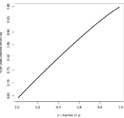
Figure (1) shows that the relative efficiency is an increasing function of z, i.e. as the proportion of data increases, the relative efficiency also increases. It also shows that in Equation(13), eff ( ) < 1,z z (0,1); thus ˆR( ( ), ) < ( S Rˆ ˆJSM, ) .
Asymptotic relative efficiency of ( )S compared to the modified James-Stein estimate ˆJSM
as a function of the proportion of the dimension of the parameter
.This means that the modified version of the weighted estimator (model averaging) given in Equation (10) is better than Jame-Stein estimator, for any proportion z of the data. When z= 1, that is p= j, eff(1)=1, then both estimators have the same improvement over the maximum likelihood estimator.
4. Confidence sets for the mean
Here we illustrate how to obtain an approximate confidence sets for the parameter
.Lemma 6. (Theorem 3 of Stein (1981, page 1149)). Let X be a random p-dimensional coordinate vector, normally distributed with mean
and the identity as covariancematrix. Let g: Rp Rp be a twice continuously differentiable function such that
2 2 2
{ ( ) ij( ) iij( )} < ,
where gij =jgi and giij = i jgi. Then
2 2
[ ( ) ( )] = ( )
E Xg X U X V X (15)
where
2
( ) = ( ) 2 ( )
U X p g X g X and
2 2
( ) = 2 4 [ ( ) 2 ( ) { ( )} ]
V X p E g X g X tr g X ,
and g denotes the vector-value function whose value is the transpose of the value of the function g.
Theorem 3. Let (g X| ,S M) =logH(X| ,S M). Under ((14)) with p ,
2
ˆ
[ ( ) ( | , )] = 2 4 [ ( | , )],
E S U X S M p E U X S M (16)
where U(X| ,S M) = p g(X| ,S M) 2 2 g(X| ,S M) and
2 2
( | , ) = 2 4 [ ( | , ) 2 ( | , ) { ( | , )} ]
V X S M p E g X S M g X S M tr g X S M
Proof. This is a straightforward application of Lemma 6 with
( | , ) = log ( | , )
g X S M H X S M .
As noted by Stein (1981, page 1150),
2 2 2
ˆ
[ ( ) { ( | , ) 2 ( | , )}]
E S p g X S M g X S M is approximately normally
distributed with mean 0 and that
2 2
2p4E[ g(X| ,S M) 2 g(X| ,S M) tr{ g(X| ,S M)} ] is approximately constant.
Thus a confidence sets for
with approximately 1 of covering
can be given by2
1
ˆ
= { : ( ) < ( | , ) ( | , )}
CS S U X S M Z W X S M ,
where
2 2
( | , ) = 2 4[ ( | , ) 2 ( | , ) { ( | , )} ]
W X S M p g X S M g X S M tr g X S M
5. Concluding Remarks
6. Acknowledgments
We thank the Editor-in-Chief and three anonymous reviewers whose constructive comments and suggestions have led to an improvement on earlier versions of this paper.
References
1. Akai, T. (1989). Simultaneous estimation of means of classified normal observations. Annals of the Institute of Statistical Mathematics, 41, 485–502. 2. Akaike, H. (1973). Information theory and an extension of the maximum
likelihood principle. In Second International Symposium on Information Theory, eds. B. Petrovand F. Csa´ki, Budapest: Akade´miai Kiado´, 267–281. 3. Bancroft, T.A. (1944). On bias in estimation due to the use of preliminary tests of
significance. Annals of Mathematical Statistics, 15, 190–204.
4. Berger, J. (1982). Selecting a minimax estimator of a multivariate normal mean.
Annals of Statistics, 10, 81–92.
5. Berger, J. and Dey D. (1983). Combining coordinates in simultaneous estimation of normal means. Journal of Statistical Planning and Inference, 8, 143–160. 6. Breiman, L. (1992). The little boot strap and other methods for dimensionality
selection in regression: X-Fixed predictor error. Journal of the American Statistical Association, 87, 738–754.
7. Brown, L.D. (2008). In-season prediction of batting averages: a field test of empirical Bayes and Bayes methodologies. Annals of Applied Statistics, 2, 113–152.
8. Brown, L. D., Nie, H. and Xie, X. (2011). Ensemble minimax estimation for multivariate normal mean. Submitted to Annals of Statistics.
9. Buckland, S.T., Burnham, K.P. and Augustin, N.H. (1997). Model selection: An integral part of inference. Biometrics, 53, 603–618.
10. Burnham, P.K. and Anderson, D.R. (2002). Model Selection and Multi model Inference, a practical Information-Theoretic Approach. 2nd Edition. Springer-Verlag: New York.
11. Candolo, C., Davison, A.C. and Deme´trio, C.G.B. (2003). A note on model uncertainty in linear regression. The Statistician, 158, 165–177.
12. Chatfied, C. (1995). Model Uncertainty, data mining and statistical inference (with discussion). Journal of the Royal Statistical Society, series B, 158, 419–466.
13. Claeskens, G. and Hjort, N.L. (2003). The focused information criterion. Journal of the American Statistical Association, 98, 900–916.
14. Claeskens, G. and Hjort, N.L. (2008). Model selection and model averaging, Cambridge University Press, Cambridge.
15. Draper, D. (1995). Assessment and propagation of model uncertainty (with discussion). Journal of the Royal Statistical Society, series B 57, 45–97.
17. Efron, B. and Morris, C. (1971). Limiting the risk of Bayes and empirical Bayes estimators- Part I: The Bayes case. Journal of the American Statistical Association, 66, 807–815.
18. Efron, B. and Morris, C. (1972). Limiting the risk of Bayes and empirical Bayes estimators- Part I: The empirical Bayes case. Journal of the American Statistical Association, 67, 130–139.
19. Efron, B. and Morris, C. (1973). Combining possibly related estimation problem.
Journal of the Royal Statistical Society, series B 35, 379–421.
20. Efron, B. and Morris, C. (1975). Data analysis using Stein’s estimator and its generalizations. Journal of the American Statistical Association, 70, 311–319. 21. Efron, B. and Morris, C. (1977). Stein’s paradox in statistics. Scientific
American, 236 (5), 119–127.
22. Fay, R. E. III and Herriot, R.A. (1979). Estimates of income for small places: an application of James-Stein procedures to census data. Journal of the American Statistical Association, 74, 269–277.
23. George, E.I. (1986a). Minimax multiple shrinkage estimation. Annals of Statistics, 14, 188–205.
24. George, E. I. (1986b). Combining minimax shrinkage estimators. Journal of the American Statistical Association, 81, 437–445.
25. George, E.I. (1986c). A formal Bayes multiple shrinkage estimator. Communications in Statistics. A-Theory and Methods, 15, 2099–2114.
26. George, E.I. (1986d). Multiple shrinkage generalizations of the James-Stein estimator. Contributions to the Theory and Applications of Statistics, Academic Press, New York.
27. Greenberg, E. and Webster, C.E. (1998). Advanced econometrics: a bridge to the literature, John Wiley and Sons, New York.
28. Gruber, M.H.J. (1998). Improving efficiency by shrinkage: the James-Stein and Ridge regression estimators, Marcel Dekker: New York.
29. Haff, L.R. (1978). The multivariate normal mean with intra class correlated components: estimation of urban fire alarm probabilities. Journal of the American Statistical Association, 60, 806–825.
30. Hansen, B.E. (2007). Least squares model averaging. Econometrica, 75, 1175–1189.
31. Hansen, B.E. (2008). Least squares forecast averaging. Journal of Econometrics, 146, 342–350.
32. Hansen, B.E. (2009). Averaging estimators for regressions with a possible structural break. Econometric Theory, 35, 1498–1514.
33. Hansen, B.E. (2010). Averaging estimators for auto regressions with an ear unit root. Journal of Econometrics, 158, 142–155.
34. Helms, L. (1969). Introduction to potential theory, John Wiley and Sons, New York.
35. Hjort, N.L. and Claeskens, G. (2003). Frequentist model average estimators.
36. Hjorth, J. (1994). Computer intensive statistical methods: Validation, model selection and bootstrap, Chapman and Hall, London.
37. Hoeting, J., Madigan D., Raftery A. and Volinsky C. (1999). Bayesian model averaging: A tutorial. Statistical Science, 4, 382–417.
38. Jones, K. (1991). Specifying and estimating multilevel models for geographical research. Transactions of the institute of British geographers, 16, 148–159. 39. James, W. and Stein, C. (1961). Estimation with quadratic loss. In Proceedings
for the Third Berkeley Symposium on Mathematical Statistics and Probability 1, 361–379. University of California Press.
40. Judge, G. and Bock, M. (1978). The statistical implications of pre-test and Stein rule estimators in Econometrics, North Holland, Amsterdam.
41. Leeb, H. and Potscher, B.M. (2005). Model selection and inference: Fact and fiction. Econometric Theory, 21, 21–59.
42. Lehmann E.L. and Casella G. (1998). Theory of point estimation. Springer (Second Edition), New York.
43. Linhart, H. and Zucchini, W. (1986). Model selection. John Wiley and Sons, New York.
44. Longford, N.T. (2005). Editorial: Model selection and efficiency-is’ which model...?’ The right question? J.R. Statist. Soc. A, 168, Part3, 469–472.
45. Mallows, C.L. (1973). Some comment son Cp. Technometrics, 15, 661–675. 46. Mc Quarrie, A.D.R. and Tsai, C.L. (1998). Regression and time series model
selection, World Scientific, Singapore.
47. Miller, A.J. (2002). Subset selection in regression, 2nd Edition, Chapman and Hall, London.
48. Morris, C. (1983). Parametric empirical Bayes inference: theory and applications. Journal of the American Statistical Association, 78, 47–55.
49. Nguefack-Tsague G. (2014). On optimal weighting scheme in model averaging.
American Journal of Applied Mathematics and Statistics, 2(3), 150–156.
50. Nguefack-Tsague G. (2013a). On boot strap and post-model selection inference.
International Journal of Mathematics and Computation, 21 (4), 51–64.
51. Nguefack-Tsague G. (2013b). An alternative derivation of some commons distributions functions: A post-model selection approach. International Journal of Applied Mathematics and Statistics, 42(12), 138–147.
52. Nguefack-Tsague, G. (2013c). Bayesian estimation of a multivariate mean under model uncertainty. International Journal of Mathematics and Statistics, 13, 83–92.
53. Nguefack-Tsague, G. and Zucchini, W. (2011). Post-model selection inference and model averaging. Pakistan Journal of Statistics and Operation Research, 7 (2-Sp), 347–361.
55. Richards, J. A. (1999). An Introduction to James-Stein Estimation, M.I.T. EECS Area Exam Report.
56. Rubin, D. (1981). Using empirical Bayes techniques in the law school validity studies. Journal of the American Statistical Association, 75, 801–827.
57. Schwarz, G. (1978). Estimating the dimension of a model. The Annals of Statistics, 6, 461–464.
58. Stein, C.M. (1956). Inadmissibility of the usual estimator for the mean of a multivariate distribution. In Proceedings for the Third Berkeley Symposium on Mathematical Statistics and Probability, 1, 197–206. University of California Press.
59. Stein, C.M. (1966). An approach to the recovery of inter-block information in balanced incomplete block designs. Festschrift (ed. F. N. David), 351-366, John Wiley and Sons, New York.
60. Stein, C.M. (1981). Estimation of the mean of a multivariate normal distribution. Annals of statistics. 9, 1135–1151.
61. Wan, A.T. K., Zhang X. and Zou G. (2010). Least squares model averaging by Mallows criterion. Journal of Econometrics, 156(2), 277–283.
62. Wasserman, L. (2000). Bayesian model selection and model averaging. Journal of Mathematical Psychology, 44, 92–107.
63. Zhang X., Zou G. and Liang H. (2014). Model averaging and weight choice in linear mixed-effects models. Biometrika, 101(1), 205–218.
64. Zucchini, W. (2000). An introduction to model selection. Journal of Mathematical Psychology, 4, 41–61.