Sanjay Kumar Prasad
Indian Agricultural Statistics Research Institute Library Avenue, PUSA, New Delhi
Lalmohan Bhar
Indian Agricultural Statistics Research Institute Library Avenue, PUSA, New Delhi
Abstract
Analysis of experimental data from Bayesian point of view has been considered. Appropriate methodology has been developed for application into designed experiments. Normal-Gamma distribution has been considered for a prior distribution. Developed methodology has been applied to real experimental data taken from long term fertilizer experiments.
Keywords: Bayesian analysis, Normal-gamma prior, Posterior distribution, Experimental design, Long term fertilizer experiments.
1. Introduction
Bayesian inference is an approach to statistics in which all forms of uncertainty are expressed in terms of probability. A Bayesian approach to a problem starts with the formulation of a model that is adequate to describe the situation of interest. As opposed to the point estimators used by classical statistics, Bayesian statistics is concerned with generating the posterior distribution of the unknown parameters given both the data and appropriate prior density for the parameters. As such, Bayesian statistics provides a much more complete picture of the uncertainty in the estimation of the unknown parameters, especially after the confounding effects of nuisance parameters are removed. Bayesian statistics has the advantage, in comparison to traditional statistics, of being easily established and derived. Intuitively, methods become apparent which in traditional statistics give the impression of arbitrary computational rules. For more details one may refer to Savage (1972), Raiffa and Schlaifer (1961), DeGroot (1970) and Berger (1985).
incorporating such information into the design process. By including prior data in the current analysis, the researcher avails himself of additional degrees of freedom that can reduce inference error risk in the current experiment and increase the precision with which results can be reported. That is to say, such a strategy has the potential to significantly reduce uncertainty, thereby improving the quality of the final result.
A Bayesian approach to design gives a mechanism for formally incorporating prior information into the design process. The subject design of experiments has two major components; first component deals with designing the experiment and the second component deals with analysis of the data generated from design of experiments. A lot of literature is available on designing the experiments from Bayesian point of view. Most of the research work centers around obtaining optimal designs. For an excellent review on Bayesian design of experiments one may refer to Chaloner and Verdinelli (1995). It seems that not much attention has been paid to the analysis component. Apart from Flournoy (1993), there are no “true case studies” that we know of where Bayesian ideas have been formally applied to the design of an actual scientific experiment before it is done. The Bayesian analysis of experimental data is considered by Broemeling (1985) and Box and Tiao (1973). The method of Box and Tiao (1973) uses numerical integration to isolate the marginal posterior distribution of each of the variance components, where as method of Broemeling (1985) is based on analytical approximation. Tsutakawa (1972) argued that when Bayesian inference is considered appropriate, it may be desirable to use two separate priors, one for constructing designs and the other for subsequent inference. Etzione and Kadane (1993) and Lindley and Singpurwalla (1991) considered the use of informative priors for design and noninformative priors for the subsequent statistical analysis. Wang and Hsu (2006) gave Bayesian analysis of the additive mixed model for Randomized Block Designs. This paper deals with the Bayesian analysis of the additive mixed model experiments.
In the present study an attempt has been taken to explore the use of Bayesian techniques for analyzing experimental data. Appropriate methodologies for analyzing experimental data from Bayesian point of view have been developed. Before considering the analysis of experimental data, the concept of Bayesian inference has been introduced. Bayesian concept is first explained then its extension to general linear model context is discussed. Then how this concept is used in designed experiments has been explained. Some examples are provided to explain the concept of Bayesian analytical technique for experimental data. In Section 2 concept of Bayesian inference has been introduced. Application of Bayesian inference to general linear model has also been discussed in this Section. Appropriate modification has been done for application into designed experiments. This is the subject matter of Section 3. In Section 4, application of the Bayesian methodologies is considered. Some real experimental data from long term fertilizer experiments have been taken for this purpose. The paper ended with a Section on Discussion.
2. Bayesian Inference
calculation of the posterior density of the parameters and sometimes calculation of the predictive distribution of future observations. The prior information is expressed by a probability density ( ), of the parameter of the model f( | ),x ,x s, where f is density of a random variable x, s is the sample space and is the parametric space. The
information in the data x= ( ,x x1 2,...,xn), where x1, x2, …, xn, is a random sample from a population with density f is contained in likelihood function L( | ) x , which is the joint density of the sample data. Then this is combined with the prior density of, by Bayes’ theorem, and gives the posterior density of. Thus one may describe inference problem in terms of (S, , ( ), f ( | ))x and this problem is solved once the posterior density
( | ) L( | ) ( )
x x (2.1)
is calculated.
From the posterior density one may make inference for by examining the posterior density. Some prefer to give estimates of either in point or interval estimates which are computed from the posterior distribution. If is one dimensional, a plot of its posterior density tells one the story about. But if is multidimensional one must be able to isolate those components of θ(now it is a vector of parameters) in which one is interested. Posterior inference mainly involves estimation, tests of hypothesis and prediction of future observation. In design of experiments, we are mainly interested in testing the significance difference between a pair of treatment effects. Thus our main concern here is tests of hypothesis. Regardless of what particular activity is contemplated, one must first find the posterior density of θ.Often all the components of θ are of interest, but sometimes some of these components θ1(say) are regarded as nuisance parameters and the remaining θ2 are of primary interest. How should one make inferences aboutθ2? The Bayesian will use
1
2( 2| ) ( ,1 2| )d 1 2 2 ( 1 2)
θ x θ θ x θ θ (2.2)
2
is called the marginal posterior density of θ2, and as with any posterior density function it may be used to estimate and test hypothesis concerning θ2.
2.1 Testing of Hypothesis
To test hypothesis about the parameterθ2, one perhaps would find a (1) Highest Posterior Density (HPD), 0 1, region R ( θ2) from 2(θ x2| ). Such a region has a property that if θ'2R ( θ2) and θ''2R ( θ2), then 2( ' | )θ2 x 2( '' | )θ 2 x , that is parameter values inside the region have larger posterior probability density than those excluded from the region which must satisfy
2 2
2 2 2
( )
1 ( | )
R
d
θ
θ x θ , (2.3)
that is the HPD region has posterior probability content 1. To test the hypothesis
0: 2 20
2.2 Bayesian Analysis in General Linear Model [Broemeling, 1985]
Let θ be a p1 vector of real parameters, Y(y y1, 2,...,yn)' a n1 vector of observations, X a np known design matrix. Then the general linear model is
Y Xθ e (2.4)
where e~N(0,1Ιn) and Ιn is the precision matrix of e, which has covariance matrix
2 ,
Ιn and 2 1 0 is unknown.
Here our objective is to provide inference for θ and after observings(y , y ,..., y1 2 n). In Bayesian analysis all inferences are based on the posterior distribution ofθ. Suppose one’s prior information about θ is represented by a probability density function
θ θ Rp
( , ), , 0,
then Bayes’ theorem combines this information with the information contained in the sample. The likelihood functions for θ and is
2
2
θ s n / Y Xθ Y Xθ
L( , | ) exp ' , (2.5)
The likelihood function is one’s sample information about the parameters and is the conditional density function of the sample random variables given θ and . Bayes’ theorem gives the conditional density of θ given s as
( , | )θ s L( , | ) ( , ),θ s θ
(2.6)
The posterior density of θ is ( , | )θ s and represents one’s knowledge of θ and after observing the sample s. On the other hand our information about θ and before s is observed is contained in the prior density.
From (2.6) the posterior density can be written as
( , | )θ s K.L( , | ) ( , ),θ s θ
(2.7)
where K is a normalizing constant and is given by
1
0
K
L( , | ) ( , )d d ,θ θ θ p
R
s (2.8)
which is the marginal probability density of Y.
2.2.1 Normal-Gamma Prior Density
The prior information about θ and can be given in many ways. In the present study we consider the case when ( , )θ is Normal-Gamma prior density, i.e., prior distribution of
θ is Normal and that of is Gamma, i.e.,
1 2
( , )θ ( | )θ ( ),
(2.9)
where
2 1
2
θ p / θ - μ)'P(θ - μ
( | ) exp ( )
μ is a p1 given vector and Ρ is known pp positive definite matrix. Thus 1 is conditional density of θ given and is normal with mean vector μ and precision matrix
Ρ
. The marginal prior density of is gamma with parameters 0 and 0.
1
2( ) exp ,
(2.11)
Since (2.9) is the joint prior density of θ and , the marginal density of θ is
1
0
( ) ( , ) d
θ θ
(( 2 ) / 2 1)
0
exp [2 ( )]
2
p θ - μ)'Ρ(θ - μ d( 2 ) / 2
[2 ( ] ,
θ - μ)'Ρ(θ - μ) p (2.12)
which is multidimensional t density with p2 degrees of freedom, location vector μ and precision matrix (2 )(2 ) 1Ρ.
With regard to the information about
2 1
( )
with E( )
and V( ) 2
(2.13)
These two equation together with E( )θ μ and D( )θ 2P1(n22)1, which are the mean vector and dispersion matrix of θ assist one in choosing the four hyperparameters for the prior distribution of θ and .
By using the Normal-Gamma density as prior for the parameters, one cannot stipulate one’s prior information about θ separately from that of.The parameters of the marginal distribution of θ involves and , which are parameters of the prior distribution of ,
but the marginal prior density of doesn’t involve parameters of the marginal of θ. The parameter μ is one’s prior mean for θ. Actually Normal-Gamma prior density is a
member of a conjugate class of distributions. The conjugate families have the advantage that one has a scale by which to judge the amount of information added by the sample, beyond the amount given a priori.
2.2.2 Posterior Analysis
Using Bayes Theorem and using the Normal-Gamma prior density (2.10), the posterior density of θ and is given by
(( 2 ) / 2 1)
( , | ) exp [2 ( ]
2
θ s n p θ - μ)'Ρ(θ - μ) + (Y - Xθ)'(Y - Xθ)
Now, completing the square on θ gives
(( 2 ) / 2 1) )
( , | ) exp
2 2
-1
Y'Y - (X'Y + Ρμ)'(X'X + Ρ) (X'Y + Ρμ
θ s n
/ 2exp [ )
2
p θ - (X'X + Ρ) (X'Y + Ρμ)]'(X'X + Ρ-1 [θ - (X'X + Ρ) (X'Y + Ρμ-1 )], (2.14)
which is Normal-Gamma density, hence the marginal posterior density of is gamma with parameters
2
(n+2α) / and
2
-1
Y'Y - (X'Y + Ρμ)'(X'X + Ρ) (X'Y + Ρμ)
(2.15)
The marginal posterior density of θ is found by integrating (2.14) with respect to and yields
2 2
1
1 1
1
2
( ) /
Y 'Y (X'Y Ρμ)'(X' X Ρ) (X'Y Ρμ)
(θ | s) [θ (X'X Ρ) (X'Y Ρμ)]'(X'X Ρ)
[θ (X' X Ρ) (X'Y Ρμ)]
n p
(2.16)
which is p-dimensional t density with n degrees of freedom with location vector
1
*( ' ) ( ' )
μ X X Ρ X Y Ρμ (2.17)
and precision matrix
1 1
2 2
n
D*(θ | s) (X'X Ρ)( )[ Y'Y (X'Y Ρμ)'(X'X Ρ) (X'Y Ρμ)] (2.18)
2.2.3 Testing of Hypothesis
Suppose we are interested in testing the linear combinations of parameters and consider the following hypotheses
H0: U( )θ Aθb versus H1: U( )θ Aθ b;
where Aθrepresents a set of contrasts, A is the matrix of desired contrast of order m p . The approach is taken here is based on the Highest Posterior Density (HPD) region for θas discussed earlier. Since H0 is given in terms of U( )θ Aθb, the distribution of U(θ)is denoted by
1
U( ) ~ t [u( );θ m θ n 2 ,Aμ*, (AD* A') ], (2.19) which is an m-dimensional t distribution. Since U(θ) has a t distribution, the random variable
1 1
G[U( )]θ m [U( )θ Aμ*]'(AD* A) [U( )θ Aμ*] (2.20)
has an F distribution with m and
n
2
degrees of freedom. Thus (1 ) HPD region for U( )θ u is given bywhere F ; m ,n 2 is the upper 100 % point of the F distribution with m and n 2 degrees of freedom. The null hypothesis is rejected if b R 1(u)or when
;
G(u) F m , n 2 .
3. Bayesian Analysis in Designed Experiments
Let us consider an additive model for a block design d (say) as
ij j i
ij e
y , (3.1)
where yij is the response corresponding to ith treatment in jth block, is the general
mean, i is the ith treatment effect, j is the jth block effect, eij is the error term which
follows normal distribution with mean 0 and variance 1, i = 1, 2, …, t and
j = 1, 2, …, b.
Equivalently the model (3.1) can be written as
e δ X γ X 1
Y 1 2 , (3.2)
where Y is a n1 vector of observations, X1 is n t incidence matrix of treatments, γ is a t1 vector of treatment effects, X2 is a n b incidence matrix of blocks, δ is a b1
vector of block effects, 1 is a unit vector of order n1 and e is a n1 vector of errors.
We rewrite the model (3.2) as follows
,
Y Xθ e (3.3)
where X
1 X1 X2
and θ
γ δ
be a p1 vector of parameters. It is easy to note that the Rank(X) = k =t – b – 1.Since X is less than full column rank the Bayesian methodologies as described in Section 2 cannot be applied directly to designed experiments. We, therefore, reparameterized the model (3.3) to get full rank model as follows:
e Zα
Y (3.4)
where Z is n k (k < p) of full rank, α is k1 namely, αUθ where U is kp known matrix, and as before e~N(0,1In). Thus the contrasts of interest α can now easily be estimated from the model (3.4). To construct Z and U we followed reparameterization method proposed by Graybill (1961) as follows:
Since XX is pp and symmetric positive semi-definite matrix then there exists a
non-singular ppmatrix W* such that W*XXW*=
0 0
0 B
, where B is a k k matrix of
( )
W X X W. Now let W*1U*
U U1
, where U is kp, then pre-multiplying Xin (3.3) with W* actually lead to estimation of αin (3.4). Thus remarameterization takes the following form.
Z = XW and αUθ. (3.5)
Consider the two way additive model (3.3) with p = (t+b+1) parameters where X is of rank k = p-2 = t+b-1, then using the above reparametrization procedure we arrive at a full rank representation as given in (3.4). Then problem remains to choose α , U and W
appropriately.
Since our interest is to compare various comparisons among treatment effects as well as block effects one may choose U and αas follows:
1 1 1 2 1 1 2 1 . . . α . . . t t b b 1 2 3 α α α
, (3.6)
where 111 . This means U must be
1; 1, 0, 0, ..., 0; 1, 0, ..., 0
0;1, 1, 0, ..., 0; 0, 0, ..., 0 .
. .
0; 0, ... 1, 1, ... 0 .
. .
0; 0, ... 0; 0, 0, 1, 1
U , (3.7)
which is a kp matrix. Then we construct matrix U * as 1 U U *
U such that U* is of
3.1 Prior: Normal-Gamma Prior Density
When prior density is Normal-Gamma, that is,
1 2
( , )α ( | )α ( ),
(3.8)
where
/ 2
1( | ) exp ( ),
2
α k α - μ)'P(α - μ
k
R
α . (3.9)
and μ is a k1 given vector and Ρ is known k k positive definite matrix. Thus 1 is conditional density of α given and is normal with mean vector μ and precision matrix
Ρ
. The marginal prior density of is gamma with parameters 0 and 0.
, exp )
( 1
2
0. (3.10)
Following the procedures outlined for general linear model in Section 2, we obtain the marginal density of α as
( 2 ) / 2
[2 ( ] ,
α - μ)'Ρ(α - μ) k (3.11)
which is t density with p2 degrees of freedom, location vector μ and precision matrix (2 )(2 ) 1Ρ.
Similarly information regarding is obtained as
2 1
( )
E( )
and V( ) 2 .
These two equation together with E(α) = μ and D( )α 2P1(n22)1 are used in choosing the four hyperparameters for the prior distribution of α and .
3.2 Posterior Analysis
Following the procedures as outlined in Section 2, density of α and can easily be obtained as
(( 2 ) / 2 1)
( , | ) exp [2 ( ]
2
α s k α - μ)'Ρ(α - μ) + (Y - α)'(Y - α)
n
Z Z ,
(( 2 ) / 2 1) )
( , | ) exp
2 2
-1
Y'Y - ( 'Y + Ρμ)'( ' + Ρ) ( 'Y + Ρμ
α s n
Z Z Z Z
k / 2
exp [ )
2
α - (Z'Z + Ρ) (Z'Y + Ρμ)]'(Z'Z + Ρ-1
[α - (Z'Z + Ρ) (Z'Y + Ρμ-1 )] (3.12)
which is Normal-Gamma density.
Hence the marginal posterior density of is gamma with parameters
(n ) / 2 and
2
The marginal posterior density of α is found by integrating (3.12) with respect to and yields
( 2 ) / 2 1
1 1
1
2 ' ( ' ) '( ' ) ( ' )
( | ) [ ( ' ) ( ' )]'( ' )
[ ( ' ) ( ' )]
n k
Y Y Z Y Ρμ Z Z Ρ Z Y Ρμ
α s α Z Z Ρ Z Y Ρμ Z Z Ρ
α Z Z Ρ Z Y Ρμ
(3.13)
which is k-dimensional t density with n degrees of freedom with location vector
1
*( ' ) ( ' )
α Z Z Ρ Z Y Ρμ and precision matrix
1 1
*( | ) ( ' )( 2 )[2 ' ( ' ) '( ' ) ( )]
D α s Z Z Ρ n Y Y Z Y Ρμ Z Z Ρ Z'Y Ρμ
3.3 Testing of Hypotheses
We are interested to pair wise comparison of treatment means. Thus in particular, we are interested to test H : 0 1 = 2 = ... = t, which is true forα20. This can be tested using the HPD region as discussed in Section 2. Since the random variable
1
(α s2| ) ( 1) [ α2 (α s P α s α2| )]' ( 2| )[ 2 (α s2| )]
F t E E (3.14)
has an F distribution with t-1 and rbt-(b+t-1) degrees of freedom, (1) HPD region for 0
2
α is given by
R1 (u) {u :G(u) F ;m ,n 2 }, (3.15)
Consequently
2 1 t 1 2
E(α y| ) = (φ I, ,φ α) *
Where φ1 is t 1 1 matrix of zeros, It 1 is the identity matrix of order t-1 and φ2 is a zero matrix of order(t 1) (b 1) . The precision matrix of α2 is
1 1
2 1 t 1 2 1 t 1 2
P(α y| ) =[(φ I, ,φ P) ( | )(α y φ I, ,φ ) '] ,
where F ; m ,n 2 is the upper 100 % point of the F distribution with m and n 2 degrees of freedom. The null hypothesis is rejected if b R 1(u)or when
;
G(u) F m , n 2 .
4. Applications
In this Section we applied the Bayesian methodologies as developed for designed experiments to real experimental data.
Data description
Randomized Complete Block (RCB) design in 10 treatments and 4 replications. The crop sequence is Soybeans–Wheat and the data is available from 1979 to 2003. The plot size adopted is 100 sq. m. (12.5 m 8.0 m). The details of the treatments are as given in Table 1.
Table 1: Treatments for Long Term Fertilizer Experiments
Treatments Treatment details
T1 50% Optimal NPK
T2 100% Optimal NPK
T3 150% Optimal NPK
T4 100% Optimal NPK + Hand Weeding
T5 100% Optimal NPK + Lime
T6 100% Optimal NP
T7 100% Optimal N
T8 100% Optimal NPK + FYM
T9 100% Optimal NPK (Sulphur free)
T10 Control
We now consider some examples based on the data generated through this experiment.
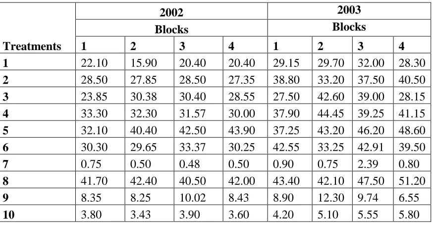
Example 1: Here yield data on wheat for 2003 data is taken for the Bayesian analysis which serves the purpose of providing the likelihood information and the 2002 data serves the purpose of providing the prior information. The analysis is done in SAS package (SAS, 1990) in Interactive Matrix Language (IML). SAS codes are available with the authors and can be obtained on request. First we carry out usual classical analysis and then Bayesian analysis is performed.
Table 2: Yield of wheat in quintal/hectare year
Treatments
2002 2003
Blocks Blocks
1 2 3 4 1 2 3 4
1 22.10 15.90 20.40 20.40 29.15 29.70 32.00 28.30
2 28.50 27.85 28.50 27.35 38.80 33.20 37.50 40.50
3 23.85 30.38 30.40 28.55 27.50 42.60 39.00 28.15
4 33.30 32.30 31.57 30.00 37.90 44.45 39.25 41.15
5 32.10 40.40 42.50 43.90 37.25 43.20 46.20 48.60
6 30.30 29.65 33.37 30.25 42.55 33.25 42.91 39.50
7 0.75 0.50 0.48 0.50 0.90 0.75 2.39 0.80
8 41.70 42.40 40.50 42.00 43.40 42.10 47.50 51.20
9 8.35 8.25 10.02 8.43 8.90 12.30 9.74 6.55
Classical Analysis
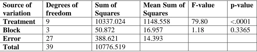
We first conducted usual (classical) analysis of the data. The analysis of variance table is given in Table 3.
Table 3: Analysis of variance with the original 2003 data
Source of variation
Degrees of freedom
Sum of Squares
Mean Sum of Squares
F-value p-value
Treatment 9 10337.024 1148.558 79.80 <.0001
Block 3 50.872 16.957 1.18 0.3365
Error 27 388.621 14.393
Total 39 10776.519
From the table it is observed that the treatment effects are significant at 5% level of significance and block effects are not significant at 5% level of significance. We then performed the test for pair wise comparison, i.e., whether there is any significance difference between a pair of treatment effects or not. Under this pair wise treatment effects comparison it is found that there are 12 number of treatment pairs which are not significant and these are (1,3), (2,3), (2,4), (2,6), (3,6), (4,5), (4,6), (4,8), (5,6), (5,8), (7,10) and (9,10). For example, treatment 1 is not significantly different from treatment 3 for the treatment comparison (1, 3) and so on.
Bayesian analysis
for F (= 0.05, 3, 27) is 2.96. We then carry out testing for individual treatment effects comparisons. It was found that 7 treatment pairs are non significant. These pairs are (2,3), (2,4), (2,6), (4,5), (4,6), (5,8), and (7,10).
There are 12 treatment pairs which are not significant in classical method of analysis. On performing Bayesian analysis of the same set of data and combining the related prior information in the procedure of analysis there are only 7 non-significant pairs of treatment effects under Normal-Gamma prior. Thus we find improvement over 5 treatment pairs. These pairs are (1,3), (3,6), (4,8), (5,6) and (9,10 ), i.e., these treatment pairs are now significant under Bayesian analysis.
Example 2: Here the data for the year 1999 on wheat is considered as data providing prior information while the data for year 2000 is taken as current data for likelihood information.
Table 4: Yield of wheat in quintal/hectare
Treatment
1999 2000
Block Block
1 2 3 4 1 2 3 4
1 21.78 22.80 27.70 23.40 20.10 19.30 18.60 20.30
2 37.40 32.10 40.20 35.55 30.00 28.10 32.85 32.95
3 35.50 34.80 40.85 39.80 29.40 33.35 36.30 37.40
4 36.45 34.10 39.40 37.10 30.15 33.25 34.25 39.10
5 40.90 44.80 41.10 39.35 43.40 40.80 41.10 38.90
6 30.80 32.95 28.00 28.83 30.40 24.60 30.85 32.65
7 1.85 1.25 1.23 1.65 1.95 1.10 1.25 1.80
8 40.10 42.10 40.00 47.70 32.80 38.80 41.50 43.90
9 19.20 20.88 19.35 11.38 15.60 13.75 14.87 13.55
10 3.90 3.60 5.10 2.90 3.40 3.95 4.90 3.40
Table 5: Analysis of variance with the original year 2000 data
Source of variation
Degrees of freedom
Sum of Squares
Mean Sum of Squares
F-value p-value
Treatment 9 7286.691 809.632 134.97 <.0001
Block 3 56.206 18.735 3.12 0.0423
Error 27 161.967 5.998
Total 39 7504.865
Bayesian analysis
We find that the F-test value in case of Normal-Gamma prior for the treatment effects is 199.2010, while tabulated value for F (=0.05, 9, 27) is 2.2501. Therefore treatment effects are significant at 5% level of significance. The block effects are also found to be significant, as the F-test value for the block effects is 5.6264, while tabulated value for F (=0.05, 3, 27) is 2.9603. Under pair wise comparison of treatment effects we found that pairs (2,3) and (2,4) have now become significant. However, pairs (2,6), (3,4), (5,8) and (7,10) are still not significant. Thus there is a significant change is observed in using Bayesian methods.
5. Discussion
In the present study we present the Bayesian methodologies for analyzing experimental data. Here we restricted ourselves to the case of conjugate prior distributions of the parameters. Bayesian methods are well established in general linear models, where the design matrix is of full column rank. Here the approach is taken as that of Broemeling (1985), who developed usual F-statistics and t-statistic for testing the parameters or a linear function of parameters. However, these methods cannot be applied directly to designed experiments, because of rank deficiency of its design matrix. Therefore, reparameterization has been done in order to obtain full rank model.
One point to note is that though we need prior information for the parameters, yet one may wonder how old this prior information should be. For application in the present study, we had a series of experiments. Analysis was done by taking the data for a particular year and the data corresponding to its previous year was taken as prior information. However, we have also analyzed a data set for a particular year by taking a long series of data of previous years as prior separately. But there is not much change in the results as compared to that obtained by taking just previous year’s data as prior. This suggests that for analyzing data from Bayesian point of view we need only the previous information about the parameters, it does not matter how old that information is.
References
1. Berger, J. O. (1985). Statistical decision theory and Bayesian analysis (Second edition). Springer–Verlag, New York:
2. Box, G. E .P. and Tiao, G.C. (1973). Bayesian inference in statistical analysis.
Addison-Wesley Publishing Company, London.
3. Broemeling, L. D. (1985). Bayesian analysis of linear models. Marcel Dekker, New York.
4. Chaloner, K. and Verdinelli, I. (1995). Bayesian experimental design: A review,
Statistical Science, 10, 273 – 304.
6. Etzione, R. and Kadane, J. B. (1993). Optimal experimental design for another’s analysis. J. Amer. Statist. Assoc., 88, 1404-1411.
7. Flournoy, N. (1993). A clinical experiment in bone marrow transplantation: estimating a percentage point of a quantal response curve. In case studies in Bayesian Statistics, 324-336, Springer, New York.
8. Graybill, F. A. (1961). An introduction to linear statistical models. McGraw Hill, New York.
9. Lindley, D. V. and Singpurwalla, N. D. (1991). On the evidence needed to reach agreed action between adversaries, with application to acceptance sampling, J. A. S. A., 86, 933-937.
10. Raiffa, H. and Schlaifer, R. (1961). Applied statistical decision theory. Harvard University Press. Cambridge.
11. SAS Institute Inc. (1989). SAS/STAT User’s Guide, Vol.2, version 6, 4th ed. Cary, NC.
12. Savage, L.J. (1972). The foundation of statistics. Dover, Inc., New York.
13. Tsutkawa, R. K. (1972). Design of an experiment for Bio assay. J. Amer. Statist. Assoc. 67, 584-590.