Transmuted Complementary Weibull Geometric Distribution

Ahmed Z. Afify

Department of Statistics, Mathematics and Insurance Benha University, Egypt

[email protected]

Zohdy M. Nofal

Department of Statistics, Mathematics and Insurance Benha University, Egypt

[email protected]

Nadeem Shafique Butt

Department of Statistics, COMSATS Institute of Information Technology Lahore, Pakistan

[email protected]

Abstract

This paper provides a new generalization of the complementary Weibull geometric distribution introduced by Tojeiro et al. (2014), using the quadratic rank transmutation map studied by Shaw and Buckley (2007). The new distribution is referred to as transmuted complementary Weibull geometric distribution (TCWGD). The TCWG distribution includes as special cases 11 sub models such as the complementary Weibull geometric distribution (CWGD), complementary exponential geometric distribution (CEGD), Weibull distribution (WD), exponential distribution (ED) and three new submodels. Various structural properties of the new distribution including moments, quantiles, moment generating function and Rényi entropy of the subject distribution are derived. We proposed the method of maximum likelihood for estimating the model parameters. Two real data sets are used to compare the flexibility of the new model versus the complementary Weibull geometric distribution.

Keywords: Transmutation, complementary Weibull geometric, Reliability Function, Moment Generating Function, Rényi Entropy, Order Statistics, Maximum Likelihood Estimation.

1. Introduction

The Weibull distribution is of utmost interest to theory-orientated statisticians because of its great number of special features and to practitioners because of its ability to fit to data from various fields, ranging from life data to observations made in economics and business administration, meteorology, hydrology, maintenance, replacement, quality control, acceptance sampling, statistical process control, inventory control, geology, geography, astronomy, medicine, psychology, pharmacy, material science, engineering, physics, chemistry, biology, warranty and weather data, see, e.g., Rinne (2009). For more than half a century the Weibull distribution has attracted the attention of statisticians working on theory and methods as well as in various fields of applied statistics.

transmuted Weibull distribution. Khan and King (2013) introduced the transmuted modified Weibull distribution. Ashour and Eltehiwy (2013a, 2013b) studied the transmuted exponentiated modi.ed Weibull and transmuted exponentiated Lomax distributions. Ebraheim (2014) introduced exponentiated transmuted Weibull distribution.

An interesting idea of generalizing a distribution, known in the literature by transmution, is derived by using the quadratic rank transmutation map studied by Shaw and Buckley (2007). In this paper we propose a new distribution family by extending the complementary Weibull geometric (CWG), introduced by Tojeiro et al. (2014) by using the quadratic rank transmutation map.

Louzada et al. (2011) introduced the complementary exponential geometric distribution, which is complementary to the exponential geometric model proposed by Adamidis and Loukas (1998), based on a complementary risk problem (Basu and J., 1982) in presence of latent risks, in the sense that there is no information about which factor was responsible for the component failure but only the maximum lifetime value among all risks is observed. Louzada et al. (2013) introduced complementary exponentiated exponential geometric distribution which considered a generalization to the complementary exponential geometric distribution. Tojeiro et al. (2014) introduced the complementary Weibull geometric (CWG) as a complementary distribution to the Weibull geometric (WG) model proposed by Barreto-Souza et al. (2011).

The cumulative distribution function (𝑐𝑑𝑓) of the complementary Weibull geometric distribution (CWGD) is given by

𝐹𝐶𝑊𝐺(𝑦, 𝛼, 𝛽, 𝛾) =

𝛼(1−𝑒−(𝛾𝑦)𝛽₎

𝛼+(1−𝛼)𝑒−(𝛾𝑦)𝛽, 𝑦, 𝛼, 𝛽, 𝛾 > 0, (1)

where 𝛾 is a scale parameter and 𝛼and 𝛽 are shape parameters. The corresponding probability density function (𝑝𝑑𝑓) is given by

𝑓_𝐶𝑊𝐺(𝑦, 𝛼, 𝛽, 𝛾) =𝛼𝛽𝛾(𝛾𝑦)𝛽−1𝑒−(𝛾𝑦)𝛽

(𝛼+(1−𝛼)𝑒−(𝛾𝑦)𝛽₎2. (2)

The procedure of expanding a family of distributions for added flexibility or to construct covariate models is a well-known technique in the literature. In this article we present a new generalization of complementary Weibull geometric distribution called transmuted complementary Weibull geometric distribution. We derived the subject distribution using the quadratic rank transmutation map studied by Shaw and Buckley (2007). A random variable 𝑋 is said to have transmuted distribution if its cumulative distribution function (𝑐𝑑𝑓) is given by

𝐹(𝑥) = (1 + 𝜆)𝐺(𝑥) − 𝜆𝐺2_{(𝑥), |𝜆| ≤ 1.}

where 𝑓(𝑥) and 𝑔(𝑥) are the corresponding 𝑝𝑑𝑓𝑠 associated with 𝑐𝑑𝑓𝑠 𝐹(𝑥) and 𝐺(𝑥) respectively. For more information about the quadratic rank transmutation map is given in Shaw and Buckley (2007). Observe that at 𝜆 = 0, we have the base distribution.

In this paper we provide mathematical formulation of the transmuted complementary Weibull geometric distribution (TCWGD) and some of its properties. We will also provide possible area of applications. The rest of the paper is organized as follows. In Section 2 we demonstrate the subject distribution. In Section 3, we find the reliability function, hazard rate and cumulative hazard rate of the subject model. The statistical properties include quantile functions, random number generation, moments, moment generating functions and Rényi entropy are derived in Section 4. In section 5, the minimum, maximum and median order statistics models are discussed. We also demonstrate the joint density functions 𝑓_{𝑖:𝑗;𝑛}(𝑥_𝑖, 𝑥_𝑗) of the transmuted complementary Weibull geometric distribution. In Section 6, we demonstrate the maximum likelihood estimates (MLEs) and the asymptotic confidence intervals of the unknown parameters. In section 7, the TCWG distribution is applied to a real data set to illustrate its usefulness. Finally, in Section 8, we provide some concluding remarks.

2. Transmuted Complementary Weibull Geometric Distribution (TCWGD)

The transmuted complementary Weibull geometric distribution (TCWGD) and its sub-models are presented in this section. A random variable 𝑌 is said to have transmuted complementary Weibull geometric distribution with parameters 𝛼, 𝛽, 𝛾 and 𝛿 if its cumulative distribution function (𝑐𝑑𝑓) is defined as

𝐹_{𝑇𝐶𝑊𝐺}(𝑦, 𝛼, 𝛽, 𝛾, 𝛿) =𝛼

2_{+ ((𝛼𝛿 + 𝛼 − 2𝛼}2_{) − (𝛼𝛿 + 𝛼 − 𝛼}2_)𝑒−(𝛾𝑦)𝛽

) 𝑒−(𝛾𝑦)𝛽

(𝛼 + (1 − 𝛼)𝑒−(𝛾𝑦)𝛽₎2 ,

𝑦 > 0, 𝛼, 𝛽, 𝛾 > 0, |𝛿| ≤ 1. (3)

Using the series expansion

(1 − 𝑍)−𝑘 _{= ∑}Γ(𝑘 + 𝑗)

𝑗! Γ(𝑘)

∞

𝑗=0

𝑍𝑗_{, 0 < 𝑍 < 1, 𝑘 > 0.}

The 𝑐𝑑𝑓 of the transmuted complementary Weibull geometric in (3) can be expressed in the mixture form

𝐹_{𝑇𝐶𝑊𝐺}(𝑦, 𝛼, 𝛽, 𝛾, 𝛿) = ∑∞ (𝑗 + 1) (1 −_𝛼1)𝑗𝑒−𝑗(𝛾𝑦)𝛽 𝑗=0

+_𝛼ℎ₂∑ ∑ (−1)𝑖(𝑗+2)

Γ(2−𝑖)𝑖!𝑗! ℓ

𝑗_{(1 −}1 𝛼)

𝑗

𝑒−(𝑖+𝑗+1)(𝛾𝑦)𝛽

∞ 𝑗=0 ∞

𝑖=0 .

(4)

is the transmuted parameter. The corresponding probability density function (𝑝𝑑𝑓) of the transmuted complementary Weibull geometric distribution is given by

𝑓_{𝑇𝐶𝑊𝐺}(𝑦, 𝛼, 𝛽, 𝛾, 𝛿) =𝛼𝛽𝛾(𝛾𝑦)𝛽−1𝑒−(𝛾𝑦)𝛽(𝛼(1−𝛿)−(𝛼−𝛼𝛿−𝛿−1)𝑒−(𝛾𝑦)𝛽)

(𝛼+(1−𝛼)𝑒−(𝛾𝑦)𝛽₎3 . (5)

Using the series expansion the 𝑝𝑑𝑓 of the transmuted complementary Weibull geometric distribution in (5) can be expressed in the mixture form

𝑓_{𝑇𝐶𝑊𝐺}(𝑦, 𝛼, 𝛽, 𝛾, 𝛿) =𝛽𝛾(1−𝛿)_2𝛼 (𝛾𝑦)𝛽−1_{∑ ∑} (−1)𝑖Γ(𝑗+3)

Γ(2−𝑖)𝑖!𝑗! 𝑘𝑖(1 − ∞

𝑗=0 ∞ 𝑖=0 1

𝛼) 𝑗

𝑒−(𝑖+𝑗+1)(𝛾𝑦)𝛽_{. (6)}

where 𝑘 = (𝛼 − 𝛼𝛿 − 𝛿 − 1)/𝛼(1 − 𝛿), 𝛿 ≠ 1.

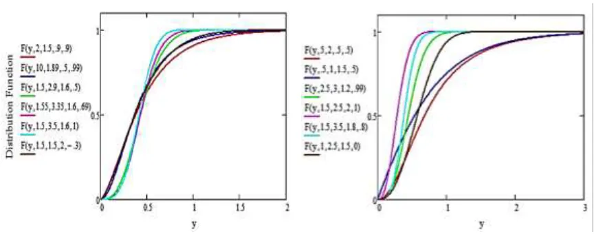
Figures 1 and 2 show some of the possible shapes of the𝑝𝑑𝑓 and 𝑐𝑑𝑓of TCWGD for different choices of the parameters 𝛼, 𝛽, 𝛾 and 𝛿 respectively.

Figure 1: Probability Density Function of the TCWGD

The transmuted complementary Weibull geometric distribution is very flexible model that approaches to different distributions when its parameters are changed. The subject distribution contains 11 sub models of well known and unknown probability distributions, as special cases, such as the transmuted complementary exponential geometric distribution (TCEGD), the transmuted complementary Rayleigh geometric distribution (TCRGD) and the complementary Rayleigh geometric distributio (CRGD). These three sub models are new distributions. The flexibility of the transmuted complementary Weibull geometric distribution is illustrated in the following .

Corollary 1 If 𝑌 is a random variable with 𝑝𝑑𝑓 in (5), then we have the following special cases.

1. When 𝛿 = 0, we get the complementary Weibull geometric distribution, CWGD(𝛼, 𝛽, 𝛾, 𝑦).

2. When 𝛽 = 1, we get the transmuted complementary exponential geometric distribution, TCEGD(𝛼, 𝛾, 𝛿, 𝑦). (New)

3. When 𝛽 = 2, we get the transmuted complementary Rayleigh geometric distribution, TCRGD(𝛼, 𝛾, 𝛿, 𝑦). (New)

4. When 𝛽 = 1 and 𝛿 = 0, we get the complementary exponential geometric distribution, CEGD(𝛼, 𝛾, 𝑦).

5. When 𝛽 = 2 and 𝛿 = 0, we get the complementary Rayleigh geometric distribution, CRGD(𝛼, 𝛾, 𝑦). (New)

6. When 𝛼 = 1, we get the transmuted Weibull distribution, TWD(𝛽, 𝛾, 𝛿, 𝑦). 7. When 𝛼 = 1 and 𝛿 = 0, we get the Weibull geometric distribution, WD(𝛽, 𝛾, 𝑦). 8. When 𝛼 = 𝛽 = 1, we get the transmuted exponential distribution, TED(𝛾, 𝛿, 𝑦). 9. When 𝛼 = 𝛽 = 1, and 𝛿 = 0, we get the exponential distribution, ED(𝛾, 𝑦). 10. When 𝛼 = 1 and 𝛽 = 2, we get the transmuted Rayleigh distribution,

TRD(𝛾, 𝛿, 𝑦).

11. When 𝛼 = 1, 𝛽 = 2, and 𝛿 = 0, we get the Rayleigh distribution, RD(𝛾, 𝑦).

3. Reliability Analysis

The characteristics in reliability analysis which are the reliability function (RF), the hazard rate function (HF), the cumulative hazard rate function (CHF) for the TCWGD(𝛼, 𝛽, 𝛾, 𝛿, 𝑦) are introduced in this section.

3.1 Reliability Function

The reliability function (𝑅𝐹) also known as the survival function, which is the probability of an item not failing prior to some time 𝑡, is defined by 𝑅(𝑦) = 1 − 𝐹(𝑦). The reliability function of the transmuted complementary Weibull geometric distribution denoted by 𝑅𝑇𝐶𝑊𝐺(𝑦, 𝛼, 𝛽, 𝛾, 𝛿), can be a useful characterization of life time data

analysis. It can be defined as 𝑅𝑇𝐶𝑊𝐺(𝑦, 𝛼, 𝛽, 𝛾, 𝛿) = 1 − 𝐹𝑇𝐶𝑊𝐺(𝑦, 𝛼, 𝛽, 𝛾, 𝛿),

𝑅_{𝑇𝐶𝑊𝐺}(𝑦, 𝛼, 𝛽, 𝛾, 𝛿) =(𝛼(1−𝛿)−(𝛼−𝛼𝛿−1)𝑒−(𝛾𝑦)𝛽)𝑒−(𝛾𝑦)𝛽

Using the series expansion the 𝑅𝐹 of the transmuted complementary Weibull geometric distribution in (7) can be expressed in the mixture form as follows

𝑅_{𝑇𝐶𝑊𝐺}(𝑦, 𝛼, 𝛽, 𝛾, 𝛿) =1−𝛿_𝛼 ∑ ∑ (−1)_{Γ(2−𝑖)𝑖!}𝑖(𝑗+1)𝑝𝑖_{(1 −}1 𝛼)

𝑗

𝑒−(𝑖+𝑗+1)(𝛾𝑦)𝛽 ∞

𝑗=0 ∞

𝑖=0 . (8)

where 𝑝 = (𝛼 − 𝛼𝛿 − 1)/𝛼(1 − 𝛿), 𝛿 ≠ 1.

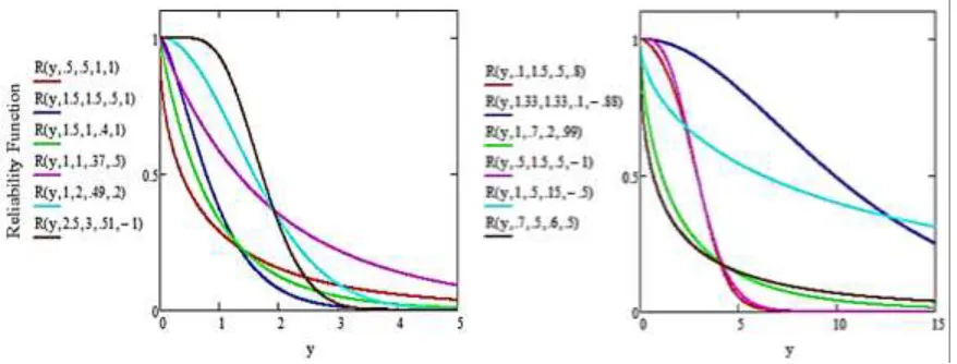
Figure 3 illustrates the pattern of the transmuted complementary Weibull geometric distribution reliability function with different choices of parameters 𝛼, 𝛽, 𝛾 and 𝛿.

Figure 3: Reliability Function of the TCWGD

3.2 Hazard Rate Function

The other characteristic of interest of a random variable is the hazard rate function (𝐻𝐹).The hazard function of the transmuted complementary Weibull geometric distribution also known as instantaneous failure rate denoted by ℎ𝑇𝐶𝑊𝐺(𝑦), is an

important quantity characterizing life phenomenon. It can be loosely interpreted as the conditional probability of failure, given it has survived to the time 𝑡. The 𝐻𝐹 of the transmuted complementary Weibull geometric distribution is defined by ℎ_{𝑇𝐶𝑊𝐺}(𝑦, 𝛼, 𝛽, 𝛾, 𝛿) = 𝑓_{𝑇𝐶𝑊𝐺}(𝑦, 𝛼, 𝛽, 𝛾, 𝛿)/𝑅_{𝑇𝐶𝑊𝐺}(𝑦, 𝛼, 𝛽, 𝛾, 𝛿),

ℎ_{𝑇𝐶𝑊𝐺}(𝑦, 𝛼, 𝛽, 𝛾, 𝛿) = 𝛼𝛽𝛾(𝛾𝑦)𝛽−1𝑒−(𝛾𝑦)𝛽(𝛼(1−𝛿)+(1−𝛼+𝛼𝛿+𝛿)𝑒−(𝛾𝑦)𝛽)

(𝛼+(1−𝛼)𝑒−(𝛾𝑦)𝛽_{)(𝛼(1−𝛿)𝑒}−(𝛾𝑦)𝛽_{+(1−𝛼+𝛼𝛿)𝑒}−2(𝛾𝑦)𝛽₎. (9)

Using the series expansion, the 𝐻𝐹 of the transmuted complementary Weibull geometric distribution in (9) can be expressed in the mixture form as follows

ℎ𝑇𝐶𝑊𝐺(𝑦, 𝛼, 𝛽, 𝛾, 𝛿) = 𝛽𝛾(𝛾𝑦)𝛽−1

∑ ∑ (−1)𝑖Γ(𝑗+3)_{Γ(2−𝑖)𝑖!𝑗!} 𝑘𝑖₍₁₋1 𝛼)

𝑗

𝑒−(𝑖+𝑗+1)(𝛾𝑦)𝛽 ∞

𝑗=0 ∞ 𝑖=0

2 ∑ ∑ (−1)𝑖(𝑗+1)

Γ(2−𝑖)𝑖! 𝑝𝑖(1− 1 𝛼)

𝑗

𝑒−(𝑖+𝑗+1)(𝛾𝑦)𝛽 ∞

𝑗=0 ∞ 𝑖=0

. (10)

Figure 4 illustrates some of the possible shapes of the hazard rate function of the transmuted complementary Weibull geometric distribution for different values of the parameters𝛼, 𝛽, 𝛾 and 𝛿.

Figure 4: Hazard Rate of the TEFD

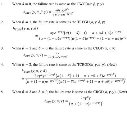
Corollary 2 The hazard rate function of the transmuted complementary Weibull geometric distribution TCWGD(𝛼, 𝛽, 𝛾, 𝛿, 𝑦) has the following special cases

1. When 𝛿 = 0, the failure rate is same as the CWGD(𝛼, 𝛽, 𝛾, 𝑦)

ℎ𝐶𝑊𝐺(𝑦, 𝛼, 𝛽, 𝛾) = 𝛼𝛽𝛾(𝛾𝑦)

𝛽−1

𝛼+(1−𝛼)𝑒−(𝛾𝑦)𝛽.

2. When 𝛽 = 1, the failure rate is same as the TCEGD(𝛼, 𝛾, 𝛿, 𝑦). ℎ_{𝑇𝐶𝐸𝐺}(𝑦, 𝛼, 𝛾, 𝛿)

= 𝛼𝛾𝑒−(𝛾𝑦)(𝛼(1 − 𝛿) + (1 − 𝛼 + 𝛼𝛿 + 𝛿)𝑒−(𝛾𝑦))

(𝛼 + (1 − 𝛼)𝑒−(𝛾𝑦)_{)(𝛼(1 − 𝛿)𝑒}−(𝛾𝑦)_{+ (1 − 𝛼 + 𝛼𝛿)𝑒}−2(𝛾𝑦)₎.

3. When 𝛽 = 1 and 𝛿 = 0, the failure rate is same as the CEGD(𝛼, 𝛾, 𝑦) ℎ_𝐶𝐸𝐺(𝑦, 𝛼, 𝛾) =_{𝛼+(1−𝛼)𝑒}𝛼𝛾 _{−(𝛾𝑦)}.

4. When 𝛽 = 2, the failure rate is same as the TCRGD(𝛼, 𝛾, 𝛿, 𝑦). (New) ℎ_{𝑇𝐶𝑅𝐺}(𝑦, 𝛼, 𝛾, 𝛿)

= 2𝛼𝛾2y𝑒−(𝛾𝑦)

2

(𝛼(1 − 𝛿) + (1 − 𝛼 + 𝛼𝛿 + 𝛿)𝑒−(𝛾𝑦)2₎

(𝛼 + (1 − 𝛼)𝑒−(𝛾𝑦)2_{)(𝛼(1 − 𝛿)𝑒−(𝛾𝑦)}2 _{+ (1 − 𝛼 + 𝛼𝛿)𝑒−2(𝛾𝑦)}2₎.

5. When 𝛽 = 2 and 𝛿 = 0, the failure rate is same as the CRGD(𝛼, 𝛾, 𝑦). (New)

ℎ𝐶𝑅𝐺(𝑦, 𝛼, 𝛾) =

2𝛼𝛾2_y

6. When 𝛼 = 1, the failure rate is same as the TWD(𝛽, 𝛾, 𝛿, 𝑦).

ℎ_𝑇𝑊(𝑦, 𝛽, 𝛾, 𝛿) =𝛽𝛾(𝛾𝑦)

𝛽−1_𝑒−(𝛾𝑦)𝛽

((1 − 𝛿) + 2𝛿𝑒−(𝛾𝑦)𝛽

)

((1 − 𝛿)𝑒−(𝛾𝑦)𝛽_{+ 𝛿𝑒−2(𝛾𝑦)}𝛽₎ .

7. When 𝛼 = 1 and 𝛿 = 0, the failure rate is same as the WD(𝛽, 𝛾, 𝑦). ℎ𝑊(𝑦, 𝛽, 𝛾) = 𝛽𝛾(𝛾𝑦)𝛽−1.

8. When 𝛼 = 𝛽 = 1, the failure rate is same as the TED(𝛾, 𝛿, 𝑦).

ℎ𝑇𝐸(𝑦, 𝛾, 𝛿) =

𝛾𝑒−(𝛾𝑦)_{((1 − 𝛿) + 2𝛿𝑒}−(𝛾𝑦)₎

((1 − 𝛿)𝑒−(𝛾𝑦)_{+ 𝛿𝑒}−2(𝛾𝑦)₎ .

9. When 𝛼 = 𝛽 = 1, and 𝛿 = 0, the failure rate is same as the ED(𝛾, 𝑥). ℎ𝐸(𝑦, 𝛾) = 𝛾.

10. When 𝛼 = 1 and 𝛽 = 2, the failure rate is same as the TRD(𝛾, 𝛿, 𝑦).

ℎ𝑇𝑅(𝑦, 𝛾, 𝛿) =

2𝛾2_y𝑒−(𝛾𝑦)2

((1 − 𝛿) + 2𝛿𝑒−(𝛾𝑦)2

)

((1 − 𝛿)𝑒−(𝛾𝑦)2 _{+ 𝛿𝑒−2(𝛾𝑦)}2₎ .

11. When 𝛼 = 1, 𝛽 = 2, and 𝛿 = 0, the failure rate is same as the RD(𝛾, 𝑦).

ℎ_𝑅(𝑦, 𝛾) = 2𝛾2_y.

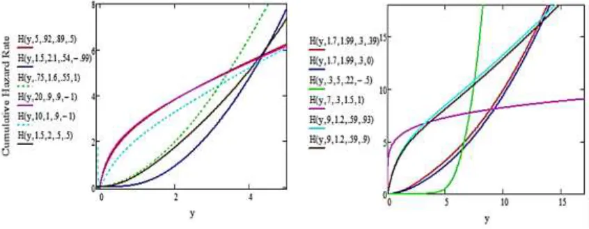
3.3 Cumulative Hazard Rate Function

The Cumulative hazard function (𝐶𝐻𝐹) of the transmuted complementary Weibull geometric distribution, denoted by 𝐻_{𝑇𝐶𝑊𝐺}(𝑦, 𝛼, 𝛽, 𝛾, 𝛿), is defined as

𝐻_{𝑇𝐶𝑊𝐺}(𝑦, 𝛼, 𝛽, 𝛾, 𝛿) = ∫

𝑥

0

ℎ_{𝑇𝐶𝑊𝐺}(𝑦, 𝛼, 𝛽, 𝛾, 𝛿)𝑑𝑥 = −ln𝑅_{𝑇𝐶𝑊𝐺}(𝑦, 𝛼, 𝛽, 𝛾, 𝛿),

𝐻_{𝑇𝐶𝑊𝐺}(𝑦, 𝛼, 𝛽, 𝛾, 𝛿) = ln ( (𝛼+(1−𝛼)𝑒−(𝛾𝑦)𝛽)

2

𝛼(1−𝛿)𝑒−(𝛾𝑦)𝛽_{+(1−𝛼+𝛼𝛿)𝑒}−2(𝛾𝑦)𝛽). (11)

We can express the 𝐶𝐻𝐹 of the TCWGD using the series expansion as follows

𝐻_{𝑇𝐶𝑊𝐺}(𝑦, 𝛼, 𝛽, 𝛾, 𝛿) = −ln (1−𝛿_𝛼 ∑ ∑ (−1)𝑖(𝑗+1)

Γ(2−𝑖)𝑖! 𝑝

𝑖_{(1 −}1 𝛼)

𝑗

𝑒−(𝑖+𝑗+1)(𝛾𝑦)𝛽

∞ 𝑗=0 ∞

𝑖=0 ). (12)

where ℓ is defined above. It is important to note that the units for 𝐻𝑇𝐶𝑊𝐺(𝑦, 𝛼, 𝛽, 𝛾, 𝛿) is

the cumulative probability of failure or death per unit of time, distance or cycles.

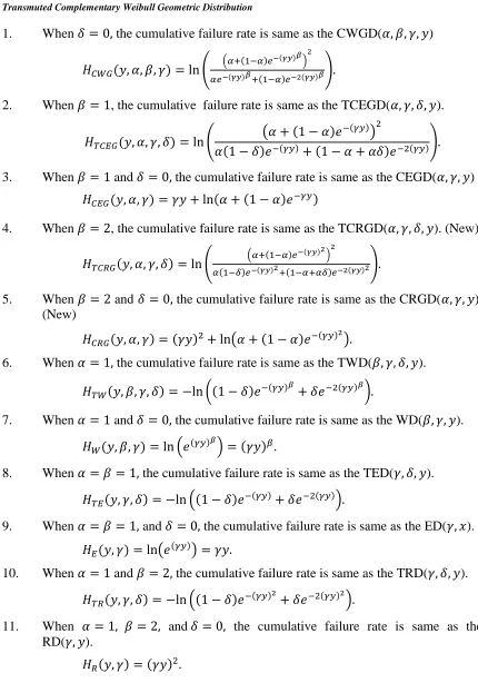
1. When 𝛿 = 0, the cumulative failure rate is same as the CWGD(𝛼, 𝛽, 𝛾, 𝑦)

𝐻_𝐶𝑊𝐺(𝑦, 𝛼, 𝛽, 𝛾) = ln ( (𝛼+(1−𝛼)𝑒−(𝛾𝑦)𝛽)

2

𝛼𝑒−(𝛾𝑦)𝛽_{+(1−𝛼)𝑒}−2(𝛾𝑦)𝛽).

2. When 𝛽 = 1, the cumulative failure rate is same as the TCEGD(𝛼, 𝛾, 𝛿, 𝑦).

𝐻_{𝑇𝐶𝐸𝐺}(𝑦, 𝛼, 𝛾, 𝛿) = ln ( (𝛼 + (1 − 𝛼)𝑒−(𝛾𝑦))

2

𝛼(1 − 𝛿)𝑒−(𝛾𝑦)_{+ (1 − 𝛼 + 𝛼𝛿)𝑒}−2(𝛾𝑦)).

3. When 𝛽 = 1 and 𝛿 = 0, the cumulative failure rate is same as the CEGD(𝛼, 𝛾, 𝑦) 𝐻_𝐶𝐸𝐺(𝑦, 𝛼, 𝛾) = 𝛾𝑦 + ln(𝛼 + (1 − 𝛼)𝑒−𝛾𝑦₎

4. When 𝛽 = 2, the cumulative failure rate is same as the TCRGD(𝛼, 𝛾, 𝛿, 𝑦). (New)

𝐻_{𝑇𝐶𝑅𝐺}(𝑦, 𝛼, 𝛾, 𝛿) = ln ( (𝛼+(1−𝛼)𝑒−(𝛾𝑦)2)

2

𝛼(1−𝛿)𝑒−(𝛾𝑦)2_{+(1−𝛼+𝛼𝛿)𝑒}−2(𝛾𝑦)2).

5. When 𝛽 = 2 and 𝛿 = 0, the cumulative failure rate is same as the CRGD(𝛼, 𝛾, 𝑦). (New)

𝐻_𝐶𝑅𝐺(𝑦, 𝛼, 𝛾) = (𝛾𝑦)2_{+ ln(𝛼 + (1 − 𝛼)𝑒}−(𝛾𝑦)2_).

6. When 𝛼 = 1, the cumulative failure rate is same as the TWD(𝛽, 𝛾, 𝛿, 𝑦).

𝐻𝑇𝑊(𝑦, 𝛽, 𝛾, 𝛿) = −ln ((1 − 𝛿)𝑒−(𝛾𝑦)𝛽 + 𝛿𝑒−2(𝛾𝑦)𝛽).

7. When 𝛼 = 1 and 𝛿 = 0, the cumulative failure rate is same as the WD(𝛽, 𝛾, 𝑦).

𝐻_𝑊(𝑦, 𝛽, 𝛾) = ln (𝑒(𝛾𝑦)𝛽

) = (𝛾𝑦)𝛽_.

8. When 𝛼 = 𝛽 = 1, the cumulative failure rate is same as the TED(𝛾, 𝛿, 𝑦).

𝐻𝑇𝐸(𝑦, 𝛾, 𝛿) = −ln ((1 − 𝛿)𝑒−(𝛾𝑦)+ 𝛿𝑒−2(𝛾𝑦)).

9. When 𝛼 = 𝛽 = 1, and 𝛿 = 0, the cumulative failure rate is same as the ED(𝛾, 𝑥). 𝐻_𝐸(𝑦, 𝛾) = ln(𝑒(𝛾𝑦)_{) = 𝛾𝑦.}

10. When 𝛼 = 1 and 𝛽 = 2, the cumulative failure rate is same as the TRD(𝛾, 𝛿, 𝑦).

𝐻𝑇𝑅(𝑦, 𝛾, 𝛿) = −ln ((1 − 𝛿)𝑒−(𝛾𝑦)2 + 𝛿𝑒−2(𝛾𝑦)2).

11. When 𝛼 = 1, 𝛽 = 2, and 𝛿 = 0, the cumulative failure rate is same as the RD(𝛾, 𝑦).

𝐻_𝑅(𝑦, 𝛾) = (𝛾𝑦)2_.

Figure 5: Cumulative Hazard Rate of the TCWGD

4. Statistical properties

The statistical properties of the transmuted complementary Weibull geometric distribution including quantile and random number generation, moments, moment generating function and Rényi entropy are discussed in this section.

4.1 Quantile and Median

The quantile 𝑦_𝑞 of the transmuted complementary Weibull geometric distribution TCWGD(𝛼, 𝛽, 𝛾, 𝛿, 𝑦) is the real solution of the following equation 𝐹(𝑦_𝑞) = 𝑞, and is given by the following

𝑦𝑞 = 𝛾−1{ln (−𝑘+𝛼√1+𝛿(𝛿−4𝑞+2)_2𝛼2_(1−𝑞) )}

1/𝛽

, 0 ≤ 𝑞 ≥ 1, (13)

where 𝑘 = 2𝛼𝑞(𝛼 − 1) − 2𝛼2_{+ 𝛼(1 + 𝛿).}

If we put 𝑞 = 0.5 in the above equation we can get the median of the TCWGD(𝛼, 𝛽, 𝛾, 𝛿, 𝑦). The quantile 𝑦𝑞 of the transmuted complementary Weibull

geometric distribution. The median life of the subject distribution is the 50-th percentile. In practice, this is the life by which 50 percent of the units will be expected to have failed and so it is the life at which 50 percent of the units would be expected to still survive.

4.2 Random Number Generation

The random number 𝑦 of the TCWGD(𝛼, 𝛽, 𝛾, 𝛿, 𝑦) is defined by the following relation 𝐹𝑇𝐶𝑊𝐺(𝑦, 𝛼, 𝛽, 𝛾, 𝛿) = 𝜁, where 𝜁~ 𝑈(0,1), then

𝛼2_{+ ((𝛼𝛿 + 𝛼 − 2𝛼}2_{) − (𝛼𝛿 + 𝛼 − 𝛼}2_)𝑒−(𝛾𝑦)𝛽

) 𝑒−(𝛾𝑦)𝛽

(𝛼 + (1 − 𝛼)𝑒−(𝛾𝑦)𝛽₎2 = 𝜁.

Solving for 𝑦,we get

𝑦 = 𝛾−1_{{ln (}2𝛼2−2𝛼𝑞(𝛼−1)−𝛼(1+𝛿)+𝛼√1+𝛿(𝛿−4𝑞+2)

2𝛼2_(1−𝑞) )}

1/𝛽

Using a random number uniformly distributed from zero to one, we have solved the above equation to obtain a random number in 𝑦.

4.3 Moments

The 𝑟𝑡ℎ _{moment, denoted by 𝜇} 𝑟

′_{,of the TCWGD(𝛼, 𝛽, 𝛾, 𝛿, 𝑦) is given by the following}

theorem.

Theorem 1. If 𝑌 is a continuous random variable has the TCWGD(𝛼, 𝛽, 𝛾, 𝛿, 𝑦) with |𝛿| ≤ 1, then the 𝑟𝑡ℎ non-central moment of 𝑌 is given as follows

𝜇_𝑟′ _{= 𝐸(𝑌}𝑟_{) =}(1−𝛿)

2𝛼𝛾𝑟Γ (1 +

𝑟

𝛽) ∑ ∑

(−1)𝑖_Γ(𝑗+3)

Γ(2−𝑖)𝑖!𝑗! 𝑘𝑖(1 − 1 𝛼)

𝑗

(𝑖 + 𝑗 +)−(1+𝑟/𝛽) ∞

𝑗=0 ∞

𝑖=0 . (15)

Proof: By definition 𝜇𝑟′ = ∫ 0 ∞ 𝑦𝑟_𝑓 𝑇𝐶𝑊𝐺(𝑥, 𝛼, 𝛽, 𝛾, 𝛿)𝑑𝑦

=𝛽𝛾𝛽_2𝛼(1−𝛿)∑ ∑ (−1)𝑖Γ(𝑗+3)

Γ(2−𝑖)𝑖!𝑗! 𝑘

𝑖_{(1 −}1 𝛼)

𝑗

∫

0 ∞

𝑦𝑟+𝛽−1_𝑒−(𝑖+𝑗+1)(𝛾𝑦)𝛽_𝑑𝑦 ∞

𝑗=0 ∞

𝑖=0 .

(16)

To compute ∫

0 ∞

𝑦𝑟+𝛽−1_𝑒−(𝑖+𝑗+1)(𝛾𝑦)𝛽_{𝑑𝑦,let 𝑡 = (𝑖 + 𝑗 + 1)(𝛾𝑦)}𝛽_{. Then 𝑦 =}1 𝛾( 𝑡 𝑖+𝑗+1) 1/𝛽 . Therefore ∫ 0 ∞

𝑦𝑟+𝛽−1_𝑒−(𝑖+𝑗+1)(𝛾𝑦)𝛽

𝑑𝑦 = (𝑖+𝑗+1)_{𝛽𝛾𝑟+𝛽}−(1+𝑟/𝛽)Γ (1 +_𝛽𝑟). (17)

By substituting from Equation (17) into Equation (16), we obtain

𝜇_𝑟′ ₌(1−𝛿)

2𝛼𝛾𝑟 Γ (1 +

𝑟

𝛽) ∑ ∑

(−1)𝑖_Γ(𝑗+3)

Γ(2−𝑖)𝑖!𝑗! 𝑘

𝑖_{(1 −}1 𝛼)

𝑗

(𝑖 + 𝑗 + 1)−(1+𝛽𝑟)

∞ 𝑗=0 ∞

𝑖=0 .

where 𝑘 = (𝛼 − 𝛼𝛿 − 𝛿 − 1)/𝛼(1 − 𝛿), 𝛿 ≠ 1. This completes the proof.

Based on the above Theorem (1) the coefficient of variation, coefficient of skewness and coefficient of kurtosis of the TCWGD(𝛼, 𝛽, 𝛾, 𝛿, 𝑦) distribution can be obtained according to the following relations

𝐶𝑉_{𝑇𝐶𝑊𝐺} = √𝜇2′ − 𝜇1′ 𝜇₁′ ,

𝐶𝑆_{𝑇𝐶𝑊𝐺} =𝜇3′ − 3𝜇2′𝜇1′ + 2(𝜇1′)3 (𝜇₂′ _{− (𝜇}

1′)2)3/2

,

and

𝐶𝐾_{𝑇𝐶𝑊𝐺} =𝜇4′ − 4𝜇3′𝜇1′ + 6𝜇2′(𝜇1′)2− 3(𝜇1′)4 (𝜇₂′ _{− (𝜇}

1

Corollary 4 Using the relation between the central moments and non-centeral moments, we can obtain the 𝑛𝑡ℎ central moment, denoted by 𝑀_𝑛, of a TCWG random variable as follows

𝑀_𝑛 = 𝐸(𝑌 − 𝜇)𝑛 _{= ∑} 𝑛

𝑟=0

(𝑛_{𝑟) (−𝜇)}𝑛−𝑟_𝐸(𝑌𝑟_),

where 𝐸(𝑌𝑟) is the on-central moments of the TCWGD(𝛼, 𝛽, 𝛾, 𝛿, 𝑦). Therefore the 𝑛𝑡ℎ central moments of the TCWGD(𝛼, 𝛽, 𝛾, 𝛿, 𝑦) is given by

𝑀_𝑛 = (1−𝛿)_2𝛼 ∑ ∑ ∑∞ (−1)_{Γ(2−𝑖)𝑖!𝑗!}𝑖+𝑛−𝑟Γ(𝑗+3)(𝑛_{𝑟) (𝜇)}𝑛−𝑟_𝛾−𝑟_𝑘𝑖 𝑗=0

∞ 𝑖=0 𝑛

𝑟=0

× (1 −1_𝛼)𝑗(𝑖 + 𝑗 + 1)−(1+𝑟/𝛽)_{Γ (1 +}𝑟 𝛽) .

(18)

where 𝑘 is mentioned above.

4.4 Moment Generating Function

The moment generating function (𝑚𝑔𝑓) of the transmuted complementary Weibull geometric distribution is given by the following theorem.

Theorem 2. If 𝑌 is a continuous random variable has the TCWGD(𝛼, 𝛽, 𝛾, 𝛿, 𝑦) with |𝛿| ≤ 1, then the moment generating function (𝑚𝑔𝑓)of 𝑌,denoted by 𝑀_𝑌(𝑡) = 𝐸(𝑒𝑡𝑌), is given as follows

𝑀𝑌(𝑡) =(1−𝛿)_2𝛼 ∑ ∑ ∑ (−1)

𝑖_Γ(𝑗+3)

Γ(2−𝑖)𝑟!𝑖!𝑗!𝑘 𝑖₍𝑡

𝛾) 𝑟

(1 −_𝛼1)𝑗(𝑖 + 𝑗 +

∞ 𝑗=0 ∞ 𝑖=0 𝑛

𝑟=0

1)−(1+𝑟/𝛽)_{Γ (1 +}𝑟

𝛽) . (19)

Proof:

By definition

𝑀_𝑌(𝑡) = ∫

0 ∞

𝑒𝑡𝑥_𝑓

𝑇𝐶𝑊𝐺(𝑥, 𝛼, 𝛽, 𝛾, 𝛿)𝑑𝑦

= ∑𝑡𝑟 𝑟!∫

0 ∞

𝑦𝑟_𝑓

𝑇𝐶𝑊𝐺(𝑥, 𝛼, 𝛽, 𝛾, 𝛿)𝑑𝑦 ∞

𝑟=0

= ∑∞ 𝑡_𝑟!𝑟𝜇_𝑟′_.

𝑟=0 (20)

By substituting from Equation (15) into Equation (20), we obtain the following

𝑀_𝑌(𝑡) =(1−𝛿)_2𝛼 ∑ ∑ ∑ (−1)_{Γ(2−𝑖)𝑟!𝑖!𝑗!}𝑖Γ(𝑗+3)𝑘𝑖₍𝑡 𝛾)

𝑟

(1 −_𝛼1)𝑗(𝑖 + 𝑗 +

∞ 𝑗=0 ∞ 𝑖=0 𝑛

𝑟=0

1)−(1+𝑟/𝛽)_{Γ (1 +}𝑟 𝛽) .

kurtosis of the TCWGD(𝛼, 𝛽, 𝛾, 𝛿, 𝑦) can be obtained according to the above relation in Theorem 2.

4.5 Rényi Entropy

Entropy refers to the amount of uncertainty associated with a random variable. The Rényi entropy has numerous applications in information theoretic learning, statistics (e.g. classification, distribution identification problems, and statistical inference), computer science (e.g. average case analysis for random databases, pattern recognition, and image matching) and econometrics, see Källberg et al. (2014). The Rényi entropy of a random variable 𝑌 represents a measure of variation of the uncertainty. The Rényi entropy is defined by

𝐼𝜃(𝑌) =

1

1 − 𝜃log ∫

∞

−∞

𝑓𝜃_{(𝑦)𝑑𝑦, 𝜃 > 0 and 𝜃 ≠ 1.}

Therefore, the Rényi entropy of a random variable𝑌which follows the TCWGD(𝛼, 𝛽, 𝛾, 𝛿, 𝑦) is given by

𝐼𝜃(𝑌) =

1

1 − 𝜃log (

𝛽(1 − 𝛿)

𝛼 )

𝜃

𝛾𝜃𝛽_{∑ ∑}(−1)𝑖Γ(𝜃 + 1)Γ(3𝜃 + 𝑗)

Γ(𝜃 − 𝑖 + 1)Γ(3𝜃)𝑖! 𝑗! 𝑘𝑖(1 − 1 𝛼)

𝑗 ∞

𝑗=0 ∞

𝑖=0

× ∫

∞

0

𝑦𝜃(𝛽−1)_𝑒−(𝜃+𝑖+𝑗)(𝛾𝑦)𝛽

𝑑𝑦.

But

∫

∞

0

𝑦𝜃(𝛽−1)_𝑒−(𝜃+𝑖+𝑗)(𝛾𝑦)𝛽

𝑑𝑦 = 1

𝛽𝛾𝜃(1−𝛽)−1(𝜃 + 𝑖 + 𝑗)(𝜃(1−𝛽)−1)/𝛽Γ (

𝜃(𝛽 − 1) + 1

𝛽 ),

and then

𝐼_𝜃(𝑋) =_1−𝜃1 log {

(𝛼)−𝜃_{(1 − 𝛿)}𝜃_(𝛽𝛾)𝜃−1_{Γ (}𝜃(𝛽−1)+1

𝛽 )

× ∑ ∑ (−1)𝑖Γ(𝜃+1)Γ(3𝜃+𝑗)

Γ(𝜃−𝑖+1)Γ(3𝜃)𝑖!𝑗! 𝑘𝑖(1 − 1 𝛼)

𝑗

(𝜃 + 𝑗 + 𝑖)ζ ∞

𝑗=0 ∞ 𝑖=0

} , 𝜃 >

0and𝜃 ≠ 1, (21)

where 𝑘 is mentioned above, ζ = (𝜃(1 − 𝛽) − 1)/𝛽.

5. Order Statistics

𝑓𝑟:𝑛(𝑦) = 𝐶𝑟:𝑛𝑓𝑇𝐶𝑊𝐺(𝑦, 𝛼, 𝛽, 𝛾, 𝛿)[𝐹𝑇𝐶𝑊𝐺(𝑦, 𝛼, 𝛽, 𝛾, 𝛿)]𝑟−1[𝑅𝑇𝐶𝑊𝐺(𝑦, 𝛼, 𝛽, 𝛾, 𝛿)]𝑛−𝑟,

𝑓_𝑟:𝑛(𝑦) = 𝐶_𝑟:𝑛𝛼𝛽𝛾(𝛾𝑦)𝛽−1𝑒−(𝛾𝑦)𝛽(ℓ1−ℓ2𝑒−(𝛾𝑦)𝛽)

(𝛼+(1−𝛼)𝑒−(𝛾𝑦)𝛽₎3 ×

(𝛼2_+ℓ

3𝑒−(𝛾𝑦)𝛽−ℓ4𝑒−2(𝛾𝑦)𝛽) 𝑟−1

(𝛼+(1−𝛼)𝑒−(𝛾𝑦)𝛽₎2(𝑟−1)

×(ℓ1𝑒−(𝛾𝑦)𝛽−ℓ5𝑒−2(𝛾𝑦)𝛽)

𝑛−𝑟

(𝛼+(1−𝛼)𝑒−(𝛾𝑦)𝛽₎2(𝑛−𝑟) .

Or equivalently

𝑓_𝑟:𝑛(𝑥) =

{𝐶𝑟:𝑛.𝛼𝛽𝛾(𝛾𝑦)

𝛽−1_𝑒−(𝛾𝑦)𝛽_(ℓ

1−ℓ2𝑒−(𝛾𝑦)𝛽)(𝛼2+ℓ3𝑒−(𝛾𝑦)𝛽−ℓ4𝑒−2(𝛾𝑦)𝛽) 𝑟−1

×(ℓ1𝑒−(𝛾𝑦)𝛽−ℓ5𝑒−2(𝛾𝑦)𝛽)

𝑛−𝑟 }

(𝛼+(1−𝛼)𝑒−(𝛾𝑦)𝛽₎2𝑛+1 . (22)

The joint 𝑝𝑑𝑓 of 𝑌_(𝑟:𝑛) and 𝑌_(𝑗:𝑛), 1 ≤ 𝑟 ≤ 𝑗 ≤ 𝑛, is given by

𝑓_{𝑟:𝑗:𝑛}(𝑦_𝑟, 𝑦_𝑗) = 𝐶_{𝑟:𝑗:𝑛}𝛼𝛽𝛾(𝛾𝑦𝑟)𝛽−1𝑒−(𝛾𝑦𝑟)𝛽(ℓ1−ℓ2𝑒−(𝛾𝑦𝑟)𝛽)

(𝛼+(1−𝛼)𝑒−(𝛾𝑦𝑟)𝛽₎3 ×

(𝛼2_+ℓ

3𝑒−(𝛾𝑦𝑟)𝛽−ℓ4𝑒−2(𝛾𝑦𝑟)𝛽) 𝑟−1

(𝛼+(1−𝛼)𝑒−(𝛾𝑦𝑟)𝛽)2(𝑟−1)

×

𝛼𝛽𝛾(𝛾𝑦𝑗)𝛽−1𝑒−(𝛾𝑦𝑗) 𝛽

(ℓ1−ℓ2𝑒−(𝛾𝑦𝑗) 𝛽 ) (𝛼+(1−𝛼)𝑒−(𝛾𝑦𝑗) 𝛽 ) 3 ×

(ℓ1𝑒−(𝛾𝑦𝑗) 𝛽

−ℓ5𝑒−2(𝛾𝑦𝑗) 𝛽 ) 𝑛−𝑗 (𝛼+(1−𝛼)𝑒−(𝛾𝑦𝑗) 𝛽 ) 2(𝑛−𝑗) × {

𝛼2+ℓ3𝑒−(𝛾𝑦𝑗) 𝛽

−ℓ4𝑒−2(𝛾𝑦𝑗) 𝛽

(𝛼+(1−𝛼)𝑒−(𝛾𝑦𝑗)

𝛽

)

2 −

𝛼2+ℓ3𝑒−(𝛾𝑦𝑟)𝛽−ℓ4𝑒−2(𝛾𝑦𝑟)𝛽

(𝛼+(1−𝛼)𝑒−(𝛾𝑦𝑟)𝛽)2

}

𝑗−𝑟−1

,

(23) where𝐶_𝑟:𝑛 =_{(𝑟−1)!(𝑛−𝑟)!}𝑛! , 𝐶_{𝑟:𝑗:𝑛}=_{(𝑟−1)!(𝑗−𝑟−1)!(𝑛−𝑗)!}𝑛! , ℓ₁ = 𝛼(1 − 𝛿),

ℓ₂ = 𝛼 − 𝛼𝛿 − 𝛿 − 1, ℓ₃ = 𝛼 + 𝛼𝛿 − 2𝛼2_{, ℓ}

4 = 𝛼 + 𝛼𝛿 − 𝛼2and ℓ5 = 𝛼 − 𝛼𝛿 − 1.

5.1 Distribution of Minimum and Maximum

Let 𝑌1, 𝑌2, . . . , 𝑌𝑛 be 𝑛 independently identically distributed order random variables from

the transmuted complementary Weibull geometric distribution. Here we define 𝑋₍₁₎ = 𝑀𝑖𝑛(𝑌₁, 𝑌₂, . . . , 𝑌_𝑛) and 𝑌_(𝑛) = 𝑀𝑎𝑥(𝑌₁, 𝑌₂, . . . , 𝑌_𝑛) ordered random variables. therefore, the 𝑝𝑑𝑓 of the smallest order statistic 𝑌₍₁₎, the 𝑝𝑑𝑓 of the largest order statistic 𝑌_(𝑛) and the 𝑝𝑑𝑓 of the median order statistic 𝑌_(𝑚+1)are given by the following

𝑓_1:𝑛(𝑦) =𝑛𝛼𝛽𝛾(𝛾𝑦)𝛽−1𝑒−(𝛾𝑦)𝛽(ℓ1−ℓ2𝑒−(𝛾𝑦)𝛽)(ℓ1𝑒−(𝛾𝑦)𝛽−ℓ5𝑒−2(𝛾𝑦)𝛽)

𝑛−1

(𝛼+(1−𝛼)𝑒−(𝛾𝑦)𝛽₎2𝑛+1 , (24)

𝑓𝑛:𝑛(𝑦) =

𝑛𝛼𝛽𝛾(𝛾𝑦)𝛽−1_𝑒−(𝛾𝑦)𝛽_(ℓ

1−ℓ2𝑒−(𝛾𝑦)𝛽)(𝛼2+ℓ3𝑒−(𝛾𝑦)𝛽−ℓ4𝑒−2(𝛾𝑦)𝛽) 𝑛−1

(𝛼+(1−𝛼)𝑒−(𝛾𝑦)𝛽₎2𝑛+1 , (25)

𝑓𝑚+1:𝑛(𝑥) =

(2𝑚 + 1)!

𝑚! 𝑚! 𝑓(𝑥)[𝐹(𝑥)]𝑚[1 − 𝐹(𝑥)]𝑚,

𝑓𝑚+1:𝑛(𝑦) = {

(2𝑚+1)!

𝑚!𝑚! 𝛼𝛽𝛾(𝛾𝑦)𝛽−1𝑒−(𝛾𝑦)𝛽(ℓ1−ℓ2𝑒−(𝛾𝑦)𝛽)(𝛼2+ℓ3𝑒−(𝛾𝑦)𝛽−ℓ4𝑒−2(𝛾𝑦)𝛽) 𝑚

×(ℓ1𝑒−(𝛾𝑦)𝛽−ℓ5𝑒−2(𝛾𝑦)𝛽)

m }

(𝛼+(1−𝛼)𝑒−(𝛾𝑦)𝛽₎4𝑚+3 . (26)

5.2 Minimum and Maximum Joint Order Statistic

The joint probability density function of 𝑟𝑡ℎ order statistic and𝑗𝑡ℎorder statistic is given in (23), then the minimum and maximum joint probability density of the TCWGD(𝛼, 𝛽, 𝛾, 𝛿, 𝑦), denoted by 𝑓_1:𝑛:𝑛(𝑦₁, 𝑦_𝑛), can be obtained from Equation (23) by substituting 𝑟 = 1 and 𝑗 = 𝑛 as follows

𝑓1:𝑛:𝑛(𝑦1, 𝑦𝑛) = 𝐶1:𝑛:𝑛

(𝛼𝛽𝛾)2_(𝛾𝑦

1)𝛽−1𝑒−(𝛾𝑦1)𝛽(ℓ1−ℓ2𝑒−(𝛾𝑦1)𝛽)

(𝛼+(1−𝛼)𝑒−(𝛾𝑦1)𝛽)3 .

(𝛾𝑦𝑛)𝛽−1𝑒−(𝛾𝑦𝑛)𝛽(ℓ1−ℓ2𝑒−(𝛾𝑦𝑛)𝛽)

(𝛼+(1−𝛼)𝑒−(𝛾𝑦𝑛)𝛽)3

× (𝛼2+ℓ3𝑒−(𝛾𝑦𝑛)𝛽−ℓ4𝑒−2(𝛾𝑦𝑛)𝛽

(𝛼+(1−𝛼)𝑒−(𝛾𝑦𝑛)𝛽₎2 −

𝛼2_+ℓ

3𝑒−(𝛾𝑦1)𝛽−ℓ4𝑒−2(𝛾𝑦1)𝛽

(𝛼+(1−𝛼)𝑒−(𝛾𝑦1)𝛽)2 ) 𝑛−2

.

(27)

where𝐶_1:𝑛:𝑛 = 𝑛!

(𝑛−2)!, ℓ1 = 𝛼(1 − 𝛿), ℓ2 = 𝛼 − 𝛼𝛿 − 𝛿 − 1, ℓ3 = 𝛼 + 𝛼𝛿 − 2𝛼2

and

ℓ4 = 𝛼 + 𝛼𝛿 − 𝛼2.

6. Maximum Likelihood Estimation

The maximum likelihood estimators (MLEs) for the parameters of the transmuted extended Fréchet distribution TCWGD(𝛼, 𝛽, 𝛾, 𝛿, 𝑦) is discussed in this section. Consider the random sample 𝑥1, 𝑥2, . . . , 𝑥𝑛 of size 𝑛 from TCWGD(𝛼, 𝛽, 𝛾, 𝛿, 𝑦) with probability

density function in (5), then the likelihood function can be expressed as follows

𝐿(𝑥1, 𝑥2, . . . , 𝑥𝑛, 𝛼, 𝛽, 𝛾, 𝛿) = ∏ 𝑖=1 𝑛

𝑓𝑇𝐶𝑊𝐺𝐷(𝑥𝑖, 𝛼, 𝛽, 𝛾, 𝛿),

𝐿 =(𝛼𝛽𝛾)

𝑛 _∏ 𝑖=1

𝑛

(𝛾𝑦𝑖)𝛽−1𝑒−(𝛾𝑦𝑖) 𝛽

(𝛼(1−𝛿)−(𝛼−𝛼𝛿−𝛿−1)𝑒−(𝛾𝑦𝑖)𝛽)

∏

𝑖=1 𝑛

(𝛼+(1−𝛼)𝑒−(𝛾𝑦𝑖)𝛽)

3 . (28)

Then, the log-likelihood function Ł = ln𝐿 becomes: Ł = 𝑛(ln𝑎 + ln𝛽 + ln𝛾) + (𝛽 − 1) ∑𝑛_𝑖=1 ln(𝛾𝑦𝑖)

− ∑𝑛_𝑖=1 (𝛾𝑦𝑖)𝛽− 3 ∑𝑛𝑖=1ln (𝛼 + (1 − 𝛼)𝑒−(𝛾𝑦𝑖)

𝛽

)

+ ∑𝑛

𝑖=1ln (𝛼(1 − 𝛿) − (𝛼 − 𝛼𝛿 − 𝛿 − 1)𝑒−(𝛾𝑦𝑖)

𝛽

) .

Differentiating Equation (29) with respect to 𝛼, 𝛽, 𝛾 and 𝛿 then equating it to zero, we obtain the MLEs of 𝛼, 𝛽, 𝛾 and 𝛿 as follows

∂Ł ∂𝛼 =

𝑛 𝛼− 3 ∑

𝑛

𝑖=1 1−𝑒

−(𝛾𝑦𝑖)𝛽

(𝛼+(1−𝛼)𝑒−(𝛾𝑦𝑖)𝛽)

+ ∑𝑛 𝑖=1

(1−𝛿)(1−𝑒−(𝛾𝑦𝑖)𝛽)

𝛼(1−𝛿)−(𝛼−𝛼𝛿−𝛿−1)𝑒−(𝛾𝑦𝑖)𝛽

= 0, (30)

∂Ł ∂𝛽=

𝑛 𝛽+ ∑

𝑛

𝑖=1(1 − (𝛾𝑦𝑖)𝛽)ln(𝛾𝑦𝑖) + ∑𝑛𝑖=1 (𝛾𝑦𝑖)𝛽ln(𝛾𝑦𝑖)𝑒−(𝛾𝑦𝑖)

𝛽

× ( 3(1−𝛼)

𝛼+(1−𝛼)𝑒−(𝛾𝑦𝑖)𝛽

+ 𝛼−𝛼𝛿−𝛿−1

𝛼(1−𝛿)−(𝛼−𝛼𝛿−𝛿−1)𝑒−(𝛾𝑦𝑖)𝛽

) = 0, (31)

∂Ł ∂𝛾= 𝑛𝛽 𝛾 − 𝛽 𝛾∑ 𝑛

𝑖=1(𝛾𝑦𝑖)𝛽+𝛽_𝛾∑𝑛𝑖=1(𝛾𝑦𝑖)𝛽𝑒−(𝛾𝑦𝑖)

𝛽

× ( 3(1−𝛼)

𝛼+(1−𝛼)𝑒−(𝛾𝑦𝑖)𝛽

+ 𝛼−𝛼𝛿−𝛿−1

𝛼(1−𝛿)−(𝛼−𝛼𝛿−𝛿−1)𝑒−(𝛾𝑦𝑖)𝛽

) = 0, (32)

and

_∂𝛿∂Ł= ∑𝑛_𝑖=1 (1+𝛼)𝑒−(𝛾𝑦𝑖)

𝛽

−𝛼

𝛼(1−𝛿)−(𝛼−𝛼𝛿−𝛿−1)𝑒−(𝛾𝑦𝑖)𝛽 = 0. (33)

We can find the estimates of the unknown parameters by maximum likelihood method by setting these above nonlinear system of Equations (30) - (33) to zero and solve them simultaneously. These solutions will yield the ML estimators 𝛼̂, 𝛽̂, 𝛾̂ and 𝛿̂. For the four parameters transmuted complementary Weibull geometric distribution TCWGD(𝛼, 𝛽, 𝛾, 𝛿, 𝑦) 𝑝𝑑𝑓 all the second order derivatives exist. Thus we have the inverse dispersion matrix is given by

( 𝛼̂ 𝛽̂ 𝛾̂ 𝛿̂ ) ~𝑁 [ ( 𝛼 𝛽 𝛾 𝛿 ) , (

𝑉̂11 𝑉̂12 𝑉̂13 𝑉̂14

𝑉̂21 𝑉̂22 𝑉̂23 𝑉̂24

𝑉̂31 𝑉̂32 𝑉̂33 𝑉̂34

𝑉̂41 𝑉̂42 𝑉̂43 𝑉̂44₎]

,

𝑉−1 _{= −𝐸 (}

𝑉₁₁ 𝑉₁₂ 𝑉₁₃ 𝑉₁₄ 𝑉₂₁ 𝑉₂₂ 𝑉₂₃ 𝑉₂₄ 𝑉₃₁ 𝑉₃₂ 𝑉₃₃ 𝑉₃₄ 𝑉41 𝑉42 𝑉43 𝑉44

). (34)

Equation (34) is the variance covariance matrix of the TCWGD(𝛼, 𝛽, 𝛾, 𝛿, 𝑦), where

𝑉₁₁= _∂𝛼∂2Ł₂ 𝑉₁₂= ∂

2_Ł

∂𝛼 ∂𝛽 𝑉13= ∂2Ł

∂𝛼 ∂𝛾 𝑉14= ∂2Ł ∂𝛼 ∂𝛿

𝑉22= ∂

2_Ł

∂𝛽2 𝑉23=

∂2_Ł

∂𝛽 ∂𝛾 𝑉24= ∂2_Ł

∂𝛽 ∂𝛿

𝑉33 = ∂

2_Ł

∂𝛾2 𝑉34 =

∂2_Ł

∂𝛾 ∂𝛿

𝑉44= ∂

2_Ł

For interval estimation of the model parameters, we require the 4×4 observed information matrix. Under standard regularity conditions, the multivariate normal N_4 (0,V ̂_ij ) distribution can be used to construct approximate confidence intervals for the model parameters. Here, V ̂_ij is the total observed information matrix. Therefore, Approximate 100(1 − 𝜙)% confidence intervals for 𝛼, 𝛽, 𝛾 and 𝛿 can be determined as:

𝛼̂ ± 𝑍𝜙 2

√𝑉̂₁₁, 𝛽̂ ± 𝑍𝜙 2

√𝑉̂₂₂, 𝛾̂ ± 𝑍𝜙 2

√𝑉̂₃₃ and 𝛿̂ ± 𝑍𝜙 2

√𝑉̂₄₄,

where 𝑍𝜙 2

is the upper 𝜙th percentile of the standard normal distribution.

7. Application

Now, we present an application of the proposed TCWG distribution (and their sub models, TCWG, TCRG, TCEG, CWG, and W) in two real data sets to illustrate its potentiality. The first real data set given below represents survival in months of 20 acute myeloid leukemia patients.

2.226 2.113 3.631 2.473 2.720 2.050 2.061 3.915 0.871 1.548

2.746 1.972 2.265 1.200 2.967 2.808 1.079 2.353 0.726 1.958

The second real data set from Nichols and Padgett (2006) consisting of 100 observations on breaking stress of carbon fibres (in Gba). The data are as follows:

3.70 2.74 2.73 2.50 3.60 3.11 3.27 2.87 1.47 4.42

3.11 2.41 3.19 3.22 1.69 3.28 3.09 1.87 3.15 4.90

3.75 2.43 2.95 2.97 3.39 2.96 2.53 2.93 3.22 2.67

2.38 3.39 2.81 4.20 3.33 2.55 3.31 3.31 2.85 2.56

1.57 3.65 3.56 3.15 2.35 2.55 2.59 2.81 2.77 3.19

2.17 2.83 1.92 1.41 3.68 2.97 1.36 0.98 2.76 4.91

1.25 3.68 1.84 1.59 0.81 5.56 1.73 1.59 2.00 2.82

1.89 1.22 1.12 1.71 2.17 1.17 5.08 2.48 1.18 2.05

3.51 2.17 1.69 4.38 1.84 0.39 3.68 2.48 0.85 1.61

2.79 4.70 2.03 1.80 1.57 1.08 2.03 1.61 2.12 2.88

In the following, we shall compare the proposed TCWG distribution with their sub-models, TCRG, TCEG, CWG and W distributions. We shall apply formal goodness-of-fit tests to verify which distribution fits better the real data sets. Here, we consider the Anderson–Darling (A∗_{) and Cramér-von Mises (W}∗_{) statistics (full details can be found in}

Table 1: MLEs (standard errors in parentheses) for TCWG, TCRG, TCEG, CWG, and W models and the statistics 𝐖∗and 𝐀∗ (first data set)

Model Estimate Statistics

𝛂 𝛃 𝛄 𝛅 𝑾∗ 𝑨∗

TCWG 0.03589 _{(0.124) (1.089)} 1.2857 0.92613 _(1.496) 1.03523 _(0.441) 0.04537 0.28142

TCEG 0.01104 _(0.047) --- 2.07469 _(1.896) 0.00001 _(0.711) 0.04147 0.26300

TCRG 0.14982 _(0.055) --- _(0.0.1299) 0.59094 0.44464 _(0.094) 0.04233 0.26854

CWG _(1.6104) 0.57925 _(1.7188) 2.59402 _(0.2976) 0.45934 --- 0.05073 0.29914

W --- 2.92369 _{(0.513) (1.089)} 1.2857 --- 0.05647 0.31946

These results show that the TCRG, TCWG and TCEG distributions give better fit than the CWG and W distributions and the TCEG distribution has the lowest A∗_{and W}∗ _values

among all the fitted models, and so it could be chosen as the best model. Additionally, it is evident that the W distribution presents the worst fit according to the data

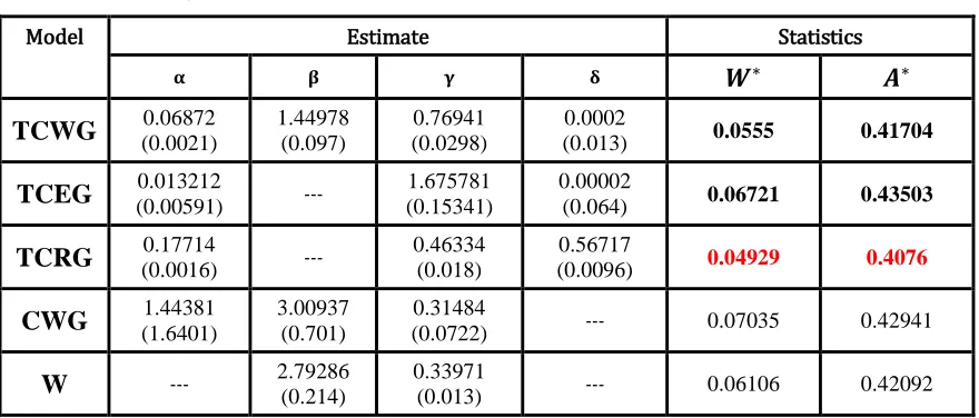
Table 2: MLEs (standard errors in parentheses) for TCWG, TCRG, TCEG, CWG, and W models and the statistics 𝐖∗and 𝐀∗ (second data set)

Model Estimate Statistics

𝛂 𝛃 𝛄 𝛅 𝑾∗ 𝑨∗

TCWG _(0.0021) 0.06872 1.44978 _{(0.097) (0.0298)} 0.76941 _(0.013) 0.0002 0.0555 0.41704

TCEG _(0.00591) 0.013212 --- 1.675781

(0.15341)

0.00002

(0.064) 0.06721 0.43503

TCRG _(0.0016) 0.17714 --- 0.46334

(0.018)

0.56717

(0.0096) 0.04929 0.4076

CWG _(1.6401) 1.44381 3.00937 _{(0.701) (0.0722)} 0.31484 --- 0.07035 0.42941

W --- 2.79286

(0.214)

0.33971

(0.013) --- 0.06106 0.42092

Similarly, the results given in Table 2 illustrate that the TCRG, TCWG and TCEG distributions give better fit than the CWG and W distributions and the TCRG has the lowest A∗_{and W}∗ _{values among all the fitted models, so the TCRG is the best model to fit}

this real data set.

8. Conclusions

and quantile functions. The estimation of parameters is approached by the method of maximum likelihood. Finally, we fit the TCWG model to two real data sets to show its flexibility and potentially as a lifetime distribution. The new model has 11 well known and unknown probability distributions as special cases, 3 of them are new models. We hope that this new distribution may attract wider applications in the lifetime literature. Finally according to the results in tables 1, and 2 it is obvisely that the TCEG and TCRG distributions (as two new sub models of our proposed model) have the lowest A∗_{and W}∗

values among all the fitted models, respectively. So they could be chosen as the best models.

Acknowledgements

The authors are grateful to Professor Abd El Hady N. Ebraheim, Professor and Chair of Professorship Promotion Committee, Institute of Statistical Studies and Research, Cairo University for his valuable comments which improved the original version of the paper. The authors gratefully thanks Professor Mead, Department of Statistics and Insurance, Faculty of Commerce Zagazig University, for his useful suggestions and comments which improved the original version of the paper.

References

1. Adamidis, K. and Loukas, S. (1998). A Lifetime Distribution with Decreasing Failure Rate. Statistics and Probability Letters, 39(1), 35-42.

2. Aryal, G. R. and Tsokos C. P. (2011). Transmuted Weibull distribution: A Generalization of the Weibull Probability Distribution. European Journal of Pure and Applied Mathematics, 4(2), 89-102.

3. Ashour, S.K. and Eltehiwy, M.A. (2013a). Transmuted Exponentiated Lomax Distribution. Australian Journal of Basic and Applied Sciences, 7(7), 658-667. 4. Ashour, S.K. and Eltehiwy, M.A. (2013b). Transmuted Exponentiated Modified

Weibull Distribution. International Journal of Basic and Applied Sciences, 2(3), 258-269.

5. Barreto-Souza, W., de Morais, A. L. and Cordeiro, G. M. (2011). The weibull-geometric distribution. Journal of Statistical Computation and Simulation, 81(5), 645-657.

6. Basu, A. and J., K. (1982). Some recent development in competing risks theory. Survival Analysis, Edited by Crowley, J. and johnson, R. A, Hayvard: IMS, 1, 216-229.

7. Chen, G. and Balakrishnan, N. (1995). A general purpose approximate goodness-of-fit test. Journal of Quality Technology, 27, 154–161.

8. Ebraheim, A. N. (2014). Exponentiated Transmuted Weibull Distribution: A Generalization of the Weibull Distribution. International Journal of

Mathematical, Computational, Physical and Quantum Engineering, 8, (6).

10. Khan, M. S., & King, R. (2013). Transmuted Modified Weibull Distribution: A Generalization of the Modified Weibull Probability Distribution. European Journal of Pure and Applied Mathematics, 6(1), 66-88.

11. Louzada, F., Roman, M. and Cancho, V. G. (2011). The complementary exponential geometric distribution: Model, Properties, and a Comparison with its counterpart. Computational Statistics & Data Analysis, 55(8), 2516-2524.

12. Louzada, F., Marchi, V. and Carpenter, J. (2013). The Complementary Exponentiated Exponential GeometricLifetime Distribution. Hindawi Publishing Corporation. Journal of Probability and Statistics, Article ID 502159.

13. Nichols, M. D. and Padgett, W. J. (2006). A bootstrap control chart for Weibull Percentiles. Quality and Reliability Engineering International, 22, 141-151. 14. Rinne, H. (2009). The Weibull Distribution: A Handbook. CRC Press, London. 15. Shaw, W. T. and Buckley, I. R. C. (2007). The alchemy of probability

distributions: beyond Gram-Charlier expansions and a skew-kurtotic-normal distribution from a rank transmutation map. Research report.